Estimating Lower Limb Kinematics using a Lie Group Constrained EKF and a Reduced Wearable IMU Count
This paper presents an algorithm that makes novel use of a Lie group representation of position and orientation alongside a constrained extended Kalman filter (CEKF) to accurately estimate pelvis, thigh, and shank kinematics during walking using only…
Authors: Luke Sy, Nigel H. Lovell, Stephen J. Redmond
Estimating Lo wer Limb Kinematics using a Lie Group Constrained EKF and a Reduced W earable IMU Count Luke Sy 1 , Nigel H. Lov ell 1 , Stephen J. Redmond 1 , 2 Abstract — This paper pr esents an algorithm that makes no vel use of a Lie group repr esentation of position and orientation alongside a constrained extended Kalman filter (CEKF) to accurately estimate pelvis, thigh, and shank kinematics dur - ing walking using only three wearable inertial sensors. The algorithm iterates through the pr ediction update (kinematic equation), measurement update (pelvis height, zer o velocity update, flat-floor assumption, and covariance limiter), and constraint update (formulation of hinged knee joints and ball- and-socket hip joints). The paper also describes a novel Lie group formulation of the assumptions implemented in the said measurement and constraint updates. Evaluation of the algorithm on nine healthy subjects who walked freely within a 4 × 4 m 2 room shows that the knee and hip joint angle root-mean-squar e err ors (RMSEs) in the sagittal plane f or free walking were 10 . 5 ± 2 . 8 ◦ and 9 . 7 ± 3 . 3 ◦ , respecti vely , while the correlation coefficients (CCs) were 0 . 89 ± 0 . 06 and 0 . 78 ± 0 . 09 , respectively . The evaluation demonstrates a promis- ing application of Lie gr oup representation to inertial motion capture under reduced-sensor -count configuration, impr oving the estimates (i.e., joint angle RMSEs and CCs) for dynamic motion, and enabling better con vergence for our non-linear biomechanical constraints. T o further improve performance, additional information relating the pelvis and ankle kinematics is needed. I . I N T RO D UC T I O N Human pose estimation in volv es tracking the pose (i.e., position and orientation) of body segments from which joint angles can be calculated. It finds application in robotics, virtual reality , animation, and healthcare (e.g., gait analysis). T raditionally , human pose is captured within a laboratory setting using optical motion capture (OMC) systems which can estimate position with up to millimeter accuracy , if well- configured and calibrated. Howe ver , recent miniaturization of inertial measurements units (IMUs) has pav ed the path tow ard inertial motion capture (IMC) systems suitable for prolonged use outside of the laboratory . Commercial IMCs attach one sensor per body segment (OSPS) [1], which may be considered too cumbersome and expensi ve for routine daily use by a consumer due to the number of IMUs required. Each IMU typically tracks the orientation of the attached body segment using an orientation estimation algorithm (e.g., [2, 3]), which is then connected via linked kinematic chain, usually rooted at the pelvis. A reduced-sensor-count (RSC) configuration, where IMUs are placed on a subset of body segments, can improve 1 L. W . Sy , N. H. Lovell, and S. J. Redmond are with the Graduate School of Biomedical Engineering, UNSW Sydney , Australia { l.sy , n.lovell, s.redmond}@unsw .edu.au 2 S. J. Redmond is with the UCD School of Electrical and Electronic Engineering, University College Dublin, stephen.redmond @ucd.ie user comfort while also reducing setup time and system cost. Howe ver , utilizing fewer sensors inherently reduces the amount of kinematic information av ailable; this information must be inferred by enforcing mechanical joint constraints or making dynamic balance assumptions. Developing a com- fortable IMC for routine daily use may facilitate interactive rehabilitation [4, 5], and possibly the study of movement disorder progression to enable predicti ve diagnostics. RSC performance depends on how the algorithm (i) tracks the body pose, and (ii) infers the kinematic information of these body segments lacking attached sensors. The algorithm may leverage our kno wledge of human mo vement either through data obtained in the past (i.e., observed correla- tions between co-movement of different body segments) or by using a simplified model of the human body . Data- driv en approaches (e.g., nearest-neighbor search [6] and bi- directional recurrent neural network [7]) are able to recreate realistic motion suitable for animation-related applications. Howe ver , these approaches are expected to hav e a bias tow ard motions already contained in the database, inherently limiting their use in monitoring pathological gait. Model- based approaches reconstruct body motion using kinematic and biomechanical models (e.g., constrained Kalman filter (KF) [8], extended KF [9], particle filter [10], and windo w- based optimization [11]). W ithin model-based approaches, using optimization-based estimators can be appealing due to its relati ve ease to setup and understand. Howe ver , it can be very inefficient in higher dimensions. When estimating the state across time, a recursiv e estimator can take adv antage of the substructure and reduce the state dimension, making the estimator ef ficient and appropriate for online use [12]. Recent work on pose estimation has sho wn that using a Lie group to represent the states of recursiv e estimator is a promising approach. Such algorithms typically represent the body pose as a chain of linked segments using matrix Lie groups, specifically the special orthogonal group, S O ( n ) , and special Euclidean group, S E ( n ) , where n = 2 , 3 , are the spatial dimensions of the problem. T raditionally , body poses hav e been represented using Euler angles or quaternions [9, 10]. Some early work in the field ([13] and [14]) in vestigated representations and propagation of pose uncertainty , the former in the conte xt of manipulator kinematics and the latter focused on S E (3) . This was followed by the formulation of Lie group-based recursive estimators (e.g., extended KF (EKF) [15] and unscented KF (UKF) [16]). Recently , Lie group based recursiv e estimators were used to solve the pose estimation problem. Cesic et al . estimated pose from marker measurements and achieved significant improvements compared to an Euler angle representation [17]; and even supplemented the approach with an observ ability analysis [18]. Joukov et al . represented pose using S O ( n ) with measurements from IMUs under an OSPS configuration. Results also improved, because the Lie group representation is singularity free [19]. This paper describes a nov el human pose estimator that uses a Lie group representation, propagated iterativ ely using a CEKF to estimate lower body kinematics for an RSC configuration of IMUs. It builds on prior work [8] but instead represents the state v ariables as Lie groups, specif- ically S E (3) , to track both position and orientation ([8] only tracks position). Furthermore, this paper describes a nov el Lie group formulation for assumptions specific to pose estimation, such as zero v elocity update, and biomechanical constraints (e.g., constant thigh length and a hinged knee joint). Note that this algorithm is dif ferent from [19] in that the state (i.e., body pose) was represented as S E (3) instead of S O ( n ) . This representation allo ws for tracking of the global position of the body , incorporating IMU measure- ments in the prediction step, and a simpler implementation of measurement assumptions at the cost of requiring an additional constraint step. The design was motiv ated by the need for a better state variable representation which would potentially better model the biomechanical system to infer the missing kinematic information from uninstrumented body segments. Advancing such algorithms can lead to the dev elopment of a gait assessment tool using as fe w sensors as possible, er gonomically-placed for comfort, to facilitate long-term monitoring of lower body mo vement. I I . A L G O R I T H M D E S C R I P T I O N The proposed algorithm, LGKF-3IMU , uses a similar model and assumptions to our prior work in [8], denoted as CKF-3IMU , albeit expressed in Lie group representation, to estimate the orientation of the pelvis, thighs, and shanks with respect the world frame, W , using only three IMUs attached at the sacrum and shanks, just abov e the ankles (Fig. 1). Using a Lie group representation enables the tracking of not just position but also of orientation singularity free (note that CKF-3IMU only tracked position and assumed orienta- tion as perfect), whilst improving performance for dynamic mov ements and utilizing fewer assumptions. Fig. 2 shows an ov erview of the proposed algorithm. LGKF-3IMU predicts the shank and pelvis positions through double integration of their linear 3D acceleration as measured by the attached IMUs (after a pre-processing step that resolves these accel- erations in the w orld frame). Orientation is obtained from a third party orientation estimation algorithm. T o mitigate positional drift due to sensor noise that accumulates in the double integration of acceleration, the following assumptions are enforced: (1) the ankle 3D velocity and height above the floor are zeroed whenever a footstep is detected; (2) the pelvis Z position is approximated as the length of the unbent leg(s) above the floor . Furthermore, to control the otherwise ev er-gro wing error co variance for the pelvis and ankle positions, a pseudo-measurement equal to the current pose state estimate with a fixed co variance is made. Lastly , biomechanical constraints enforce constant body segment length; ball-and-sockets hip joints; and a hinge knee joint (one degree of freedom (DOF)) with limited range of motion (R OM). The pre- and post-processing parts remains exactly the same as the CKF-3IMU algorithm. Fig. 1. Physical model of the lo wer body used by the algorithm. The circles denote joint positions, the solid lines denote instrumented body segments, whilst the dashed lines denote se gments without IMUs attached (i.e., thighs). Fig. 2. Algorithm overvie w which consists of pre-processing, CEKF , and post-processing. Pre-processing calculates the body segment orientation, inertial body acceleration, and step detection from raw acceleration, a k , angular velocity , ω k , and magnetic north heading, h k , measured by the IMU. The CEKF-based state estimation consists of a prediction (kinematic equation), measurement (orientation, pelvis height, cov ariance limiter, in- termittent zero-velocity update, and flat-floor assumption), and constraint update (thigh length, hinge knee joint, and knee range of motion). Post- processing calculates the left and right thigh orientations, R lt and R rt . A. Lie gr oup and Lie algebra The matrix Lie group G is a group of n × n matrices that is also a smooth manifold (e.g., S E (3) ). Group composition and inv ersion (i.e., matrix multiplication and in version) are smooth operations. Lie algebra g represents a tangent space of a group at the identity element [20]. The ele gance of Lie theory lies in it being able to represent curved objects using a vector space (e.g., Lie group G represented by g ) [21]. The matrix exponential exp G : g → G and matrix loga- rithm log G : G → g establish a local diffeomorphism between the Lie group G and its Lie algebra g . The Lie algebra g is a n × n matrix that can be represented compactly with an n dimensional v ector space. A linear isomorphism between g and R n is gi ven by [ ] ∨ G : g → R n and [ ] ∧ G : R n → g . An illustration of the said mappings are giv en in Fig. 3. Furthermore, the adjoint operators of a Lie group, denoted Lie group G Lie algebra g R n log G exp G [ ] ∨ G [ ] ∧ G Fig. 3. Mapping between Lie group G , Lie algebra g , and a n -dimensional vector space. as Ad G ( X ) , and Lie algebra, denoted as ad G ( X ) will be used in later sections. For a more detailed introduction to Lie groups refer to [12, 21, 22]. B. System, measur ement, and constraint models The system and measurement models are presented below X k = f ( X k - 1 , n k - 1 ) = X k - 1 exp G ([Ω( X k - 1 )+ n k - 1 ] ∧ G ) (1) Z k = h ( X k ) exp G [ m k ] ∧ G , D k = c ( X k ) (2) where k is the time step; X k ∈ G is the system state, an el- ement of state Lie group G ; Ω ( X k ) : G → R p is a non-linear function; n k is a zero-mean process noise vector with cov ari- ance matrix Q k (i.e., n k ∼ N R p ( 0 p × 1 , Q k ) ); Z k ∈ G 1 is the system measurement, an element of measurement Lie group G 1 ; h ( X k ) : G → G 1 is the measurement function; m k is a zero-mean measurement noise vector with cov ariance matrix R k (i.e., m k ∼ N R q ( 0 q × 1 , R k ) ); D k ∈ G 2 is the constraint state, an element of constraint Lie group G 2 ; c ( X k ) : G → G 2 is the equality constraint function the state X k must satisfy . Similar to [17, 23], the state distribution of X k is assumed to be a concentrated Gaussian distribution on Lie groups (i.e., X k = µ k exp G [ ] ∧ G where µ k is the mean of X k and Lie algebra error ∼ N R p ( 0 p × 1 , P ) ) [13]. The Lie group state variables X k model the position, orientation, and velocity of the three instrumented body segments (i.e., pelvis and shanks) as X k = diag T p , T ls , T rs , ˚ v p , ˚ v ls , ˚ v rs ∈ G = S E (3) 3 × R 9 where A T B ∈ S E (3) denotes the pose of body segment B relative to frame A , and ˚ v x = h I 3 × 3 v x 0 1 × 3 1 i is the trivial mapping of a 3D vector to an element in S E (3) . If frame A is not specified, assume reference to the world frame, W . [ ] ∨ , exp [ ] ∧ G , [log ( )] ∨ G , and Ad ( X k ) are con- structed similarly . See [12] for S E (3) operator definitions. C. Lie gr oup constrained EKF (LG-CEKF) The a priori (predicted), a posteriori (updated using measurements), and constrained state (satisfying the state constraint equation, i.e., biomechanical constraints) for time step k are denoted by ˆ µ − k , ˆ µ + k , and ˜ µ + k , respectiv ely . The KF state error a priori and a posteriori cov ariance matrices are denoted as P − k and P + k , respectively . The KF is based on the Lie group EKF , as defined in [23]. 1) Prediction step: estimates the a priori state ˆ µ − k at the next time step and may not necessarily respect the kinematic constraints of the body , so joints may become dislocated after this prediction step. The mean propagation of the three instrumented body segments is governed by Eq. (3) where ˜ Ω + k = Ω( ˜ µ + k ) and Ω( X k ) is the motion model for the three instrumented body segments. For the sake of brevity , only the motion model of the position, orientation, and velocity for body segment b is sho wn (Eqs. (4)). The measured acceleration and orientation of segment B are denoted as ˘ a B k and ˘ R B k . The process noise for body segment b is shown in Eq. (5) where σ b acc and σ b q ori denote the noise variances of the measured acceleration and orientation. Note that one may use the measured angular v elocity to predict orientation. Ho wev er , we chose setting angular velocity to zero to simplify computations related to position, knowing that the orientation will be updated in the measurement step using measurements from a third party orientation estimation algorithm, accounting for angular velocity . ˆ µ − k +1 = ˜ µ + k exp G ([ ˜ Ω + k ] ∧ G ) (3) Ω b ( X k ) = [(∆ t v b k + ∆ t 2 2 ˘ a b k ) T ˘ R b k 0 1 × 3 ∆ t ( ˘ a b k ) T ] T (4) n b = [ ∆ t 2 2 ( σ b acc ) T ( σ b q ori ) T ∆ t ( σ b acc ) T ] T (5) The state error covariance matrix propagation is governed by Eq. (6) where F k represents the matrix Lie group equiv- alent to the Jacobian of f ( X k - 1 , n k - 1 ) , C k represents the linearization of the motion model, Q k is constructed from with diagonal v alues from n b , and µ k = µ k exp G ([ ] ∧ G ) represents the state with infinitesimal perturbation . Refer to the supplementary material [24] for the explicit definition of the motion model, Ω k ( X k ) , and C k . P − k +1 = F k P + k F T k + Φ G ( ˆ Ω k ) Q k Φ G ( ˆ Ω k ) T (6) F k = Ad G (exp G ( − [ ˆ Ω k ] ∧ G )) + Φ G ( ˆ Ω k ) C k (7) C k = ∂ ∂ Ω ( µ k ) | =0 , (8) Φ G ( X k ) = P ∞ i =0 ( − 1) i ( i +1)! ad G ( X k ) i (9) 2) Measurement update: estimates the state at the next time step by: (i) updating the orientation state using new orientation measurements of body segments; (ii) encouraging pelvis Z position to be close to initial standing height z p , and by; (iii) encouraging ankle velocity to approach zero, and the ankle Z position to be close to the floor lev el, z f . The a posteriori state ˆ µ + k is calculated following the Lie EKF equations belo w . H k can be seen as the matrix Lie group equiv alent to the Jacobian of h ( X k ) ; and is defined as the concatenation of H ori and H mp . H ls and/or H rs are also concatenated to H k when the left and/or right foot contact is detected (See [8, Eq. (9)]). Each component matrix will be described later . Z k , h ( X k ) , and R k are constructed similarly to H k but combined using diag instead of concatenation (e.g., R k = diag ( σ ori , σ mp ) ) K k = P − k H T k ( H k P − k H T k + R k ) − 1 (10) ν k = K k ([log G 1 h ( ˆ µ − k ) − 1 Z k ] ∨ G 1 ) (11) ˆ µ + k = ˆ µ − k exp G ([ ν k ] ∧ G ) (12) H k = ∂ ∂ [log G 1 h ( ˆ µ − k ) − 1 h ( µ k ) ] ∨ G 1 | =0 (13) The measurement functions of the (i) orientation update, (ii) pelvis height assumption, and (iii) ankle velocity and flat floor assumptions are defined by Eqs. (14)-(17) with measurement noise variances σ 2 ori ( 9 × 1 vector), σ 2 mp ( 1 × 1 vector), and σ 2 ls ( 4 × 1 vector), respectiv ely . I i × j and 0 i × j denote i × j identity and zero matrices; i x , i y , i z , and i 0 denote 4 × 1 vectors whose 1 st to 4 th row , respecti vely , are 1 , while the rest are 0 ; and the operator is as defined in [12, Eq. (72)]. H ori , H mp , and H ls (Eqs. (18)-(20)) are calculated by applying Eq. (13) to their corresponding measurement function, follo wed by tedious algebraic manipulation and first order linearization (i.e., exp([ ] ∧ ) ≈ I + [ ] ∧ ). See details in the supplementary material [24]. h ori ( X k ) = diag ( R p k , R ls k , R rs k ) (14) Z ori = diag ( ˘ R p k , ˘ R ls k , ˘ R rs k ) (15) h mp ( X k ) = i T z T p i 0 , Z mp = z p (16) h ls ( X k ) = v ls i T z T ls i 0 , Z ls = 0 3 × 1 z f (17) H ori = 0 3 × 3 I 3 × 3 0 3 × 3 I 3 × 3 0 9 × 9 0 3 × 3 I 3 × 3 (18) H mp = i T z ¯ T p [ i 0 ] 0 1 × 6 0 1 × 6 0 1 × 9 (19) H ls = . . . pos. ori. col. . . . I 3 × 3 | {z } . . . z }| { i T z ¯ T ls [ i 0 ] vel. col. (20) Lastly , the co variance limiter pre vents the cov ariance from growing indefinitely and from becoming badly conditioned, as will happen naturally when tracking the global position of the pelvis and ankles without any global position reference. At this step, a pseudo-measurement equal to the current state ˆ µ + k is used (implemented by H lim = I 18 × 18 0 18 × 9 ) with some measurement noise of v ariance σ lim ( 9 × 1 v ector). The cov ariance P + k is then calculated through Eqs. (21)-(23). H 0 k = H T k H T lim T , R 0 k = diag ([ σ k σ lim ]) (21) K 0 k = P − k H 0 T k H 0 k P − k H 0 T k + R 0 − 1 (22) P + k = Φ G ( ν k ) ( I − K 0 k H 0 k ) P − k Φ G ( ν k ) T (23) 3) Satisfying biomechanical constraints: After the pre- diction and measurement updates, above, the body joints may have become dislocated, or joint angles extend beyond their allowed range. This update corrects the kinematic state estimates to satisfy the biomechanical constraints of the human body by projecting the current a posteriori state ˆ µ + k estimate onto the constraint surface, guided by our uncertainty in each state variable, encoded by P + k . The constraint equations enforce the follo wing biomechanical limitations: (i) the length of estimated thigh v ectors ( || τ lt || and || τ rt || ) equal the thigh lengths d lt and d rt ; (ii) both knees act as hinge joints (formulation similar to [10, Sec. 2.3 Eqs. (4)]); and (iii) the knee joint angle is confined to realistic ROM. The constrained state ˜ µ + k can be calculated using the equations belo w , similar to the measurement update of [23] with zero noise where C k = C T L,k C T R,k T . C L,k is the concatenation of C ltl,k , C lkh,k , and C lkr,k ; the last matrix is not concatenated when the knee angle, α lk , is bounded (i.e., α lk,min ≤ α lk ≤ α lk,max ). Each component matrix will be described later . C R,k can be deri ved similarly , while D k and c ( X k ) are constructed similarly to Z k . K k = P + k C T k ( C k P + k C T k ) − 1 (24) ν k = K k ([log G 2 ( c ( ˆ µ + k ) − 1 D k )] ∨ G 2 ) (25) ˜ µ + k = ˆ µ + k exp G [ ν k ] ∧ G (26) C k = ∂ ∂ [log G 2 c ˆ µ + k − 1 c ( µ k ) ] ∨ G 2 | =0 (27) The constraint functions are similar to [8, Sec. II-E.3] but expressed under S E (3) state variables. Firstly , the thigh length constraint is shown in Eq. (30) where τ lt z ( ˜ µ + k ) denotes the thigh vector . Secondly , the hinge knee joint constraint is defined by Eq. (31). Thirdly , the knee ROM constraint is defined by Eq. (34) and is only enforced if the knee angle, α lk , is outside the allowed R OM. The bounded knee angle, α 0 lk , is calculated by Eqs. (32) and (33). Lastly . C ltl,k , C lkh,k , and C lkr,k are calculated by applying Eq. (27) to their corresponding constraint functions, similar to H mp . Refer to the supplementary material for full deriv ation [24]. p p lh = 0 d p 2 0 1 T , ls p lk = 0 0 d ls 1 T (28) τ lt z ( ˜ µ + k ) = E z }| { I 3 × 3 0 3 × 1 hip joint pos. z }| { T p p p lh − knee joint pos. z }| { T ls ls p lk (29) c ltl ( ˜ µ + k ) = τ lt z ( ˜ µ + k ) T τ lt z ( ˜ µ + k ) − ( d lt ) 2 = 0 = D ltl (30) c lkh ( ˜ µ + k ) = ( r ls y ) T τ lt z = 0 = D lkh (31) α 0 lk = min ( α lk,max , max ( α lk,min , α lk )) (32) α lk = tan − 1 − ( r ls z ) T r lt z − ( r ls x ) T r lt z + π 2 (33) c lkr ( ˜ µ + k ) = (( r ls z ) T cos( α 0 lk – π 2 ) – ( r ls x ) T sin( α 0 lk – π 2 )) r lt z = 0 = D lkr (34) I I I . E X P E R I M E N T The dataset from [8] was used to ev aluate LGKF-3IMU . It inv olved movements listed in T able I from nine healthy subjects ( 7 men and 2 women, weight 63 . 0 ± 6 . 8 kg, height 1 . 70 ± 0 . 06 m, age 24 . 6 ± 3 . 9 years old), with no known gait abnormalities. Raw data were captured using a commercial IMC (i.e., Xsens A winda) compared against a benchmark OMC (i.e., V icon) within an ~ 4 × 4 m 2 capture area. T ABLE I T Y P E S O F M OV E M E N T S D O N E I N T H E V A L I D A T I O N E X P E R I M E N T Movement Description Duration Group W alk W alk straight and return ∼ 30 s F Figure-of-eight W alk along figure-of-eight path ∼ 60 s F Zig-zag W alk along zig-zag path ∼ 60 s F 5-minute walk Unscripted walk and stand ∼ 300 s F Speedskater Speedskater on the spot ∼ 30 s D Jog Jog straight and return ∼ 30 s D Jumping jacks Jumping jacks on the spot ∼ 30 s D High knee jog High knee jog on the spot ∼ 30 s D F denotes free walk, D denotes dynamic Unless stated, calibration and system parameters similar to [8] were assumed. The algorithm and calculations were implemented using Matlab 2018b . The initial position, ori- entation, and velocity ( ˜ µ + 0 ) were obtained from the V icon benchmark system. P + 0 was set to 0 . 5 I 27 × 27 . The variance parameters used to generate the process and measurement error covariance matrix Q and R are shown in T able II. T ABLE II V A R I A N C E PA R A M E T E R S F O R G E N E R A T I N G T H E P R O C E S S A N D M E A S U R E M E N T E R RO R C O V A R I A N C E M ATR I C E S , Q A N D R . Q Parameters R Parameters σ 2 acc σ 2 qor i σ 2 ori σ 2 mp σ 2 ls and σ 2 rs σ 2 lim (m 2 .s − 4 ) (m 2 ) (m 2 .s − 2 and m 2 ) (m 2 ) 10 2 1 9 10 3 1 12 10 − 2 0 . 1 [0 . 01 1 3 10 − 4 ] 10 1 18 where 1 n is an 1 × n row vector with all elements equal to 1 . Lastly , the ev aluation was done using the following met- rics: (1) joint angles RMSE with bias remo ved and coefficient of correlation (CC) of the hip in the Y , X, and Z planes and of the knee in the Y plane; and (2) T otal trav elled distance (TTD) deviation (i.e., TTD error with respect to the actual TTD) of the ankles. Refer to [8, Sec. III] for more details. I V . R E S U LT S Fig. 4 shows the knee and hip joint angle RMSE (bias remov ed) and CC compared against the OMC output. Y , X, and Z refers to the sagittal, frontal, and transv erse planes, respectiv ely . Fig. 5 sho ws a sample W alk trial. T able III shows the TTD deviation at the ankles for free walk and jogging. Refer to http://bit.ly/3bHlVG9 for video reconstructions of sample trials. Fig. 4. The CC of knee (Y) and hip (Y , X, Z) joint angles for LGKF-3IMU (prefix LG ) and CKF-3IMU (prefix C ) at each motion type. Fig. 5. Knee (Y) and hip (Y , X, Z) joint angle output of LGKF-3IMU in comparison with the benchmark system (V icon) for a W alk trial. The subject walked straight from t = 0 to 3 s, turned 180 ◦ around from t = 3 to 5 . 5 s, and walk ed straight to the original starting point from 5 . 5 s until the end. V . D I S C U S S I O N Fig. 4 sho ws that although there was minimal hip and knee joint angle RMSE and CC improv ement for free walk T ABLE III T OTAL T R A V E L L E D D I S TA N C E ( T T D ) D E V I AT I O N F RO M O P T I C A L M OT I O N C A P T U R E ( O M C ) S Y S T E M AT T H E A N K L E S CKF-3IMU LGKF-3IMU Left Right Left Right Free walk 3.81% 3.61% 8.13% 8.13% Jog 24.05% 28.16% 18.58% 21.54% between CKF-3IMU and LGKF-3IMU , there was significant improv ement for most dynamic mov ements, specifically , speedskater , jog, and high knee jog, indicating that the Lie group representation has indeed made the pose estimator capable of tracking more ADLs and not just walking. This result also agrees with [19]. Similar to IMC based systems, LGKF-3IMU also follo ws the trend of having sagittal (Y axis) joint angles similar to that captured by OMC systems ( 0 . 89 knee Y and 0 . 78 hip Y CCs), b ut with significant difference in frontal and transverse (X and Z axis) joint angles [8, 25]. Similar qualitativ e observations can be seen in Fig. 5, specifically , there were larger angle change for hip X ( t = 0 to 3 s and t = 6 to 8 s) and hip Z ( t = 3 to 5 s). The knee and hip joint angle RMSEs and CCs of CKF- 3IMU , LGKF-3IMU , OSPS and related literature for free walking are shown in T able IV [8, 25]. Although the biased joint angle RMSE for LGKF-3IMU is comparable with OSPS and Cloete’ s ( < 6 ◦ ), the unbiased results show that utilizing fewer sensors does reduce accuracy somewhat [25]. Despite LGKF-3IMU achieving good joint angle CCs in the sagittal plane, the unbiased joint angle RMSE ( > 5 ◦ ) makes its utility in clinical applications uncertain [26]. Furthermore, LGKF-3IMU shares the limitations of CKF-3IMU during longer-term tracking of ADL, being unable to handle the activities of sitting, lying down, or climbing stairs due to the pelvis height and/or flat floor assumptions; and unable to track people with v arus or valgus deformity , or those capable of hyperextending the knee due to the algorithm’ s hinge knee joint and R OM constraints. Dev eloping solutions to further increase accuracy and overcome the said limitations (e.g., measuring inter -sensor distance, incorporating dynamics in addition to kinematics, or lev eraging long-term recordings and gait patterns) will be part of future work. Comparing processing times, LG-CEKF was slower than CKF but can still be used in real time; specifically , LG-CEKF and CKF processed a 1,000-frame sequence in ~ 2 and ~ 0 . 7 seconds, respectiv ely , on an Intel Core i5-6500 3.2 GHz CPU [8], while the algorithm in [11] took 7.5 minutes on a quad- core Intel Core i7 3.5 GHz CPU. All set-ups used single-core non-optimized Matlab code. T able III shows that despite successful reconstruction of relativ e pose, LGKF-3IMU had worse TTD for free walking than CKF-3IMU . It can be observed from the sample video trial that the LGKF-3IMU had less displacement during the turn around (i.e., high rotational change). LGKF-3IMU was able to achieve comparable and occa- sionally better results than CKF-3IMU using fewer assump- tions (i.e., encourage pelvis x and y position to approach the av erage of the left and right ankle x and y positions T ABLE IV K N E E A N D H I P A N G L E R M S E ( T O P ) A N D C C ( B OT T O M ) O F CKF-3IMU , OSPS , A N D R E L A T E D L I T E R A T U R E Joint Angle RMSE ( ◦ ) knee sagittal hip sagittal hip frontal hip transverse CKF- 3IMU biased 11 . 1 ± 2 . 9 11 . 8 ± 3 . 2 7 . 5 ± 3 . 1 17 . 5 ± 4 . 7 mean − 1 . 2 ± 4 . 2 − 4 . 3 ± 4 . 4 − 2 . 2 ± 4 . 2 − 4 . 0 ± 9 . 7 no bias 10 . 0 ± 2 . 8 9 . 9 ± 3 . 1 6 . 1 ± 1 . 8 13 . 9 ± 2 . 4 LGKF- 3IMU biased 13 . 9 ± 4 . 5 11 . 6 ± 4 . 1 8 . 9 ± 4 . 2 17 . 0 ± 4 . 4 mean 8 . 1 ± 4 . 8 4 . 6 ± 4 . 3 − 4 . 0 ± 5 . 3 − 3 . 3 ± 9 . 0 no bias 10 . 5 ± 2 . 8 9 . 7 ± 3 . 3 6 . 4 ± 2 . 1 13 . 7 ± 2 . 4 OSPS biased 7 . 9 ± 3 . 2 12 . 4 ± 6 . 0 6 . 2 ± 2 . 6 19 . 8 ± 6 . 6 mean 0 . 2 ± 6 . 1 − 10 . 9 ± 7 . 4 0 . 2 ± 2 . 5 8 . 8 ± 8 . 8 no bias 5 . 0 ± 1 . 7 3 . 6 ± 1 . 7 4 . 1 ± 2 . 2 11 . 9 ± 4 . 3 Cloete et al .[25] biased 11 . 5 ± 6 . 4 16 . 9 ± 3 . 6 9 . 6 ± 5 . 1 16 . 0 ± 8 . 8 no bias 8 . 5 ± 5 . 0 5 . 8 ± 3 . 8 7 . 3 ± 5 . 2 7 . 9 ± 4 . 9 Joint Angle CC knee sagittal hip sagittal hip frontal hip transverse CKF-3IMU 0 . 87 ± 0 . 08 0 . 74 ± 0 . 11 0 . 64 ± 0 . 12 0 . 33 ± 0 . 12 LGKF-3IMU 0 . 89 ± 0 . 06 0 . 78 ± 0 . 09 0 . 63 ± 0 . 12 0 . 38 ± 0 . 12 OSPS 0 . 97 ± 0 . 03 0 . 95 ± 0 . 06 0 . 72 ± 0 . 19 0 . 26 ± 0 . 20 Cloete et al .[25] 0 . 89 ± 0 . 15 0 . 94 ± 0 . 08 0 . 55 ± 0 . 40 0 . 54 ± 0 . 20 during the measurement update, and the pre vention of knee angle decrease during the constraint update [8, Sec. II-E.2 and 3]); and only at one iteration ( CKF-3IMU used an iterativ e projection scheme called smoothly constrained KF), indicating the robustness brought by the Lie group represen- tation. Furthermore, LGKF-3IMU does not assume perfect orientation during the constraint update, in contrast to CKF- 3IMU , which can be beneficial if new sensor information that informs segment orientation is added. V I . C O N C L U S I O N This paper presented a Lie group CEKF-based algorithm ( LGKF-3IMU ) to estimate lower limb kinematics using a reduced sensor count configuration, and without using any reference motion database. The knee and hip joint angle RM- SEs in the sagittal plane for free walking were 10 . 5 ± 2 . 8 ◦ and 9 . 7 ± 3 . 3 ◦ , respectiv ely , while the CCs were 0 . 89 ± 0 . 06 and 0 . 78 ± 0 . 09 , respectively . W e also showed that LGKF-3IMU improv es estimates for dynamic motion, and enables better con ver gence for our non-linear biomechanical constraints. T o further improv e performance, additional information relating the pelvis and ankle kinematics is needed (e.g., utilize sen- sors that gi ve pelvis distance or position relative to the ankle). The source code for the LG-CEKF algorithm, supplementary material, and links to sample videos will be made av ailable at https://git.io/Jv3oF . A C K N OW L E D G E M E N T This research was supported by an Australian Government Research Training Program (R TP) Scholarship. R E F E R E N C E S [1] D. Roetenberg, H. Luinge, and P . Slycke, “Xsens MVN: Full 6DOF human motion tracking using miniature inertial sensors, ” Xsens Motion T echnol. BV , T ech. Rep , vol. 1, 2009. [2] M. B. Del Rosario, N. H. Lovell, and S. J. Redmond, “Quaternion- based complementary filter for attitude determination of a smart- phone, ” IEEE Sens. J. , vol. 16, no. 15, pp. 6008–6017, 2016. [3] M. B. Del Rosario, P . Ngo, H. Khamis, N. H. Lo vell, S. J. Redmond, P . Ngo, N. H. Lov ell, and S. J. Redmond, “Computationally ef ficient adaptiv e error-state Kalman filter for attitude estimation, ” IEEE Sens. J. , vol. 18, no. 22, pp. 9332–9342, 2018. [4] R. Lloréns, J. A. Gil-Gómez, M. Alcañiz, C. Colomer, and E. Noé, “Improvement in balance using a virtual reality-based stepping exercise: A randomized controlled trial inv olving individuals with chronic stroke, ” Clin. Rehabil. , vol. 29, no. 3, pp. 261–268, 2015. [5] P . Shull, K. Lurie, M. Shin, T . Besier, and M. Cutkosk y, “Haptic gait retraining for knee osteoarthritis treatment, ” in 2010 IEEE Haptics Symp. , IEEE, 2010, pp. 409–416. [6] J. T autges, A. Zinke, B. Krüger, J. Baumann, A. W eber, T . Helten, M. Müller, H. Seidel, and B. Eberhardt, “Motion reconstruction using sparse accelerometer data, ” ACM T rans. Graph. , v ol. 30, no. 3, p. 18, 2011. eprint: 1006.4903 . [7] Y . Huang, M. Kaufmann, E. Aksan, M. J. Black, O. Hilliges, and G. Pons-Moll, “Deep inertial poser: Learning to reconstruct human pose from sparse inertial measurements in real time, ” in SIGGRAPH Asia 2018 T ech. P ap. SIGGRAPH Asia 2018 , Association for Computing Machinery , Inc, 2018. eprint: 1810.04703 . [8] L. Sy, M. Raitor, M. D. Rosario, H. Khamis, L. Kark, N. H. Lovell, and S. J. Redmond, “Estimating Lo wer Limb Kinematics using a Reduced W earable Sensor Count, ” 2020. T o be published. [9] J. F . Lin and D. Kuli ´ c, “Human pose recovery using wireless inertial measurement units, ” Physiol. Meas. , vol. 33, no. 12, pp. 2099–2115, 2012. [10] X. L. Meng, Z. Q. Zhang, S. Y . Sun, J. K. Wu, and W . C. W ong, “Biomechanical model-based displacement estimation in micro-sensor motion capture, ” Meas. Sci. T echnol. , v ol. 23, no. 5, p. 055 101, 2012. [11] T . von Marcard, B. Rosenhahn, M. J. Black, and G. Pons-Moll, “Sparse inertial poser: Automatic 3D human pose estimation from sparse IMUs, ” in Comput. Graph. F orum , W iley Online Library , vol. 36, 2017, pp. 349–360. eprint: 1703.08014 . [12] T . D. Barfoot, State Estimation for Robotics . Cambridge University Press, 2017. [13] Y . W ang and G. S. Chirikjian, “Error propagation on the Euclidean group with applications to manipulator kinematics, ” IEEE T rans. Robot. , vol. 22, no. 4, pp. 591–602, 2006. [14] T . D. Barfoot and P . T . Furgale, “Associating uncertainty with three- dimensional poses for use in estimation problems, ” IEEE T rans. Robot. , vol. 30, no. 3, pp. 679–693, 2014. [15] G. Bourmaud, R. Mégret, M. Arnaudon, and A. Giremus, “Continuous-Discrete Extended Kalman Filter on Matrix Lie Groups Using Concentrated Gaussian Distributions, ” J. Math. Imaging V is. , vol. 51, no. 1, pp. 209–228, 2014. [16] M. Brossard, S. Bonnabel, and J. P . Condomines, “Unscented Kalman filtering on Lie groups, ” in IEEE Int. Conf. Intell. Robot. Syst. , vol. 2017-Septe, 2017, pp. 2485–2491. [17] J. ´ Cesi ´ c, V . Jouko v, I. Petro vi ´ c, and D. Kuli ´ c, “Full body human motion estimation on lie groups using 3D marker position measure- ments, ” IEEE-RAS Int. Conf. Humanoid Robot. , pp. 826–833, 2016. [18] V . Jouko v, J. Cesic, K. W estermann, I. Marko vic, I. Petrovic, and D. Kulic, “Estimation and Observability Analysis of Human Motion on Lie Groups, ” IEEE T rans. Cybern. , pp. 1–12, 2019. [19] V . Joukov, J. Cesic, K. W estermann, I. Markovic, D. Kulic, and I. Petrovic, “Human motion estimation on Lie groups using IMU measurements, ” IEEE Int. Conf . Intell. Robot. Syst. , vol. 2017-Septe, pp. 1965–1972, 2017. [20] J. M. Selig, “Lie groups and lie algebras in robotics, ” in Comput. Noncommutative Algebr . Appl. Springer, 2004, pp. 101–125. [21] J. Stillwell, Naive lie theory . Springer Science & Business Media, 2008. [22] G. S. Chirikjian, Stochastic models, information theory , and lie gr oups, volume 2: Analytic methods and modern applications . Springer Science & Business Media, 2011, vol. 2. [23] G. Bourmaud, A. Giremus, Y . Berthoumieu, and G. Bourmaud, “Discrete extended Kalman filter on lie groups, ” pp. 1–5, 2013. [24] L. Sy, N. H. Lovell, and S. J. Redmond, Supplementary material to estimating lower limb kinematics using a lie group constrained ekf and a reduced wearable imu count . [25] T . Cloete and C. Scheffer, “Benchmarking of a full-body inertial motion capture system for clinical gait analysis, ” in 2008 30th Annu. Int. Conf. IEEE Eng. Med. Biol. Soc. , IEEE, 2008, pp. 4579–4582. [26] J. L. McGinley , R. Baker, R. W olfe, and M. E. Morris, “The reliability of three-dimensional kinematic gait measurements: A systematic review , ” Gait P osture , vol. 29, no. 3, pp. 360–369, 2009.
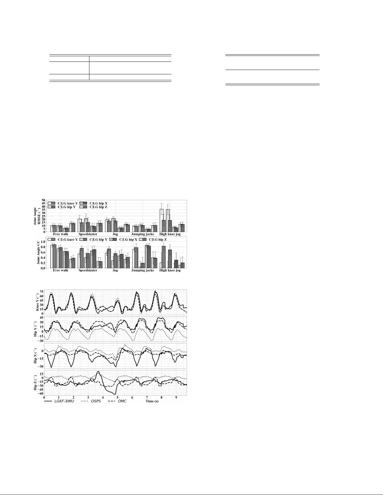
Original Paper
Loading high-quality paper...
Comments & Academic Discussion
Loading comments...
Leave a Comment