Homogeneous Models of Nonlinear Circuits

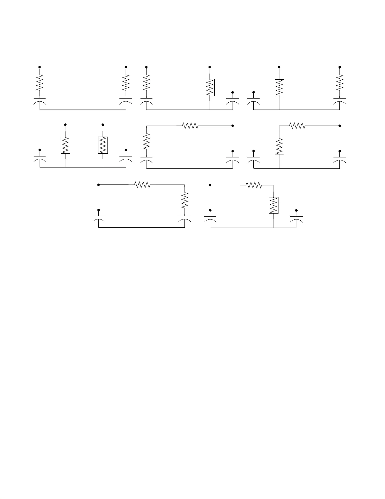
Homogeneous Mo dels of Nonlinear Circuits ∗ Ricardo Riaza † Abstract This pap er dev elops a general approac h to nonlinear circuit mo delling aimed at pre- serving the in trinsic symmetry of electrica l circuits when form ulating reduced mo dels. The goal is to pro vide a framework accommodating su c h red u ctio ns in a global manner and without any loss of generalit y in the working assum ptions; sp eciﬁcally , we av oid global hyp otheses imp osing the existence of a cl assical circuit v ariable cont rolling eac h device. Classical (vol tage/curren t but also ﬂ ux/c harge) mo dels are easily ob tained as particular cases of a general h omog eneous mod el. Our app roac h extends the results in tr odu ced for lin ea r circuits in a previous pap er, b y means of a systematic use of global p arametrizations of smo oth planar curve s. This makes it p ossible to form ulate reduced mo dels in terms of homogeneous v ariables also in the nonlinear cont ext: con- trary t o volt ages and curr en ts (and al so to ﬂuxes and c harges), homogeneous v ariables qualify as stat e v ariables for s mooth, uncoupled circuits without any restriction o n the c haracteristics of devices. The inh eren t symmetry of this formalism mak es it p ossible to ad d ress in b road generalit y certain analytical problems in nonlinear circuit theory , suc h as the sta te-space problem a nd related issues inv olving impasse phenomena. Our framew ork applies also to circuits with memr isto rs, and can b e extended to include con trolled sources and coupling eﬀects. Sev eral examples illustrate the resu lts. Index T erms: Analog circuits, circuit analysis, nonlinear circuits, memristors, diﬀerential- algebraic equations, geometry , netw o rk t heory , nonlinear systems. 1 In tro duction W e extend in this pap er the approach of [25 ] to the nonlinear circuit con text. Our main goal is to introduce and exploit, for analytical purp oses, circuit mo dels of the form A c ψ ′ c ( u c ) u ′ c + A l ψ l ( u l ) + A r ψ r ( u r ) = 0 (1a) B c ζ c ( u c ) + B l ζ ′ l ( u l ) u ′ l + B r ζ r ( u r ) = 0 , (1b) where we use the prime ′ to denote diﬀeren tia tion (with res p ect to time when no a rgumen t is giv en, as e.g. in u ′ c ). This mo del is form ulated in terms of certain ve ctor-v alued homo gen e o us ∗ This is the author ’s ﬁnal version of a paper published in the IEEE T r ansactions on Cir cuits and Syst ems I - R e gular Pap ers , vol. 67, no. 6, June 2 0 20, pp. 2 002-2015 : http://doi .org/10.1109/TCSI.2020.2968306 † Depto. de Matem´ atica Aplicada a las TIC & Information P r ocess ing and T elecommunications Cen ter, ETS Ingenieros de T elecomunicaci´ on, Universidad Polit´ ecnica de Madrid, Spain. ricardo.riaza @upm.es . 1 variables , namely u c , u l and u r for (smo o th, p oss ibly nonlinear) capacitors, inductors and resistors. Indep end en t sources can b e handled join tly with resistors just b y rewriting the maps ψ r and ζ r as ψ r ( u r , t ) and ζ r ( u r , t ), respectiv ely; memristors can also be easily included in the mo del and will b e considered later. T o get a brief o v erview b efore going in to details, the reader may think of the matrices A = ( A c A l A r ) a nd B = ( B c B l B r ) as describing t he circuit top ology (with Kirchh oﬀ la ws reading a s Ai = 0, B v = 0), whereas the so-called p ar ametrization maps ψ c , ζ c , etc. comprise the characteristics o f the circuit devices. Solutions in terms o f classical circuit v ariables (curren t, voltage, c harge and ﬂux) are explicitly o btained from those of (1) by means o f the relations i r = ψ r ( u r ), v r = ζ r ( u r ), σ c = ψ c ( u c ), etc. (cf. subsection 2.4). Note also that mo dels fo rm ulated in terms of classical circuit v ariables are comprised in (1) as particular cases, being obtained in a straigh t forw ard manner by means of sp eciﬁc choice s of the maps ψ c , ζ c , etc.: the idea is that, for example, a v olta ge-con trol assumption for all resistors is captured in the mo del b y setting ζ r = id, so that u r amoun ts to the v ector of bra nc h v o ltages v r and then ψ r describes the v oltage-to- curren t c haracteristics. W e e mphasize t ha t the s cop e of (1) ex tends bey ond these particular (classical) cases, pro viding a truly general and ﬂexible framew ork for nonlinear circuit mo delling and a na lys is. W e refer the reader to Section 2 for further details. A ke y elemen t in o ur approac h is the parametric f o rm of Ohm’s law, whic h reads as i = pu (2a) v = q u. (2b) Here w e are dealing with an individual device (a linear resis tor) so that all v ariables and parameters in (2) are scalar. W e delib erately a void the curren t-controlled form v = z i ( z is either the impedance or the re sistance, depending on the conte xt) and the voltage-con trolled one i = y v , b ecause b oth lac k generality: indeed, the former do es not accommo date an op en- circuit (gov erned b y the relation i = 0), and the latter excludes a short- circuit (fo r whic h v = 0). Ho w ev er, all cases are cov ered in terms of the parameters p and q in (2), whic h are assumed not to v a nis h simultaneous ly and therefore deﬁne homogeneous co ordinates of a pro jectiv e line (cf. [2 5]); under the obvious non-v anishing assump tions, w e get either the imp edance/res istance in the form z = q /p or the admittance/conductance as y = p/q . In (2), u is a n abstract (so-called homo gene ous ) v ariable whic h will qualify as a state v ariable in all p ossible parameter scenarios, by contrast to both i and v , in ligh t of the exclu ded conﬁgurations resulting f rom the aforemen tioned classical forms o f Ohm’s la w. The exte nsion of this ide a to the nonlinear con text pro ceeds through the nonlinear coun- terpart of (2); that is, w e w ould no w des crib e the c haracteristic of a nonlinear resis tor as i = ψ ( u ) (3a) v = ζ ( u ) , (3b) for certain nonlinear functions ψ , ζ and a giv en parameter u . The k ey fact here is that this description is feasible in a global sense for (smo oth and uncoupled) nonlinear devices, as a 2 result of the classiﬁcation theorem for smo oth planar curv es. This w a y w e will describ e the c haracteristic of each individual device, under a smo othness assumption to b e ma de precise later, in terms of a globally deﬁned parameter u , lying either o n the real line R or on the 1- sphere (circle) S 1 ; this parameter brings to the nonlinear context the idea of a homogeneous v aria ble discussed ab o v e. Here w e are assuming that the de vice is a re sistor (in other w ords, that its c haracteristic relates curren t and v oltage), but the same applies in a natural manner to reactiv e devices, whose c haracteristics in volv e either the electrical c harge or the magnetic ﬂux, and also to memristors. These ideas are presen ted in Section 2 where, go ing from the device lev el of the last t wo paragraphs to the circuit le v el, w e deriv e and discuss in detail the model (1). In the abse nce of coupling eﬀects, the v ector-v alued maps ψ c , ζ c , etc. a re gua r a n teed to exist in a g lo bal sense by the classiﬁcation theorem men tioned ab o v e, hav ing a (sa y) diago nal form (that is, the k - th comp onen t of each map depends only o n the k -th comp onen t of its argumen t); note also that coupling eﬀects ma y b e natura lly accommo dated in (1) b y deﬂating this diagonal requiremen t (cf. subsection 2.6). Indep enden t sources can be included just by letting ψ r and ζ r dep end also on t (e.g. for an ideal indep enden t source injecting a curren t i s ( t ) just set ψ ( t ) = i s ( t ) and ζ ( u ) = u ); the extension is straigh tforw ard a nd w e exclude indep enden t sources throug ho ut the do cumen t only for the sake of brevit y . Dependen t sources can b e handled in a similar ma nner to coupled devices, as discussed in subsection 2 .6. Ev en if a detailed discussion can b e found in Section 2, w e summarize here some ad- v antages of our homogeneous a pproac h. Mo dels of the form (1) make it p ossible to get rid of unnecessarily restrictiv e assumptions on controlling v ariables for the diﬀeren t circuit devices, m uc h as in the linear case the homogeneous formalism av oids the need to impose an imp edance (curren t-con trolled) or an admittance (v olta ge-con trolled) des cription f or eac h individual dev ice. And ev en if exp licit descriptions in terms of a classical circuit v ariable (curren t, v olta ge, c ha rge or ﬂux) are used, all suc h descriptions can b e accommo dated in (1), whic h this w a y deﬁnes a broadly general theoretical fra mew ork for nonlinear circuit mo delling. Note that the ho mo g ene ous setting also allo ws o ne to handle, in a glo bal man- ner, reduced mo dels in situations in whic h certain devices do not admit a g lobal explicit description in terms of a classical circuit v ar ia ble: an example o f this, in volving a h ysteresis lo op, can b e found in subsection 2.5 . In Section 3 we apply the ho mog ene ous f r a mew ork to address certain analytical problems in nonlinear circuit theory , inv o lving the state-space problem a nd a lso t he structure of the so-called regular and impasse se ts. W e extend in less detail the results to the memristiv e con text in Section 4. Finally , concluding remarks can b e found in Section 5. 2 Homogeneous mo delling 2.1 Linear circ uit s The homogeneous formalism in the linear setting is dev elop ed in [25], and naturally drives parametric analyses of linear circuits to t he con text o f pr o jectiv e geometry (re lated ideas can 3 b e found in [3, 4, 2 0 , 28], although none of these w o rks extend the results to t he nonlinear con text). This fr a mew ork leads to a completely general reduction of linear circuits, without an y restriction on the con trolling v ariables of individual devices, and t o a compact w ay of writing the equations of a ny uncoupled circuit. In the linear setting, this reduction has the form  AP B Q  u =  AQ − B P  ¯ s, (4) where u is a vec tor of homogeneous v ariables, one for each circuit branc h; A a nd B are digraph matrices describing the circuit top ology , P and Q comprise the parameters p , q (cf. (2)) of individual devices, either in the real o r in the complex setting, and ﬁnally ¯ s captures the con tribution of sources. Find details in [25 ], where diﬀeren t analytical prop erties of linear circuits are examined f rom this p ersp ective . W orth emphasizing if the fact that classical reductions (no t only the branc h-v olt age and branc h- curren t mo dels [5] but also no dal and loop analysis mo dels) can b e derive d from (4) b y deﬁning regions o f t he parameter space whic h capture diﬀeren t types of working assumptions. F or instance, a voltage-con trol assumption, k ey to the form ulation of branc h-v oltage and no dal mo dels, is captured in (4) in terms of the nonsingularity of the Q matrix; in suc h regions, the mo del (4) can b e naturally recast in terms of the v o ltage v ector v , or (furt her) in terms of no de p oten tials. Note that it is also p ossible to com bine the homogeneous approac h with classical metho ds by using a homogeneous formalism only for certain branc hes, yielding so-called p artial ly homo gene ous mo dels. 2.2 Global implicit descriptions of smo oth curves. Asso ciate submersion s In the linear context, the formalism ab ov e can b e understo o d to rely on the homogeneous v ersion of Ohm’s la w, namely pv − q i = 0 . (5) Here w e are ignoring sources only for simplicit y , since they can b e easily accommo dated in the r igh t-hand side of (5). As detailed in [2 5], a resistor gov erned by (5) can b e iden tiﬁed with a class of equiv alen t linear for ms, namely those which yield the zero set in ( i, v )-space deﬁned b y (5). The k ey idea is that the p , q parameters are deﬁned only up t o a non- v anishing factor: this naturally frames the linear form in the left-hand side of (5), and the resistor itself, in a pro jectiv e line, ( p : q ) being ho mogeneous co ordinates of a pro jectiv e p oin t. This idea is extended to the nonline ar contex t in [26], where a smo oth planar curv e deﬁn- ing the ch aracteristic of a no nline ar resistor is shown to b e deﬁned b y a family of equiv alent submersions (recall that a submersion is a diﬀeren tiable map with an ev erywhere surjec- tiv e diﬀeren tial). The equiv alence relation deﬁning these so-called asso ciate submersions, whic h extends the pro jectiv e one ab o v e, is made precise in [26]. Giv en a smo o th planar 4 curv e, an y suc h submersion f can b e deﬁned on some open subset of R 2 including the whole c haracteristic; it ma y happ en, though, that f cannot be deﬁned on the whole of R 2 . Let f b e an y represen tative of the afo r ementioned equiv alence class, that is, consider a smo oth pla na r c haracteristic deﬁne d by f ( i, v ) = 0 , (6) for some smoo th submersion f : U → R deﬁned on an op en set U ⊆ R 2 . W e ma y deﬁne the homo gene ous incr emental r esistanc e at any p oin t of this c haracteristic as the pair of homogeneous co ordinates  ∂ f ∂ v ( i, v ) : − ∂ f ∂ i ( i, v )  , (7) whose ratio can b e pro v ed indep enden t of the c hoice of f (ﬁnd details in [2 6 ]). The k ey asp ect of this idea is it s global nature: f can b e deﬁned globally ( o n some op en subset of R 2 including the c haracteristic) and the ho mo g ene ous incremen tal resistance so-deﬁned applies a t any p oin t of the curv e, in a w a y whic h in ess ence is indep enden t of the c hoice of the submersion f describing the c haracteristic. In the linear case, this deﬁnition of the homogeneous resistance amounts to the aforemen tio ned description as a pair o f homogeneous co ordinates ( p : q ). Note also that w e are fo cusing for simplicit y on c haracteristics relating curren t and voltage but the same applies to those inv olving c harge and/or ﬂux, so that the same ideas apply to capacitors, inductors and memristors. Of course, lo cally we can alw a ys describ e a smo oth curren t- v o ltage c haracteristic either in terms of the current i or the v oltage v . Indeed, since f in (6) is a submersion, w e kno w that at ev ery p oin t of the curve at least one o f the partial deriv ativ es in (7) does not v anish. Fix e.g. a p oin t where the partial deriv ative f v ( i, v ) do es not v anish (here w e use subscripts for the partial deriv ativ es f o r notational simplicit y). A lo cal curren t- con trolled description v = γ ( i ) and the expression γ ′ ( i ) = − ( f v ( i, γ ( i ))) − 1 f i ( i, γ ( i )) for the classical incremen tal resistance follo w naturally f rom the implicit function theorem. The same holds for the incremen tal conductance ξ ′ ( v ) = − ( f i ( ξ ( v ) , v )) − 1 f v ( ξ ( v ) , v ) , whic h is w ell deﬁned on regions where the partial deriv ativ e f i ( i, v ) do es no t v a nish, allo wing for a lo cal voltage-con trolled description i = ξ ( v ) of the curv e. But the ke y remark is that the homogeneous deﬁnition (7), form ulated in terms of the g lobally-deﬁned submersion f , holds at an y p oin t of the c haracteristic. 2.3 Global parametrization of smo oth curv es and homogeneous descriptions of nonlinear devices A k ey q uestion arises at this point, namely , ho w to reduce the implic it description f ( i, v ) = 0 (cf. (6)) of a sm o oth c haracteristic in terms of a single v ariable? Needless to sa y , this should b e relev an t in the form ulation o f r edu ced circuit mo dels. W e indicated ab ov e t ha t this is alw ays feasible in terms of either i or v in a lo c al sense , but the goal is to p erform suc h a reduction in a globa l manner. In what follo ws w e sho w ho w to do this without the need for additional assumptions (that is, w e will not imp ose additional conditions supporting e.g. 5 global v ersions of the implicit function theorem). A homogeneous v a riable u will play the in tended global role in the reduction. As in [2 6], w e assume that the c haracteristics of the diﬀeren t circuit devices will b e deﬁned b y smo oth (meaning, for simplicit y , C ∞ ), connected 1-manifolds in R 2 . More precisely , they will be r e gular s ubm anifolds of R 2 , that is, we assume tha t around ev ery p oint of the curv e there exists a so-called adapt ed co ordinate c hart relativ e to the curve : the k ey geometric idea behind this notion is that the top ology induced on the curv e from t hat of R 2 is suc h that ev ery p oin t of t he c haracteristic has a neighborho o d whic h is diﬀeomorphic to an o pen in terv al; ﬁnd details e.g. in [34]. In this con t ex t, the k ey result making it p ossible to extend to the nonlinear contex t the homogeneous description (2) presen t ed ab o v e for linear devices is the classiﬁcation theorem for sm o oth 1-manifolds (se e [17, Appendix]). This theorem sa ys that an y smo oth, connected 1- manifold (without boundary) is diﬀeomorphic either to the real line R or to the 1-sphere S 1 . This means that an y smo oth planar curv e ( t hro ughout the do cumen t w e will a ss ume all curve s to b e connected, without further explicit men tion) can b e globa lly parametrized in the fo r m x = Γ( u ), with u taking v alues either on the real line R or on the 1-sphere S 1 . The parameter u will pla y the role of a homogeneous v ariable in the nonlinear context. Later on w e will write Γ( u ) as ( ψ ( u ) , ζ ( u )) where, for any u , either ψ ′ ( u ) or ζ ′ ( u ) (or b oth) is (are) non-zero. Note also that, a bov e, w e are letting x denote generically a p oin t in R 2 : for diﬀerent t yp es of devices x will stand either for ( i, v ) (for resistors) or for other pairs of v ariables in v olving the ch arge σ and/or t he ﬂux ϕ (for reactiv e devices and, ev en tua lly , memristors), a s detailed in what follows. Resistors. Let us ﬁrst fo cus the att ention on a resis tor deﬁned by a smo oth plana r c har- acteristic. The classiﬁcation theorem for 1-manifolds implies that there exists a global parametrization of this c haracteristic curve of the f orm i = ψ ( u ) (8a) v = ζ ( u ) (8b) with ψ ′ ( u ), ζ ′ ( u ) not v anishing sim ultaneously for an y v alue of the homogeneous v aria ble u . As indicated ab o v e, this v ariable tak es v alues either on R or on S 1 . The ho mo g ene ous incremen tal resistance (7) can b e nat urally recast in terms of the description (8), a s sho wn b elo w. Prop osition 1. Th e homo gen e ous incr emental r esistanc e of a smo oth r esis tor a t a given p o int ( i, v ) = ( ψ ( u ) , ζ ( u )) of the char acteristic c an b e written as ( ψ ′ ( u ) : ζ ′ ( u )) . (9) Indeed, let f ( i, v ) = 0 stand for the c ha racteristic of t he r es istor. By writing f ( ψ ( u ) , ζ ( u )) = 0 w e get, b y the c hain rule and using subscripts to denote pa r tial diﬀerentiation, f i ( ψ ( u ) , ζ ( u )) ψ ′ ( u ) + f v ( ψ ( u ) , ζ ( u )) ζ ′ ( u ) = 0 , 6 so that ( ψ ′ ( u ) : ζ ′ ( u )) = ( f v ( ψ ( u ) , ζ ( u )) : − f i ( ψ ( u ) , ζ ( u ))) , meaning that the ratios are the same; in other words, the pairs (7) and (9) of homogeneous co ordinates describ e the same pro jectiv e p oin t, as claimed. W e introduce in the nonlinear con text the incremen tal parameters p , q as p ( u ) = ψ ′ ( u ) , q ( u ) = ζ ′ ( u ) , (10) so that the homogeneous incremen tal resistance reads, at an y p oin t of the c haracteristic, as ( p ( u ) : q ( u )) . In the linear con text these amoun t to the linear co eﬃcien ts p , q arising in (2). In these t erms, the (classical) incremen tal resistance and the incremen tal conductance at a giv en u read as q ( u ) /p ( u ) and p ( u ) /q ( u ) (under a non v anishing assumption on p or q , resp ec tiv ely). Reactiv e devices. Capacitors a nd inductors deﬁned by smo oth c haracteristics also ad- mit descriptions in terms of homogeneous v ariables. A capacitor with a smo oth c harge- v oltag e characteristic a dmits, in ligh t of the afor ementioned classiﬁcation theorem, a global parametrization of the fo rm σ = ψ ( u ) (11a) v = ζ ( u ) . (11b) W e will set p ( u ) = ψ ′ ( u ), q ( u ) = ζ ′ ( u ) also for capacitors. W e note in passing that p and q stand for the deriv ative s ψ ′ and ζ ′ (cf. (10)) for all types of devices, but that a diﬀerence is made by the f act that e.g. ψ ( u ) deﬁnes the curren t in the resistiv e case describ ed in (8) but the c ha r ge in the capacitiv e setting (cf. (11)). Near po in ts wh ere q ( u ) 6 = 0, the capacitor can b e lo cally described in a v o lt age-con trolled form, with incremen t a l capacitance p ( u ) /q ( u ). Dually , a c harge-controlled description is lo cally feasible if p ( u ) 6 = 0. Analogously , f or smo oth inductors there exists a glo bal parametrizatio n of the for m i = ψ ( u ) (12a) ϕ = ζ ( u ) . (12b) Again, by setting p ( u ) = ψ ′ ( u ), q ( u ) = ζ ′ ( u ) we get the incremen ta l inductance in the fo r m q ( u ) /p ( u ) near p oints of the ch aracteristic where p ( u ) 6 = 0, allowing for a lo cal curren t- con tro lled des cription of the device; as b efore, lo cal ﬂux-con trolled des criptions exist near p oin ts where q ( u ) 6 = 0. Classical descriptions. As indicated in the In tro duction, in additio n to accommo dat- ing devic es whic h do not admit a g lo bal description in terms of a classic al circuit v ariable (curren t, voltage, charge or ﬂux; ﬁnd an example in subse ction 2 .5), the formalism a b ov e can also b e useful in classical contexts, sp eciﬁcally when one do es not wish to sp ecify in adv ance the con trolling v ariables for the diﬀeren t dev ices (e.g. for theoretical purp oses or sym b olic analysis), ev en if classical descriptions are to b e used eve n tua lly . F or instance, 7 for nonlinear r es istors o ne can use (8) generically , ev en in the understanding that, when needed, the description may amoun t to a curren t-con trolled one (just by setting ψ ≡ id, so that u amoun ts to the curren t i and ζ stands f o r the curren t-to-voltage function) or to a v oltag e-con trolled one (b y taking ζ ≡ id, with u standing now for the v oltage v and ψ for the voltage-to-curren t function). This wa y the ho mo g ene ous fo rmalism a voids (or dela ys) unnecess arily restrictive mo delling assumptions on the c haracteristics, making it p ossible to p erform whatev er analyses in br o adly general terms. 2.4 Homogeneous mo dels of nonlinear circuits Homogeneous description of uncoupled devices. Extending t he framew ork a bov e from the dev ice lev el to the circuit lev el can b e p erformed in a natural manner under the assumption that the diﬀerent g r o up of devices (resistors, capacitors and inductors) do not exhibit coupling eﬀects (coupled dev ices are considered in subsection 2.6). As b efore, w e assume that all devices a re smo oth. Let us ﬁrst fo cus on the description o f the resistiv e devices of a giv en circuit. Assume that there a re m r smo oth uncoupled resistors, a nd let i r ∈ R m r and v r ∈ R m r stand for the v ectors of curren ts and v oltag es in the set of resis tiv e branc hes. In the terms detailed in subsection 2.2, the k -t h resis tor has a characteristic whic h can be written as f r k ( i r k , v r k ) = 0, that is, as the zero set of a submers ion f r k : U k → R , with U k op en in R 2 . Altog ether, the whole set of resistiv e c har a cteris tics deﬁnes a manifo ld C r of dimension m r in R 2 m r , whic h is simply the zero set f r ( i r , v r ) = 0 , with the comp o nen ts of f r b eing the afor ementioned individual submersions f r k . Note that the domain of f r can b e written as U 1 × . . . × U m r after an ob vious perm utation of v ariables. Be aw are of the fa ct that the absence o f coupling eﬀects confers f r a simple structure, since its k -th comp onen t depends only on the k - t h comp onen ts of the argumen ts i r and v r . Not e also tha t independent voltage and curren t sources can b e included in this group of devices in a straightforw ard manner, extending the domains of the corresp onding functions f r k to include time if necessary . Analogously , the c haracteristics of the capacito r s and inductors deﬁne tw o manifolds C c and C l , of dimensions m c and m l , whic h can b e written as the zero sets o f certain maps f c ( σ c , v c ) and f l ( i l , ϕ l ). In the absence of coupling eﬀects, these maps amoun t to a pro duct of individual submersions, as in the resis tiv e case. No w, the homogeneous description of individual devices display ed in (8), (11) and (12) can b e naturally extend ed to apply to the diﬀerent sets of devices, yielding global parametriza- tions o f the a f oremen tio ned manifolds C r , C c and C l . In the resistiv e case w e ma y write i r = ψ r ( u r ) (13a) v r = ζ r ( u r ) , (13b) the k -th en tries of ψ r and ζ r deﬁning the parametrization (8) of the k -th resistor. The m r -dimensional homogeneous v ariable u r lies on the space H r = R r 1 × T r 2 , with r 1 + r 2 = m r . The ﬁrst fa ctor in H r accommo dates the parametrization domains for resistors whos e c haracteristics are not closed curv es, eac h one of them being therefore diﬀeomorphic, under 8 our w orking assumptions, to the r eal line R (w.l.o.g. w e order the re sistiv e branche s in a w a y suc h t hat these ar e the ﬁrst ones). In turn, T r 2 denotes the torus S 1 × ( r 2 ) . . . × S 1 and deﬁnes the domain o f the homogeneous description of the set of resistors whose characteris tics deﬁne closed curv es (to b e termed lo ops in the sequel). In the absence of lo ops H r amoun ts to R m r ; this is v ery o f ten the case in circuit theory and it is alw ays met in the linear setting. Note also that b oth ψ r and ζ r are smo oth maps H r → R m r , and that the manifold C r accommo dating the characteristic s of all resistors is the image o f the map ( ψ r , ζ r ) : H r → R 2 m r , whic h pro vides a global parametrization of C r . Analogously , the reactiv e homogeneous v ariables u c and u l lie on H c = R c 1 × T c 2 and H l = R l 1 × T l 2 , resp ectiv ely , with the same splitting of v ariables in b oth cases . F or capacitors, w e get a global parametrization of C c b y joining together the parametrizations (11) of the individual devices to g et σ c = ψ c ( u c ) (14a) v c = ζ c ( u c ) , (14b) and the same go es for inductors, for whic h the individual para metrizatio ns (12) deﬁne the maps i l = ψ l ( u l ) (15a) ϕ l = ζ l ( u l ) . (15b) As befo re, ψ c and ζ c are smooth maps H c → R m c and, analogously , ψ l and ζ l are maps H l → R m l . W e are denoting b y m c and m l the n umber of capacitors and inductors, respectiv ely , with m c = c 1 + c 2 , m l = l 1 + l 2 . Note also that the manifolds C c and C l are the images of the maps ( ψ c , ζ c ) : H c → R 2 m c and ( ψ l , ζ l ) : H l → R 2 m l . Kirc hhoﬀ laws and homogeneous mo del. In order to deriv e the full homogeneous mo del we need to add the electromagnetic re lations σ ′ c = i c , ϕ ′ l = v l , and also Kir chhoﬀ laws. These can b e written as Ai = 0 , B v = 0 , where i and v denote the m -dimensional ve ctors of curren ts and v olt a ges (with m = m c + m l + m r denoting the to tal n umber o f branc hes), whereas A and B are reduced cut and cycle matrices (ﬁnd details e.g. in [2, 22, 25]). By splitting these matr ices and, as b efore, the curren t/voltage vec tors in terms of the capacitiv e, inductiv e or resistiv e nature of the circuit devic es, Kirc hho ﬀ la ws read as A c i c + A l i l + A r i r = 0 and B c v c + B l v l + B r v r = 0 , resp ectiv ely . Altogether, these relations and the parametrizations (13), (14) and (15) make it po ssible to write the equations of any uncoupled, smo oth, p ossibly nonlinear R L C circuit as ψ ′ c ( u c ) u ′ c = i c (16a) ζ ′ l ( u l ) u ′ l = v l (16b) 0 = A c i c + A l ψ l ( u l ) + A r ψ r ( u r ) (16c) 0 = B c ζ c ( u c ) + B l v l + B r ζ r ( u r ) . (16d) 9 W e may further eliminate the v ariables i c and v l b y means of the ﬁrst t w o equations, to get the homogeneous mo del A c ψ ′ c ( u c ) u ′ c + A l ψ l ( u l ) + A r ψ r ( u r ) = 0 (17a) B c ζ c ( u c ) + B l ζ ′ l ( u l ) u ′ l + B r ζ r ( u r ) = 0 . (17b) This approac h yields a description of the circuit dynamics on the m -dimensional homoge- neous space H = H c × H l × H r where the homogeneous v ariables u = ( u c , u l , u r ) lie. W e emphasize that only one v ariable p er branc h is inv olved in the mo del but, at the same time (as far as all dev ices are a ss umed to be smo o th and uncoupled), there is no loss o f generalit y in the form ulatio n of this reduced mo del. The compactness and generality of (17) mak es it suitable for diﬀeren t analytical purp oses and we will exploit this in Section 3. Remem b er that the v alues of the classical circuit v ariables are obtained from the solutions of t his mo del via (13), (14) and (15). Also w orth recalling is the fact that this mo del encompasses in particular classical o nes (form ulated in terms of curren ts, v oltages, c harges and/or ﬂuxes), whic h are simply obtained b y c ho osing appropriately the ψ a nd ζ maps (e.g. if all resistors are assumed to b e v oltage- con tro lled w e simply ﬁx ζ r = id, so that u r = v r and ψ r amoun ts to the v oltage-to- curren t c haracteristic). With this in mind, (17) provide s a general mo del where all p ossible con trol- ling relations can b e accommo dated. A simple ex ample illustrating this, in the memristiv e con text, can b e found in subsection 4 .2 . Homogeneous v ariables and the homogeneous space. The pro of of the classiﬁcation theorem of 1-manifolds (cf. [17]) mak es use of the arc-length to build the glo bal par a metriza- tion Γ men tio ned in subsection 2 .3 abov e; it is then p ossible, after ﬁxing a distinguished p oin t and an orientation in each individual c haracteristic, to think of the corresp onding scalar v ari- able u as the arc-length o f the curv e, setting u = 0 for that distinguished p oin t and deﬁning p ositiv e/negativ e v alues of u a ccordingly to the c hosen orientation. But there is not really a need to privilege this particular c hoice; in fact, the map Γ, and the v ariable u itself, are deﬁned only up to a diﬀeomorphism of R or S 1 , respective ly . This is ana logous to what happ ens in the linear case, where u is deﬁned only up to a (linear) isomorphism of R (cf. [25]). This similarit y with the linear case suppo rts calling u a ho m o gene ous variable also in the nonlinear setting, and w e extend the use of the term to call H = H c × H l × H r the homo gene ous sp ac e . By cons truction, this space is diﬀeomorphic t o the manifold C c × C l × C r whic h accommodat es the characteristics of all devices. 2.5 Example: V an der Pol’s system with a c losed c haracteristic in the inductor W e sho w in what fo llo ws ho w the mo dels ab o ve can b e used in practice, fo cusing on a lo w-scale example. In particular w e will illustrate ho w the homogeneous mo del (17) natu- rally accommo dates tra j ec tories ev o lving on regions where classical (c urren t/ voltage, or ev en c harge/ﬂux) descriptions do not hold globally , whereas homogeneous ones do; this w ay w e 10 a void the ne ed to resort to piecewise descriptions of the reduced dynamics. W e also illustrate ho w partially homog ene ous mo dels, com bining classical v ariables with homogeneous ones, pro vide a useful simpliﬁcation in practice, based on t he fact that for many devices a global description in terms of one of the class ical v ariables is o f ten justiﬁed by ph ysical reasons. T o this end, consider t he well-kno wn V an der P ol sy stem, deﬁned b y a (parallel, in the presen t case and without loss of generalit y) connection of a capacitor, an inductor and a resistor. An a dmis sible c hoice for the r educed cut and cyc le matrices is A =  A c A l A r  =  1 − 1 1  , B =  B c B l B r  =  1 1 0 1 0 − 1  . If w e a void imp osing a sp eciﬁc control v ariable for eac h device (that is, if the resistor is not assumed to b e either curren t - con trolled or voltage-con trolled, etc.) w e g et a completely general mo del of the V an der P ol circuit dynamic s in terms of homogeneous v ariables u c , u l , u r , whic h are scalar in this example since there is exactly one device of eac h t yp e. This is made p ossible b y the global parametric des criptions (8), (11) and (12). With the ab o ve c hoice for A , B , the mo del (17) reads as ψ ′ c ( u c ) u ′ c = ψ l ( u l ) − ψ r ( u r ) (18a) ζ ′ l ( u l ) u ′ l = − ζ c ( u c ) (18b) 0 = ζ c ( u c ) − ζ r ( u r ) . (18c) Sev eral simpliﬁed v ersions of this mo del will be deriv ed for diﬀeren t purp oses, under speciﬁc assumptions on the device s. Assume ﬁrst the capacitor to b e linear and v oltage-controlled: the v ariable u c can b e then tak en to be v c (that is, ζ c amoun ts to the iden tit y), with ψ c ( v c ) = C v c , C b eing the capacitance. This yields a p artial ly homo gene ous mo del, namely C v ′ c = ψ l ( u l ) − ψ r ( u r ) (19a) ζ ′ l ( u l ) u ′ l = − v c (19b) 0 = v c − ζ r ( u r ) . (19c) Additionally , the resistor will be assume d to b e v oltage-controlled by a relation of the for m i r = − v r + v 3 r , as in the para llel v ersion of the class ical V an der Pol system (whic h w ould b e obtained after an additiona l linear assump tion on the inductor). This implies that w e ma y further tak e u r to be the v oltage v r (equiv alen tly , ζ r amoun ts to the iden tit y), with ψ r ( v r ) = − v r + v 3 r . This results in C v ′ c = ψ l ( u l ) − ψ r ( v c ) (20a) ζ ′ l ( u l ) u ′ l = − v c , (20b) where w e ha ve eliminated v r in ligh t of the identit y v r = v c . In what follows, the c haracteristic of the nonlinear inductor w ill b e assumed to b e deﬁned b y a close d curv e, an assumption whic h mak es it con v enien t to k eep a homogeneous descrip- tion for this device. Sp eciﬁcally , the curren t -ﬂux relation w ill b e assumed to lie on the curv e 11 depicted in Fig . 1(a). Suc h lo ops ty pically arise in the presence of h ysteresis phenomena (see e.g. [13], where a Jiles-A therton mo del for ferroresonance in a ferromagnetic core yields a lo op suc h as the one displa ye d in the ﬁgure). W e give the lo op a parametric desc ription follo wing [16], namely i l = ψ l ( u l ) = α cos m u l + β sin n ( u l + δ ) (21a) ϕ l = ζ l ( u l ) = γ sin u l , (21b) for certain para mete rs m , n , α , β , γ and δ . Set m = n = 3, α = 0 . 2, β = γ = 1, δ = 0 . 0 5 . Our go a l is simply to illustrate the conv enience of using a mo del suc h as (20) to trac k tra jectories alo ng whic h a glo bal curren t- or ﬂux-controlled description of the inductor do es not apply , b ecause of the closed nature of the c haracteristic gov erning the nonlinear inductor. Note, indeed, that at lo cal extrema of the curv e in Fig. 1(a) (where the ﬂux meets lo cal maxima or minima) w e hav e ζ ′ l ( u l ) = 0 and near suc h p oints there is no lo cal ﬂux-con trolled description of the characteristic. Similarly , at turning p oin ts (po ints with a v ertical tangen t) w e hav e ψ ′ l ( u l ) = 0 a nd there is no local curren t- con trolled description of the curve . In order to describ e the dynamics of the circuit in a given region in terms of a state-space mo del, the ﬂux w ould b e precluded as a mo del v ariable for tra jectories which reac h at least one o f the a foremen tioned ex trema and, analogously , the inductor current w ould be ruled out for tra jectories undergoing turning p oin ts. Ob viously , there is no c ha nce to form ula t e a single state mo del in terms of either the ﬂux o r the curren t if we w ant suc h a mo del to co v er tra jectories reac hing b oth extrema an d t urning p oin ts. Suc h a tra jectory , stemming from the initial po int (0 . 500 , − 1 . 805) and appro a c hing a limit cycle, is depic ted in Fig. 1(b); a zero of ζ ′ l ( u l ) is met at the p oint (0 , − 1 . 571) for t = 0 . 100. Zero es of ψ ′ l ( u l ) a r e found at the p oin ts (0 . 124 , − 1 . 621), ( − 0 . 883 , 0 . 043), ( − 0 . 882 , 0 . 0 58), (1 . 089 , 0 . 0 59), (1 . 088 , 0 . 0 43), etc., for t = 0 . 0 8 0, 1 . 2 0 6, 1 . 2 2 3, 3 . 1 4 7, 3 . 161, and so on. The fa ct that (20) holds globally is the k ey for the mo del to accommo date suc h tra jectories. If needed, the v alues of the curren t i l and ϕ l along the tra jectory can be explicitly computed via (21). 2.6 Con tr olled sources and coupled problems The essen t ia l ideas b ehind the homogeneous formalism can be extende d to c ircuits including con tro lled sources and coupling eﬀects. Ev en if, generally sp eaking, there is no higher- dimensional analog to the classiﬁ cation t heorem of 1-manifolds, most cases of in terest may in pra ctice b e described in terms o f homogeneous parameters. F o r the sak e of brevity , w e just illustrate in what follows how this is p ossible fo r con tr olled sources and for linearly coupled devices. F o r con trolled sources, w e extend t he ideas in tro duced in [25] by considering t w o circuit branc hes go v erned b y f 1 ( i 1 , v 1 ) = 0 (22a) p 2 v 2 − q 2 i 2 + f 2 ( i 1 , v 1 ) = 0 . (22b) 12 Figure 1: ( a ) Hysteresis lo op (21) in the inductor of V a n der P ol’s circuit (abscissae: i l , ordinates: ϕ l ). (b) A tra jectory of (2 0 ) undergoing b oth turning p oints and extrema of the lo op (abscissae: v c , or dina t es : u l ). The ﬁrst equation describ es the controlling branch, which is ass umed to b e a no nline ar res is- tor. The controlled source is gov erned b y the latter equation. By means o f the parameters p 2 and q 2 , which a re required not to v anish simu ltaneously , w e include both (controlled) v olt a ge and curren t sources in the same framework; note also that there is no need to restrict the analysis to cases in which only one sp eciﬁc v aria ble (curren t o r v o ltage) con trols the source. It is clear that the controlling device admits a homogeneous description of the form i 1 = ψ 1 ( u 1 ), v 1 = ζ 1 ( u 1 ). F or the con trolled source, set i 2 = ψ 2 ( u 1 , u 2 ) = p 2 u 2 + q 2 p 2 2 + q 2 2 f 2 ( ψ 1 ( u 1 ) , ζ 1 ( u 1 )) (23a) v 2 = ζ 2 ( u 1 , u 2 ) = q 2 u 2 − p 2 p 2 2 + q 2 2 f 2 ( ψ 1 ( u 1 ) , ζ 1 ( u 1 )) . (23b) Altogether, the maps ψ = ( ψ 1 , ψ 2 ) and ζ = ( ζ 1 , ζ 2 ) pro vide a global parametrization o f the c haracteristics (22), describing the con t r o lled source and its controlling devic e in terms of the homogeneous v a riables ( u 1 , u 2 ). It should be clear that these relations can b e combine d with the remaining c haracteristics and Kirc hhoﬀ law s t o get again a system of the fo rm (17), in the unders tanding that the maps ψ r and ζ r there do no longer displa y a diagonal structure. The reader is referred to [25] for a detailed discussion concerning the w ay in whic h this approac h allo ws, in the line ar setting, for a uniﬁed treatmen t of small-signal equiv alen ts of diﬀeren t t yp es of transistors, actually inv olving diﬀerent types of controlled sources. Linearly coupled devices can b e easily handled in homogeneous terms. F o cus, for instance , on a pa ir of coupled linear inductors with self-inductances L 1 , L 2 and mutual inductance M . These coupled device s admit the homogeneous description deﬁned by i 1 = ψ 1 ( u 1 ) = u 1 , i 2 = ψ 2 ( u 2 ) = u 2 and ϕ 1 = ζ 1 ( u 1 , u 2 ) = L 1 u 1 + M u 2 (24a) ϕ 2 = ζ 2 ( u 1 , u 2 ) = M u 1 + L 2 u 2 . (2 4b) 13 The underlying idea here , whic h applies in man y other con texts, is that a plane (or actually , an y n -dimensional linear subs pace of R m , with n = 2, m = 4 in the case ab ov e) obviously admits a global linear parametrizatio n. As b efore, we may use suc h des criptions in mo dels of the form (17) , with the remark that in the prese nce of coupled inductors the diagonal structure of the corresp onding maps ψ l and ζ l is lost. The same ideas apply to linearly coupled capacitors and resis tors, a nd w e lea v e details in this direction to the reader. The cases considered ab o ve brieﬂy indicate how the homogeneous framew ork can b e extended in order to accommo date coupled devices, at least in certain scenarios. In the same direction, the analysis of circuits including m ultip orts and m ultiterminal elemen ts is in the scop e of future researc h. 3 The state-space problem in the homogeneous setting The formalism in tro duced ab o ve pro vides a framew ork to address in full generality diﬀeren t analytical problems in circuit theory . The key remark is that the homogeneous space H = H c × H l × H r , where the homogeneous v ariables u lie, together with the mo del (17), provide a reduced setting for suc h analyses whic h a v oids unnecess arily restrictiv e h yp othesis on con tro lling v ariables. In this section w e apply such framew ork t o a classical problem in nonlinear circuit theory , namely the state-space reduction problem. W e refer the reader to subsection 3.2 for an intro duction to this problem. W e restrict the attention bac k to uncoupled circuits, ev en if man y ideas can b e extended to coupled problems a long the route sk etc hed in subse ction 2.6 a bov e. Before pro ceeding, a brief digression on the use of t he term r e duction is in o rder. Gener- ically , w e use this expression to mean the elimination of certain v ariables from the whole set of branc h curren ts, v o lt a ges, c harges and ﬂuxes in a g iv en circuit. In practice, this ta kes t wo forms in our con text: on the one hand, w e built in the previous section the general m - dimensional ( m being the total nu m b er of branc hes) mo del (17), inv o lving a single v ariable u (either u r , u c or u l ) p er branc h, instead of tw o ( current and v oltage) for resistors, or ev en three (current, voltage and either c harge or ﬂux) for reactiv e elemen ts: the m o del (28) b elow can b e of help for comparison purp oses. On the other, in this section we p erform a further reduction by form ula t ing the dynamics in terms of just m c + m l state v ariables, the latter equalling the n um b er of reactiv e branc hes: see, sp eciﬁcally , (3 6 ) but also the quasilinear re- ductions brieﬂy considered in subse ction 3.5. Needless to sa y , other ty p es of reduc ed mo dels arise in other circuit mo delling families, notably in no dal analysis. 3.1 Splitting the circuit equa tions in to diﬀeren tial equations and constrain ts In order to mak e the disc ussion ligh ter w e impo se a restriction on t he allo w ed circuit top olo- gies: w e assume that the circuit has neither cycles comp osed exclusiv ely of capacitors, nor cutsets comp osed only of inductors. It is w ell known that these top ological assumptions imply t ha t the matrices A c and B l ha ve maximal column rank; details in this regard can b e found in [2, 2 2 , 33 ] and references therein. Circuits satisfying this are said to be top olo gic al ly 14 nonde gener ate . W e also assume thro ug hout that the circuit is connecte d. The ho mo g ene ous mo del (17) has a diﬀerential-algebraic form. As detailed in what follo ws, w e may rewrite it in a w ay whic h splits the system in t o a set of diﬀerential equations and a set of constraints. T o do so, denote by m = m c + m l + m r the to tal n umber o f branc hes and b y n the n um b er of no des in the circuit. Let A ⊥ c ∈ R ( n − 1 − m c ) × ( n − 1) and B ⊥ l ∈ R ( m − n +1 − m l ) × ( m − n +1) b e t w o full ro w rank matrices suc h that A ⊥ c A c = 0 , B ⊥ l B l = 0 . Allo wed b y the af o reme n tio ned fact that A c and B l ha ve maximal column rank, w e will c ho ose in additio n t w o ma t rice s A − c ∈ R m c × ( n − 1) , B − l ∈ R m l × ( m − n +1) suc h that A − c A c = I m c and B − l B l = I m l (to b e sp eciﬁc, set A − c = ( A T c A c ) − 1 A T c , B − l = ( B T l B l ) − 1 B T l ). By construction, it easy to see that A 0 = A − c A ⊥ c ! , and B 0 = B ⊥ l B − l ! (25) are non-singular ma t r ice s with orders n − 1 a nd m − n + 1, resp ectiv ely . No w, b y prem ultiplying (17a) b y A 0 and ( 1 7b) b y B 0 w e get, after a n ob vious re ordering, a splitting of the homog ene ous mo del into a set o f (so-called quasilinear o linearly implicit) diﬀeren tial equations ψ ′ c ( u c ) u ′ c = − A − c ( A l ψ l ( u l ) + A r ψ r ( u r )) (26a) ζ ′ l ( u l ) u ′ l = − B − l ( B c ζ c ( u c ) + B r ζ r ( u r )) (26b) and a set of constraints A ⊥ c ( A l ψ l ( u l ) + A r ψ r ( u r )) = 0 (27a) B ⊥ l ( B c ζ c ( u c ) + B r ζ r ( u r )) = 0 . (27b) 3.2 The state-space reduction problem The circuit eq uations (26) and (27) will make it p ossible to ta c kle under really broad as- sumptions the state-space mo delling problem. Concerning this topic, w e refer the reader to classical references suc h as [6, 9] but also to more recen t approache s discussed e.g. in [22, 29, 30]; fo r memristiv e circuits see [10, 11, 23] and the references therein. T o presen t the stat e- spac e reduction problem, we driv e the atten tio n t o a classic al non- linear circuit mo del, namely the one obtained b y writing explicitly K irc hhoﬀ la ws and the c haracteristics of devices together with the elemen tary electromagnetic la ws relating capac- 15 itor c harges and currents , and inductor ﬂuxes and voltages. This yields σ ′ c = i c (28a) ϕ ′ l = v l (28b) 0 = A c i c + A l i l + A r i r (28c) 0 = B c v c + B l v l + B r v r (28d) 0 = f c ( σ c , v c ) (28e) 0 = f l ( ϕ l , i l ) (28f ) 0 = f r ( i r , v r ) . (28g) In the circ uit-theoretic literature it is v ery common to imp ose assumptions on the controlling v aria bles within the c haracteristics (28e), (28f) and (28g). Sa y , for example, that inductors are glo bally current-con trolled in the form ϕ l = γ l ( i l ), and capacitors and resistors globally v oltag e-con trolled by certain ma ps σ c = ξ c ( v c ), and i r = ξ r ( v r ). This yields, from (2 8) and again under a smo othness assumption on the reactiv e devices, a reduced mo del of the form A c ξ ′ c ( v c ) v ′ c + A l i l + A r ξ r ( v r ) = 0 (29a) B c v c + B l γ ′ l ( i l ) i ′ l + B r v r = 0 . (29b) No w the problem is ho w to formulate conditions b oth on the top ology of the circuit a nd on the characteristics making it p ossible to deriv e, from ( 2 9), a state-space mo del of the circuit equations, that is, a system of explicit ordinary diﬀeren tial equations capturing all the dynamics of (29) (and thereb y of (2 8)). The g oal is, es sen tially , to eliminate v r from (29) to get a state mo del in terms of v c and i l . Note that, whatev er the conditions allowing this are, the scop e of this approach is in any case restricted b y the initial assumptions on the form of the c har a cteris tics (namely , the curren t- and v oltag e- con trol assumptions ab o v e, or any other analog ous ones). Our k ey p oin t is that w e can do the same in terms of (17), b ut no w getting an equiv alen t scenario without an y con trol assumptions on the characteristics . Inciden ta lly , it is not b y c hance t ha t (17) and (29) ha v e the same structure: w e can get (29) as a particular case of the general model (17) in ligh t of the assumptions ab o ve just b y se tting u r = v r (that is, ζ r ( u r ) = u r ) a nd then ψ r ( v r ) = ξ r ( v r ), etc. But, as indicated ab ov e, the diﬀerence b et w een bot h approac hes is that (17) do es not require any a p riori control assumptions on the c hara cteris tics. Actually , in the homogene ous framew ork we can easily form ulate the s tate-space problem as follo ws: the goa l is to express u r in terms of u c and u l from (27), so t ha t the insertion of the resulting expressions in ( 2 6 ) yields the desired state-space reduction. Needless to sa y , once the tra j ec tories are computed in terms of the ho mo g ene ous v ariables u , w e get the corresp onding v alues o f the classical circuit v aria bles simply via ψ c , ζ c in (14) , etc., whic h can b e understo o d to b e output maps (in t he terminology of control t heory). In this s etting, the state-space r edu ction problem actually in v olve s three diﬀeren t a spects whic h w e presen t in the seque l and tac kle in later subsections. F irst, since the tra jectories 16 of the circuit model (17) (or, equiv alently , of (26)-(27)) are ex plicitly b ound to lie on the s et deﬁned b y (27), it is important in practice to examine whe n these equations deﬁne a smo oth manifold. Borrowing the term from the diﬀeren tial- algebraic literature, w e will call the set deﬁned b y (27) the c on str aint se t and denote it by M . Second, a s indicated ab o ve, the most natural approac h to address the state-space prob- lem is to exp ress the v a riables u r in terms of u c , u l . Because of the linearity of Kirc hhoﬀ la ws, w e will b e able to a ssess the conditions for this indep enden t ly of the constrain t set requiremen t ab o v e, sp eciﬁcally by examining a non-singularit y condition on the ma t rix of partial deriv atives of the eq uations in the left-hand side of (27) with respect to the v aria bles u r . This will b e the k ey ingredien t in t he deﬁnition of the r e gular s e t R . Finally , the in tersection of the constrain t set M and t he regular set R , whic h by con- struction is guaran teed to b e a manifold, will b e termed the r e gular manifold and denoted b y M reg . The circuit equations yield a w ell-deﬁned ﬂo w (in the usual sense of dynamical systems theory: see e .g. [1]) on M reg . In our context, this set w ould corresp ond to the index one set in the diﬀerential-algebraic literature (cf. [15, 22]); b e a w are of the fact that the index one conte xt is due t o the top ological nondegeneracy h yp othesis. A problem closely related to t he latter one in v olves the in tersection o f the constrain t set and the singular set H − R , whic h deﬁnes the so- called imp asse set . G ene rically , a t impass e p oin ts a pair of tra jectories collapse with inﬁnite sp eed in (either forward or bac kw ard) ﬁnite t ime: cf. [7, 8]. Other b eha viors a re ho w ev er p ossible and a ta xonom y o f dynamical phenomena is discussed in more general terms in [22, 31]; note that in the latter w orks the term “impasse” go es b ey ond the generic collapsing b eha vior men tioned ab o v e. A t impasse p oin ts there is no c hance to describ e the dynamics in terms of a state-space mo del formulated as an explicit ODE, but a so-called quasilinear reduction captures the dynamics (cf. [21, 22 ] and the example in subs ection 3.5 b elo w). Note ﬁnally that all the sets deﬁned ab ov e lie on the homogeneous space H . Via the maps (13), (14) and (1 5 ) these sets are easily recast in terms of the classical circuit v ariables. 3.3 The constrain t set, the regular set and the regular man ifold As indicated a b ov e, the subset M of H = H c × H l × H r deﬁned by (27) is called the c o n str aint set . In g ene ral, this set is deﬁned b y m r = m − ( m c + m l ) equations on the m = m c + m l + m r v aria bles u . Note that in degenerate cases this may b e an empty set (think e.g. of a circuit with t w o dio des in series whic h are orien ted in opp osite directions). When this is not the case, the state-space problem (b ound to top ologically nondegenerate contex ts) ma y now b e generally stated as the for m ulation o f conditions on (27 ) under whic h the v ariables u r can b e ex pressed (at least lo cally) in terms of u c , u l ; this lo cally mak es M a manifold whic h can b e parametrized usin g t hese homogeneous reactiv e v aria bles . This will make it p ossible to recast ( 26) as a (quasilinear) diﬀeren tia l sys tem on u c , u l , pro viding an explic it state-space mo del for the dynamics on the subset of H c × H l where the leading co eﬃcien ts of (26) do no t v anish. There are how ever o t her con texts in whic h M may b e guaran teed to b e a manifold: cf. subsection 3.5 in this regard. 17 The natura l w ay to describ e locally M in terms of the reactiv e homogeneous v ariables u c , u l in volv es c haracterizing the p oints where the matrix of deriv ativ es of the equations in the left-hand side of (27) w.r.t. the v ariables u r , that is, A ⊥ c A r ψ ′ r ( u r ) B ⊥ l B r ζ ′ r ( u r ) ! , (30) is non-singular. Note that the structure of (27) (or, in essence , the linearity of Kirc hhoﬀ laws) mak es this matrix of partia l deriv ative s dependen t only on u r and not on u c , u l . T o gether with the fact that the co eﬃcien ts of u ′ c and u ′ l on (26) depend only on u c and u l , resp ectiv ely , this will yield a Cartesian pro duct structure on the regular set deﬁned below. Deﬁnition 1. We deﬁne the regular set R ⊆ H = H c × H l × H r of the homo ge n e ous mo del (17) as the Cartesian pr o duct R c × R l × R r , wh e r e • R c and R l ar e the sets of values of u c ∈ H c and u l ∈ H l wher e al l the c omp on e nts o f ψ ′ c ( u c ) an d ζ ′ l ( u l ) ar e non-nul l; and • R r is the set of values of u r ∈ H r wher e the matrix (30) is non-singular. The set H − R is c al le d the singular set . Mind the terminological a bus e: ψ ′ c ( u c ) and ζ ′ l ( u l ), as matrices of partial deriv a tiv es, a re diagonal b ecause of the absenc e of coupling eﬀects, and b y their comp onen ts w e mean the diagonal entries of suc h matrices, namely , the deriv ativ es ψ ′ c i and ζ ′ l j (dep ending on u c i and u l j , resp ectiv ely), i and j indexing the sets o f capacitors and inductors, resp ectiv ely . The only factor in the regular set whic h is not explicitly described in Deﬁnition 1 is the (say) “r es istiv e” regular set R r . More precisely , the problem here is to characterize this set in structural terms, that is, in terms of the topo logy o f the circuit graph and the electrical features of the devices. In Theorem 1 b elo w, these circuit-theoretic terms inv olve the structure of the circuit spanning trees: sp eciﬁcally , w e make use o f the notion of a pr o p er tr e e , whic h is a spanning tree including all capacitors and no induc tor. The existence of at least one proper tree is a w ell-known consequ ence of the top ological nondegeneracy h yp othesis. The set of prop er trees of a given circuit will b e denoted by T p , whereas T denotes the family of all spanning trees. In Theorem 1 w e denote by E r the index set of resis tiv e branche s: this w a y , T ∩ E r and T ∩ E r stand, resp ectiv ely , for the index sets of the resistiv e branche s within a giv en tree T and of those in the corresp onding cotree. Additionally , w e assume w.l.o.g. that resistiv e branche s are the ﬁrst m r ones, so that p r i and q r i denote the deriv ative s of the i -th comp onen t of ψ r and ζ r in (13); note that b oth deriv ative s depend only o n u r i . Theorem 1. The set R r ⊆ H r is explicitly char acterize d by the non-vanish ing of the function K ( u r ) = X T ∈T p   Y i ∈ T ∩ E r p r i ( u r i ) Y j ∈ T ∩ E r q r j ( u r j )   . (31) 18 The pro of will b e base d on the following auxiliary result (cf. [25, Theorem 1]), whic h can b e understo od as a pro jectiv ely-w eigh ted ve rsion of the ma t rix-tree theorem. Lemma 1. Assume that A and B ar e, r esp e ctively, a r e duc e d cut matrix (or an in cidenc e matrix) and a cycle matrix o f a c onne cte d d i g r aph. L et P , Q b e arbitr ary diagonal matric es, with p = ( p 1 , . . . , p m ) an d q = ( q 1 , . . . , q m ) the ve ctors o f diago n al entries of P and Q . Th e n det  AP B Q  = k AB X T ∈T   Y i ∈ T p i Y j ∈ T q j   , (32) for a c ertain non-zer o c onstant k AB . Disregarding the k AB factor, the function in the right-hand side o f ( 3 2) is the so-called m ultihomog eneous Kirc hhoﬀ (o r tree-en umerator) p olynomial of a connected graph, to be denoted b y ˜ K ( p, q ), in whic h ev ery spanning tree T sets up a monomial whic h includes p i (resp. q i ) as a factor if the i -th branc h b elongs to T (resp. to T ) [4, 25] ( t he example discussed b elo w can be of help for the r eader at this p oin t). Pro of of Theorem 1. With the splitting A = ( A c A l A r ), B = ( B c B l B r ), and by setting P = block-diag( I m c , 0 m l , ψ ′ r ( u r )), Q = blo c k-diag(0 m c , I m l , ζ ′ r ( u r )), the matrix in the left-hand side of (32) reads a s  AP B Q  =  A c 0 A r ψ ′ r ( u r ) 0 B l B r ζ ′ r ( u r )  . (33) By Lemma 1, the determinan t of this matrix is deﬁned by the p olynomial in the righ t- hand side o f (32). Because o f the deﬁnition of the P matrix, all v alues of p corresponding to inductors do v anish, whereas for capacitors we hav e p c i = 1 ; dually , v alues of q whic h corresp ond to capacitors a re n ull, and for inductors w e hav e q l i = 1 . This means that a ny inductor belonging to a t r ee a nnihilat es the corresp onding term in the Kirchhoﬀ p olynomial, b ecause of the v anishing of p l i ; analogously , an y capacitor in a cotree renders the term for that tree null, s ince q c i = 0. Therefore, the only (p ossibly) non-n ull terms in the p olynomial m ust corresp ond to prop er trees, namely , trees includin g all capacitors and no inductor. Note, additionally , that within these trees we ha ve p c i = 1 and q l i = 1 , so that only the resistiv e terms actually contribute a (p ossibly) non t rivial factor within eac h monomial. Altogether, this means that the determinan t o f (33) equals k AB K ( u r ), with the latt er function deﬁned in (31). It remains to sho w that, except for another non-n ull factor, the determinan t of (33) equals that of (30 ). T o c hec k this w e prem ultiply the righ t- hand side of ( 3 3 ) b y the matrix blo c k-diag( A 0 , B 0 ) (cf. (25)), whic h is non-singular by construction, to g et      I m c 0 A − c A r ψ ′ r ( u r ) 0 0 A ⊥ c A r ψ ′ r ( u r ) 0 0 B ⊥ l B r ζ ′ r ( u r ) 0 I m l B − l B r ζ ′ r ( u r )      , 19 whose determinant equals, may b e up to a sign, that of (30). It then follows that (30) a nd (33) actually hav e (p ossibly up to a no n- n ull factor) the same determinant, as claimed. ✷ Example. Murali-Lakshmanan -Ch ua circuits. A ke y ro le in the result a bov e is pla y ed b y the polynomial in the righ t-hand side of (32) and its nonlinear coun terpart (31). W e illustrate the f o rm that these f unctions tak e in practice by means on an example deﬁned by t wo resistiv ely-coupled Murali- Lakshmanan-Ch ua (MLC) circuits, depicted in Fig. 2. MLC circuits w ere intro duced in [18], and arrays of these circuits are considered for diﬀeren t purp oses e.g. in [1 4, 19]; see also [12]. W e use one of the circuits of the MLC f a mily deﬁned in [14]; to fo cus on the con tributio n of resistors w e set C = L = 1 and annihilate the v o ltage in v o lt a ge sources within the o riginal circuit a s deﬁned in that pap er. 1 C 1 L 3 R 1 R 2 C R 5 2 L 4 R 2 R Figure 2: Coupled Murali-Lakshmanan-Ch ua circuits. F ro m the set of prop er trees (displa yed in Fig. 3) one can easily c hec k that the multiho- mogeneous Kirch hoﬀ p olynomial reads for this circuit a s p 1 q 2 p 3 q 4 q 5 + p 1 q 2 q 3 p 4 q 5 + q 1 p 2 p 3 q 4 q 5 + q 1 p 2 q 3 p 4 q 5 + p 1 q 2 q 3 q 4 p 5 + + q 1 p 2 q 3 q 4 p 5 + q 1 q 2 p 3 q 4 p 5 + q 1 q 2 q 3 p 4 p 5 . (34) The function (31), c haracterizing the set of regular p oin ts, is just obtained b y letting p i and q i ab o ve depend on t he corresp onding homogeneous v ariable u i . W e emphasize the fact that the non-v a nishin g o f this function of the homogeneous v ariables performs this c haracterization of the regular set in full generality . It is of in terest, ho w ev er, to sho w ho w this general mo del tak es simpler f o rms and prov ides a dditio nal information in simpliﬁed settings whic h arise from diﬀeren t assumptions on the circuit devic es, as we do in the sequel. Indeed, in eac h MLC circuit only one of the resistors displa ys a nonlinear b eha vior (namely , those lab elled with the subindices 2 and 4), whereas n um b ers 1 and 3, as w ell as the coupling resistor 5, are typic ally linear. If, moreov er, w e assume them to b e deﬁned b y a resistance parameter r i , i = 1 , 3 , 5 (this is equiv a len t to sa ying that p 1 , p 3 and p 5 do not v anish) w e ma y divide the polynomial ab ov e b y p 1 p 3 p 5 to get a p artially dehomogenized form which characterizes the regular set of v alues for the remaining homogeneous v ariables (namely , u 2 and u 4 ); note that r i = q i /p i . These are deﬁned by the non-v anishing o f the 20 1 C 1 R 3 R 2 C 1 C 1 R 4 R 2 C 1 C 3 R 2 C 2 R 1 C 4 R 2 C 2 R 1 C 1 R R 5 2 C 1 C R 5 2 C 2 R 1 C R 5 3 R 2 C 1 C R 5 4 R 2 C Figure 3 : Prop er trees. function (w e group some terms for notat io nal simplicit y): p 2 ( u 2 ) p 4 ( u 4 ) r 1 r 3 r 5 + p 2 ( u 2 ) q 4 ( u 4 )( r 1 r 3 + r 1 r 5 ) + q 2 ( u 2 ) p 4 ( u 4 )( r 1 r 3 + r 3 r 5 ) + + q 2 ( u 2 ) q 4 ( u 4 )( r 1 + r 3 + r 5 ) . In the la tter for mula w e retain an homogeneous expression for bot h nonlinear resistors. Still b y wa y of example, assume no w that resistor no . 4 is know n to admit a glo bal v oltage- con tro lled expression: u 4 then amoun ts to t he voltage v a riable v 4 and the express ion ab o v e ma y b e divided b y q 4 to get a description of this device in terms o f the incremen ta l conduc- tance g 4 ( v 4 ). F or resistor no. 2 w e retain, b y c on trast, the homo g ene ous form, for ins tance to k eep the c ha nce t o mo del b oth an op en-circuit and a short-circuit for this resistor (this ma y b e relev an t in fault diagnosis applications, since both situations ma y arise in faulty circuits). Under these hypotheses, the function c haracterizing t he regular set is p 2 ( u 2 ) g 4 ( v 4 ) r 1 r 3 r 5 + p 2 ( u 2 )( r 1 r 3 + r 1 r 5 ) + q 2 ( u 2 ) g 4 ( v 4 )( r 1 r 3 + r 3 r 5 ) + q 2 ( u 2 )( r 1 + r 3 + r 5 ) . (35 ) Finally , a fault due to a short-circuit in the second resistor would b e mo deled here b y q 2 = 0 (implying p 2 6 = 0). In this particular contex t, the set of singular v alues for the remaining v ariable v 4 w ould simply b e obta ined b y annihilating (35), and are give n by g 4 ( v 4 ) = − ( r 1 r 3 + r 1 r 5 ) / ( r 1 r 3 r 5 ) . Needless to sa y , other conclusions could b e analogo usly dra wn in other w orking scen arios from the general form of the multihomogeneous Kirc hhoﬀ p olynomial ( 3 4). ✷ 21 W e ﬁnish this subsection with the following res ult, which es sen tially says that a ﬂow is w ell- deﬁned on the in tersection M ∩ R . It is a n immediate consequence of the non-singularity of (30) and the implicit function theorem, whic h yields a lo cal description o f M in the form u r = η r ( u c , u l ) near regular p oin ts. An elemen tary example of a state-space mo del of the form (36) b elo w can b e found in (20); note that the homogeneous v ariable u c amoun ts there to v c b ecause of the working assumptions in that example. Theorem 2. If n o n-empty, the interse ction of the c onstr aint set M d e ﬁ ne d by (27) and the r e gular set R in Deﬁnition 1 is an ( m c + m l ) -dimensiona l manifold. It is ﬁl le d by solutions of the cir cuit e quations (17) (or, e q uiva lently, of ( 2 6 )-(27)), which ar e lo c al ly deﬁne d by the solutions of an expli cit s tat e-sp ac e mo del of the form u ′ c = − ( ψ ′ c ( u c )) − 1 A − c ( A l ψ l ( u l ) + A r ψ r ( η r ( u c , u l ))) (36a) u ′ l = − ( ζ ′ l ( u l )) − 1 B − l ( B c ζ c ( u c ) + B r ζ r ( η r ( u c , u l ))) . (36b) The in tersection M ∩ R yields the r egula r manifold M reg . This corresp onds to the in dex on e set in the diﬀeren tial-algebraic literature (cf. [15, 22, 33]): note that the index one contex t arises from the assumed top ological nondegeneracy . The set M − M reg is the impasse set. 3.4 The regular set is dense in lo cally nonlinear problems In this subsection w e elab orate on the s tructure of the impasse set deﬁned ab o v e. In order to motiv at e the discussion, let us g o ba ck to the partially homogeneous form of t he V an der P ol system (with a linear capacitor) deﬁned by (19). The regular set in this case is deﬁned b y the conditions ζ ′ l ( u l ) 6 = 0 a nd ζ ′ r ( u r ) 6 = 0: we note in passing that this parallel conﬁguration has a unique prop er tree , just deﬁned b y the capacitor; the resistor is therefore in the cotree and hence the latter condition on ζ ′ r ( u r ) = q r ( u r ). No w, for a generic set of functions ζ l and ζ r (think e.g. of Morse functions, for whic h the condition ζ ′ ( u ) = 0 implies ζ ′′ ( u ) 6 = 0, making all critical p oin ts isolated), the singular set is simply deﬁned b y a set of h yp erplanes of the form u l = u ∗ l and u r = u ∗ r , where u ∗ l and u ∗ r denote critical p oin ts of ζ l and ζ r , respectiv ely . The impasse set is in this case a hypersurface of the constrain t set M deﬁned by (19c). The na t ure of the singular set is radically diﬀeren t if the inductor and the resistor in (19) are also assumed to be linear. Indeed, supp ose bo t h to be linear and curren t-con trolled, so that u l and u r amoun t to the curren ts i l and i r , with ζ l ( i l ) = Li l and ζ r ( i r ) = Ri r . F or further simplicit y , assume C and L not to v anish. In this setting, the assumption R 6 = 0 mak es all p oin ts regular, whereas when R = 0 all p oin ts w ould b e singular a ccording to Deﬁnition 1. In particular, there is no h yp ersurface of singular p oin ts in the whole homogeneous space H or o f impasse p oin ts in the constrain t set M (whic h in this case is simply a h yp erplane, namely the o ne deﬁned b y the linear relation v c = Ri r , here expressed in terms of classic al circuit v ariables b ecause u c = v c and u r = i r ). It is we ll kno wn in circuit theory that linear problems do not exhibit impasse phe nomena; that is, the behavior describ ed ab o v e, with all p oin ts ha ving the same (regular or singular) nature, is a lwa ys found in linear problems. Notice that singular cases t ypically yield hig her 22 index DAE mo dels. This is a rather obvious consequence of the fact that the eve n tua l singularit y of the matrix (30) do es not dep end on u r in linear cases, together with t he remark that the leading co eﬃcien ts of (2 6) w ould be constan t in a linear setting. But w e are no w in a p osition to giv e m uc h more precise information ab out this: generically or, more sp eciﬁ cally , for the locally nonlinear functions deﬁned b elow , the regular set is an op en dense subset of the homog ene ous space, as it was the case fo r the example (19) men tio ned ab o v e. F ro m the theory o f parametrized curv es w e know that the curv ature of a (regularly) parametrized curv e ( ψ ( u ) , ζ ( u )) at a g iv en u is deﬁned as κ ( u ) = | ψ ′ ( u ) ζ ′′ ( u ) − ψ ′′ ( u ) ζ ′ ( u ) | (( ψ ′ ( u )) 2 + ( ζ ′ ( u )) 2 ) 3 / 2 . (37) The curv a ture v anishes at p oints where ψ ′ ( u ) ζ ′′ ( u ) − ψ ′′ ( u ) ζ ′ ( u ) = 0. Deﬁnition 2. A smo oth devic e is s aid to b e lo cally nonlinear if the c urvatur e do es not vanish identic al ly on any op en p ortion of its char acteristic. Here “op en” is mean t in the relativ e top ology of the c haracteristic as a plana r 1-manifold; in other w ords, t he requiremen t is that the curv ature do es not v anish on an y p ortion o f the curv e diﬀeomorphic to a n op en interv al. A device whic h is not lo cally nonlinear has at least a p ortion of the c haracteristic whic h is a line segmen t. Theorem 3. If al l d evic es of a smo o th, unc ouple d, top olo gic al ly nonde gener ate cir cuit ar e lo c a l ly nonline a r, then the r e gular set R is op en dense in the homo gen e o us sp ac e H . Pro of. The f a ct that R is op en follo ws in a straigh tforward manner from Deﬁnition 1. T o sho w that it is also dense, it is enough to sho w that the sets R c , R l and R r are dense in H c , H l and H r , resp ectiv ely . Regarding R c and R l , simply note that these are the sets where all the comp o nen ts of ψ ′ c ( u c ) and ζ ′ l ( u l ) a re non-zero. Assuming for instance R c not to b e dens e in H c , there would exist an op en set in H c where at least one of the comp onen t s of ψ ′ c ( u c ), sa y ψ ′ c i ( u c i ), should v anish. By t aking a pro duct of op en interv als within tha t op en set, not only ψ ′ c i but also ψ ′′ c i w ould v anish on an op en in terv a l. In light of (37), this w ould imply that the curv ature of the c haracteristic of the i -th capacitor v anishes on an in terv al, ag a inst the lo cal nonlinearity assumption. The same reasoning applies to show that R l is dense in H l . Assume no w that R r is not dense in H r . This is equiv alent to the assumption that the iden tity K ( u r ) = 0 (cf. (31)) holds on some op en set within H r . Pick an y r es istiv e branc h (sa y n um b er 1 , w.l.o.g.). By restricting the aforemen tioned open set if necessary we ma y guaran tee that either p r 1 ( u r 1 ) = ψ ′ r 1 ( u r 1 ) or q r 1 ( u r 1 ) = ζ ′ r 1 ( u r 1 ) (w e choose the lat t er, again w.l.o.g. as detailed later) do es not v anish on an in terv al I 1 . The ke y fact is that the Kirchh oﬀ p olynomial ˜ K ( p, q ) is homogeneous of degree one in p r 1 , q r 1 , and therefore w e ma y divide b y q r 1 to get K 1 ( u r ) = K ( u r ) q r 1 ( u r 1 ) = y r 1 ( u r 1 ) K 11 ( u r 2 , . . . , u r m r ) + K 12 ( u r 2 , . . . , u r m r ) (38) 23 with y r 1 = p r 1 /q r 1 . Note that either K 11 or K 12 (but not b oth) might b e absen t in the expression ab o ve for top ological r easons: e.g. if the ﬁrst resistor is presen t in all proper trees then all terms of K include p r 1 (and none q r 1 ) as a factor, meaning that the K 12 term w ould not b e pres en t; in the dual case (namely , when all terms include q r 1 ) the ide n t ity (38) w ould amoun t to K 1 = K 12 . Including these tw o scenarios is necessary in order to guarantee that there is no loss of generality in the non-v anishing assumption on q r 1 made ab o ve. By construction and with the restriction men tioned ab ov e, the quotien t in (38) v anishes on the same set a s K ( u r ) and, therefore, w e also hav e ∂ K 1 /∂ u r 1 = 0 o n the same set. No w let us ﬁrst assume that the K 11 term is indeed presen t in (38). F rom t he v anishing of the ﬁrst partial deriv ativ e we get y ′ r 1 ( u r 1 ) K 11 ( u r 2 , . . . , u r m r ) = 0 . (39) Assuming the factor y ′ r 1 ( u r 1 ) to v anish on an op en in terv al within the aforemen tioned I 1 , w e w ould get ψ ′ r 1 ζ ′′ r 1 − ψ ′′ r 1 ζ ′ r 1 = 0 there, against the lo cal nonlinearity assumption on the ﬁrst resistor. It then follows from (39) that K 11 ( u r 2 , . . . , u r m r ) mus t v anish iden tically on some op en set. Should, on the other hand, the K 11 term be absen t from (38), it w ould follow trivially that K 1 = K 12 and the latter w ould v anish on the same (restricted) op en set where K 1 and K do. One w a y or another we get K 1 i ( u r 2 , . . . , u r m r ) = 0 on some o p en set, either f o r i = 1 or i = 2. But again this is a m ult iho mogeneous p olynomial on eac h pair of v ar iables p j , q j and the same r easoning applies recursiv ely . This w a y t he a rgumen t can b e repeated until some y ′ r k v anishes on some op en subinte rv a l, whic h con tradicts the lo cal nonlinearit y assumption on all resistors. This sho ws that R r is indeed dense in H r and the pro of is complete. ✷ 3.5 On the manifold str ucture of the constrain t set. Quasilinea r reduction W e ﬁnish this section with some brief re marks on the structure of the cons train t set M near impasse p oin ts. Let us emphasiz e the rather obvious fact that the non-singularity of (30) is not a ne c essary condition for the constrain t set M deﬁned b y (27) to be a manifold. In greater g ene ralit y , t his set w o uld ha ve a manifo ld structure near a giv en p oin t if the map in the left-hand side of this equation is (lo cally) a submersion, that is, if the matrix of partial deriv ative s  A ⊥ c A l ψ ′ l ( u l ) 0 A ⊥ c A r ψ ′ r ( u r ) 0 B ⊥ l B c ζ ′ c ( u c ) B ⊥ l B r ζ ′ r ( u r )  (40) has maximal rank m r . Ev en if fo r brevit y w e state the following result without pro of, it is w orth noting that the maxim al rank condition o n (40) is met in the setting describ ed b elo w. Prop osition 2. Assume that, at a give n ( u c , u l , u r ) ∈ M , al l c omp o n ents of ψ ′ l ( u l ) and ζ ′ c ( u c ) do not vanish, and that the matrix  A r ψ ′ r ( u r ) B r ζ ′ r ( u r )  (41) 24 has maximal r ank m r . Then M is lo c al ly a manifol d ne ar ( u c , u l , u r ) . The maximal rank assumption on the matrix (41) can be shown t o express the transve rsalit y of the pro jection ( i c , v c , i l , v l , i r , v r ) → ( i r , v r ) (restricted to the linear space deﬁned by Kirch - hoﬀ laws) to the c haracteristic manifold C r . Find details in this regard in [27]. Prop osition 2 is useful from a dynamic al p ersp ectiv e b ecaus e the manifold structure of M still allo ws for a quasilinear des cription of the dynamics. No w this migh t not b e po ssible in terms of u c , u l as in (36), but it will b e in terms o f some m c + m l homogeneous v ariables from within the v ector ( u c , u l , u r ). Just for illustrative purp oses, an elemen tary example can b e g iv en in terms of (19): ev en near an impasse point deﬁned b y the condition ζ ′ r ( u r ) = 0, t he constraint set (g iven by v c = ζ r ( u r )) is a manifold where a quasilinear reduction is still feasible, no w in terms o f u l , u r . No t e that impasse p oin ts are captured in the leading co eﬃcien ts of the reduction, whic h has the form C ζ ′ r ( u r ) u ′ r = ψ l ( u l ) − ψ r ( u r ) (42a) ζ ′ l ( u l ) u ′ l = − ζ r ( u r ) . (42b) 4 Memristors In this section we brieﬂy sho w ho w to extend the previous approac h to circuits with mem- ristors, a family of dev ices whic h has at t racted a lot of att ention in Electronics in the last decade, follo wing the results repo r t ed in the pap er [32]. By means of a sp eciﬁ c example w e sho w the form that the mo dels tak e and, in part icular, ho w the homo g ene ous formalism mak es it p ossible to fra me in the same contex t tw o problems conside red in [10, 11]. 4.1 Homogeneous mo delling of circ uit s with memristors A memristor is an y electronic device c haracterized by a nonlinear relation b et w een the charge σ and the magnetic ﬂux ϕ . Under the assumption that this relation is smo oth, w e ma y pro ceed as in Section 2 to describe this c hara cteristic in t erms of a homog ene ous v ariable u in the form σ = ψ ( u ) , ϕ = ζ ( u ) . (43) Under the ob vious nonv anishing assumptions, either the mem ristanc e ζ ′ ( u ) /ψ ′ ( u ) or the memductanc e ψ ′ ( u ) /ζ ′ ( u ) are w ell-deﬁned at an y u . In greater generality , t he homo gene o us memristanc e reads as ( ψ ′ ( u ) : ζ ′ ( u )). With the addition of memristors, the homo g ene ous mo del (17) tak es the form A m ψ ′ m ( u m ) u ′ m + A c ψ ′ c ( u c ) u ′ c + A l ψ l ( u l ) + A r ψ r ( u r ) = 0 (44a) B m ζ ′ m ( u m ) u ′ m + B c ζ c ( u c ) + B l ζ ′ l ( u l ) u ′ l + B r ζ r ( u r ) = 0 , (44b) with t he v ector-v alued maps ψ m and ζ m joining t o gether the contributions o f the diﬀeren t memristors. W e illustrate b elo w the form tha t these equations ma y t ak e in practice. 25 4.2 Example The memristor-capa cito r circuit display ed in Fig. 4 is analyzed, under diﬀeren t assumptions, in [10, 11 ]. W e sho w b elo w ho w our approach mak es it p ossible to accommo date b oth analyses in a single, unifying framew ork, unv eiling in addition some symmetry prop erties whic h unde rly this example and p ossibly other m emristiv e circ uits. W e assume for simplicity that the capacitor is linear, with C = 1. C M Figure 4: Memristor-capacitor circuit. In [10] the memristor is assumed to b e ﬂux-controlled, with a cubic characteristic whic h can b e written in the form σ m = − ϕ m + ϕ 3 m . Tw o stabilit y c hanges are reported in that pap er to o ccur along a line of equilibria and f o r the ﬂux v alues ϕ m = ± p 1 / 3; more precisely , this circuit can b e show n to undergo t w o transcritical bifurcations without parameters b y c hec king that it satisﬁes the general requiremen ts c haracterizing t his bifurcation in [24]. By con tra st, in [11] the memristor is assumed to ha v e the dual c harge-con trolled form ϕ m = − σ m + σ 3 m , whic h is res p onsible for the prese nce of tw o impasse manifolds, deﬁned b y the c harge v alues σ m = ± p 1 / 3, where tra jectories collapse in ﬁnite time with inﬁnite sp eed. What w e w an t to examine is the reason f or the dual characteristic s ab o ve to yield these t wo qualitat ive phenomena. Note tha t in the framew ork of [10, 11] t w o diﬀerent mo dels m ust b e used, b ecause of the diﬀerent con trol v ariables in v olved in the memristor; indeed, in the former case the circuit equations are formulated in [10] in terms of the ﬂux, and necessarily in terms of the c harge in [1 1 ]. Instead, a single reduction applying to b oth contexts can b e obtained from the homogeneous fr a mew ork, making it p ossible to formulate a single mo del in terms of one and the same homogeneous v ar ia ble u m for the memristor (for the capacitor, b ecause of its linear nature, w e ma y ch o ose v c , σ c or ev en a ho mo g ene ous v a riable u c ). Sp eciﬁcally , the equations for the circuit in Fig. 4 can b e written, using an homogeneous description of the memristor (cf. (4 3 )), as p ( u m ) u ′ m − v ′ c = 0 (45a) q ( u m ) u ′ m = − v c , (45b) with p ( u m ) = ψ ′ m ( u m ), q ( u m ) = ζ ′ m ( u m ). Here w e need no assum ption on con tro lling v ariables in the memristor. In particular, denoting χ ( u m ) = − u m + u 3 m , the t wo cases considered in [1 0 , 11] are accommo dated in this mo del just by setting ψ m = χ and ζ m = id (with p ( u m ) = χ ′ ( u m ) = − 1 + 3 u 2 m , q ( u m ) = 1) to mo del the ﬂux-con t rolled con text o f [10], a nd ψ m = id, ζ m = χ (yielding p ( u m ) = 1, q ( u m ) = χ ′ ( u m )) for the c ha rge-con trolled setting of [11]. 26 Regardless of the actual form of the memristor c hara cte ristic, it is clear from ( 4 5 ) that this system has a line o f equilibria deﬁned b y v c = 0. The linearization o f (45) at an y equilibrium p oin t is deﬁned by the matrix p encil λ  p ( u m ) − 1 q ( u m ) 0  +  0 0 0 1  , (46) whose eigenv alues are give n b y the ro ots of the p olynomial λ ( λq ( u m ) + p ( u m )); these ar e λ = 0 and λ = − p ( u m ) /q ( u m ) . W o rth remarking is the fact that t he n ull eigen v alue reﬂects that equilibrium p oin ts are not isolated bu t deﬁne a line, a phenomenon whic h is well-kno wn to happ en in the presence of a memris tor (see [24] and r eferences therein). No w, the zeros of p and of q in each one of the cases deﬁned by the c haracteristics of [10, 11] are locat ed at u m = ± p 1 / 3. The zeros of p in the ﬁrst setting deﬁne a second n ull eigen v alue in the p encil spectrum, whic h is resp onsible for the transcritical bifurcation without parameters; in turn, the zeros of q in the second case yield an inﬁnite eigen v alue in the p encil, which results in the aforemen tioned impasse phenomenon. The k ey remark is that the homogeneous mo del (45) accommo dates sim ultaneously bot h contexts , capturing the in trinsic symmetry of b oth problems; actually , this framew ork (sp eciﬁcally , the expres sion for the second eigen v alue) mak es it apparen t that the non trivial eigen v alue is t r ansformed b y the relation λ → 1 / λ when the expressions deﬁning p and q are interc hang ed. Now it b ecomes clear that stabilit y c ha nges in the ﬁrst setting, due to the transition of an eigenv a lue through zero in the transcritical bifurcation without parameters, corresp ond in the second con text to a sign change in the eigenv alue owing to its dive rgence through ±∞ . 5 Concluding remarks W e ha v e extended in this pap er the homogeneous approac h of [25] to uncoupled nonlinear circuits, p ossibly including memristors, under a smo othness assumption on all device s. This framew ork leads to a new circuit mo del, displa ye d in (1) (ﬁnd details in subsection 2.4 , cf. (17)), whic h, in v o lving only one state v ariable p er branc h, retains the generality of larger size mo del families suc h as those arising in t he tableau approach. F rom the mo delling p erspectiv e, w o rth emphasizing is the fact that the homog ene ous mo del (1) particularizes to classic al mo dels in restricted sce narios in whic h some devices admit global des criptions in terms of the curren t, v o ltage, charge or ﬂux; these con texts are captured by appropriate c hoices of t he maps ψ r , ζ r , ψ c , etc. in (1). Broadly , the homogeneous approac h av oids the need to assume the existence of suc h classical descriptions, which en t a il a lo ss of generalit y in the form ulation and the reduction of circuit mo dels. W e ha v e also brieﬂy indicated ho w to extend the a ppro ac h in order to accommo date controlled sources and coupling eﬀects. Our results make it po ss ible to address in detail certain analytical pro blems suc h as the state-space problem: in this direction, w e ha ve prov ided a full circuit-theoretic c ha racteri- zation o f the so-called regular manifold of top ologically nondegenerate (index one) circuits, holding without an y restriction on con trolling v ariables of individual devices. W e hav e also pro ved tha t for so-called lo cally nonlinear problems the regular set is op en dense in the ho- 27 mogeneous space, capturing a subtle qualitative distinction b et w een nonlinear (in the strict sense) and linear circuits, since for the latter all p oin ts a re kno wn to b e sim ultaneously regular or singular (the latter yielding higher index mo dels in w ell- p osed case s). The ho- mogeneous a pproac h should b e of help in other analytical problems in circuit theory in the future. References [1] H. Amann, Or dinary Diﬀer ential Equations , W alter de Gruyter, 1 9 90. [2] B. Bollob´ as, Mo dern Gr aph The ory , Springer-V erlag , 1998 . [3] R. E. Bryan t, J. D. T ygar and L. P . Huang, Geometric characterization o f series-parallel v aria ble resis tor netw or ks, IEEE T r ans. Cir cuits Syst. I 41 (1994) 686 -698. [4] S. Chaik en, P or t ed T utte functions of extensors and orien ted ma t r oids, ArXiv, 2006. https://arx iv.org/abs/ math/0605707 [5] W.-K . Chen, Gr aph The ory an d its Engine ering Applic ations, W orld Scien tiﬁc, 1997. [6] L. O. Ch ua, Dynamic nonlinear net w orks: state-of-the-art, IEEE T r ans. Cir c. Sys. 27 (1980) 1059-10 87. [7] L. O. Ch ua and A. D. Deng, Impasse p o in ts, I: Numerical a spects, In ternat. J. Cir cuit The ory Appl. 17 (198 9 ) 213-23 5. [8] L. O. Ch ua and A. D. Deng, Impasse p oin ts, I I: Analytical aspects, I nternat. J. C ir cuit The ory Appl. 17 (198 9 ) 271-28 2. [9] L. O. Ch ua, C. A. Deso er and E. S. Kuh, Line ar and Nonline ar Cir cuits , McGra w-Hill, 1987. [10] F . Corin to and M. F orti, Memristor circuits: Flux-c harge analysis metho d, I EEE T r ans. Cir cuits Syst. I 63 (2016) 1997 -2009. [11] F . Corinto and M. F o rti, Memristor circuits: Bifurcat io ns without parameters, I EEE T r a n s. Cir cuits Syst. I 64 (2017) 15 4 0-1551. [12] A. Ishaq Ahamed and M. Lakshmanan, Discon tin uit y induced Hopf and Neimark-Sac ker bifurcations in a memristiv e Murali-Lakshmanan-Chu a circuit, Intl. J. Bif. Chaos 27 (2017), 1730021. [13] J. C. La ce rda Ribas, E. M. Louren¸ co, J. V. L eite and N. J. Batistela, Mo delling fer- romagnetic phenomena with a ﬂux-curren t Jiles-A therton h ysteresis a ppro ac h, IEEE T r a n s. Magnet. 49 (2 013) 1797-18 00. 28 [14] M. L a ks hmanan and K. Murali, No nlinear dynamic s of a class of piecewise linear sys- tems, in Chaos, CNN, Memristors an d Beyond , pp. 285- 306, W orld Scien tiﬁc, 201 3. [15] R . Lamour, R. M¨ arz and C. Tisc hendorf, Diﬀer ential-Algebr aic Equations. A Pr oje ctor Base d A nalysis , Springer, 2013. [16] R . V. La pshin, An impro ved parametric mo del of h ysteresis lo op, ArXiv, 2017. https://arx iv.org/abs/ 1701.08070v1 [17] J. W. Milnor, T op ol o gy fr om the Diﬀer entiable Viewp oint, Univ ersity Press of Virginia , 1965. [18] K . Murali, M. L a ks hmanan and L. O. Ch ua, The simplest diss ipativ e nonautonomous c haotic circuit, IEEE T r ans. Cir cuits Syst. I 41 (1994) 46 2 -463. [19] P . Muruganandam, K. Murali and M. Lakshmanan, Spat io temporal dynamics of coupled arra y of Murali-Lakshmanan-Ch ua circuits , I ntl. J. Bif. Chaos 9 (199 9) 805-8 30. [20] A. P enin, Analysis of Ele ctric al Cir cuits with V ariable L o ad R e gime Par ameters, Springer, 2015. [21] P . J. Rabier and W. C. R heinboldt, Theoretical and n umerical analysis of diﬀeren tial- algebraic equations, in P . G . Ciarlet et al. (eds.), Handb o ok of Nu meric al Analysis , VI I I, 183-540 , North Holland/Elsevier, 2002. [22] R . Riaza, Diﬀ e r ential-Algebr aic Systems, W orld Scien tiﬁc, 2008. [23] R . Riaza, Explicit ODE reduction of memristiv e sys tems, I ntl. J. Bif. Chaos 21 (20 11) 917-930 . [24] R . Riaza, T ranscritical bifurcation without para mete rs in memristiv e circuits, SI AM J. Appl. Math. 78 (2 018) 395-41 7 . [25] R . Riaza, Circuit theory in pro jectiv e space and ho mo g ene ous circuit mo dels, I EEE T r a n s. Cir cuits Syst. I 66 (2019) 46 3 -476. https://a rxiv.org/abs /1804.09643 [26] R . Ria za, Associate subm ersions and qualitative prop erties of nonlinear cir- cuits with implicit characteristics , Intl. J. Bif. Chaos 30 (2020), 20 50033. https://arx iv.org/abs/ 1907.05711 [27] S. Smale, On the mat hem atical foundations of electrical circuit theory , J. D iﬀ. Ge ometry 7 (1 9 72) 193- 210. [28] C. A. B. Smith, Electric curren ts in r egula r matroids, in D. W elsh and D. W o o dall (eds.), Combin atorics , pp. 262-284 , IM A, 19 72. 29 [29] A. M. Sommar iv a, State-space equations of regular and strictly to polog ically degener- ate linear lump ed time-in v ariant netw orks: the m ultip ort metho d, Internat. J. C ir cuit The ory Appl. 29 (200 1 ) 435-45 3. [30] A. M. Sommariv a, State-space equations of regular and strictly top ologically degenerate linear lumped time-in v ar ia n t net works : the implic it tree-tableau metho d, IEEE Pr o c. Cir c. S ys. 8 (2001 ) 1139- 1 141. [31] J. Sotomay o r a nd M. Zhitomirskii, Impasse singularities of diﬀeren tial systems of the form A ( x ) x ′ = F ( x ), J. Diﬀ. Eq. 169 (2 001) 567 - 587. [32] D . B. Struk ov, G. S. Snider, D . R. Stew art and R. S. Williams, The missing memristor found, Natur e 453 (2008) 80-83. [33] C. Tisc hendorf, T op ological index calculation of DAEs in circuit sim ulation, Surv. Math. Ind. 8 (1999) 187-19 9 . [34] L . W. T u, An I n tr o d uction to Manifolds, Springer, 2011. 30

Homogeneous Models of Nonlinear Circuits

Original Paper

Comments & Academic Discussion

Leave a Comment

Original Paper

Related Papers

Comments & Academic Discussion

Leave a Comment