In-Silico Proportional-Integral Moment Control of Stochastic Gene Expression

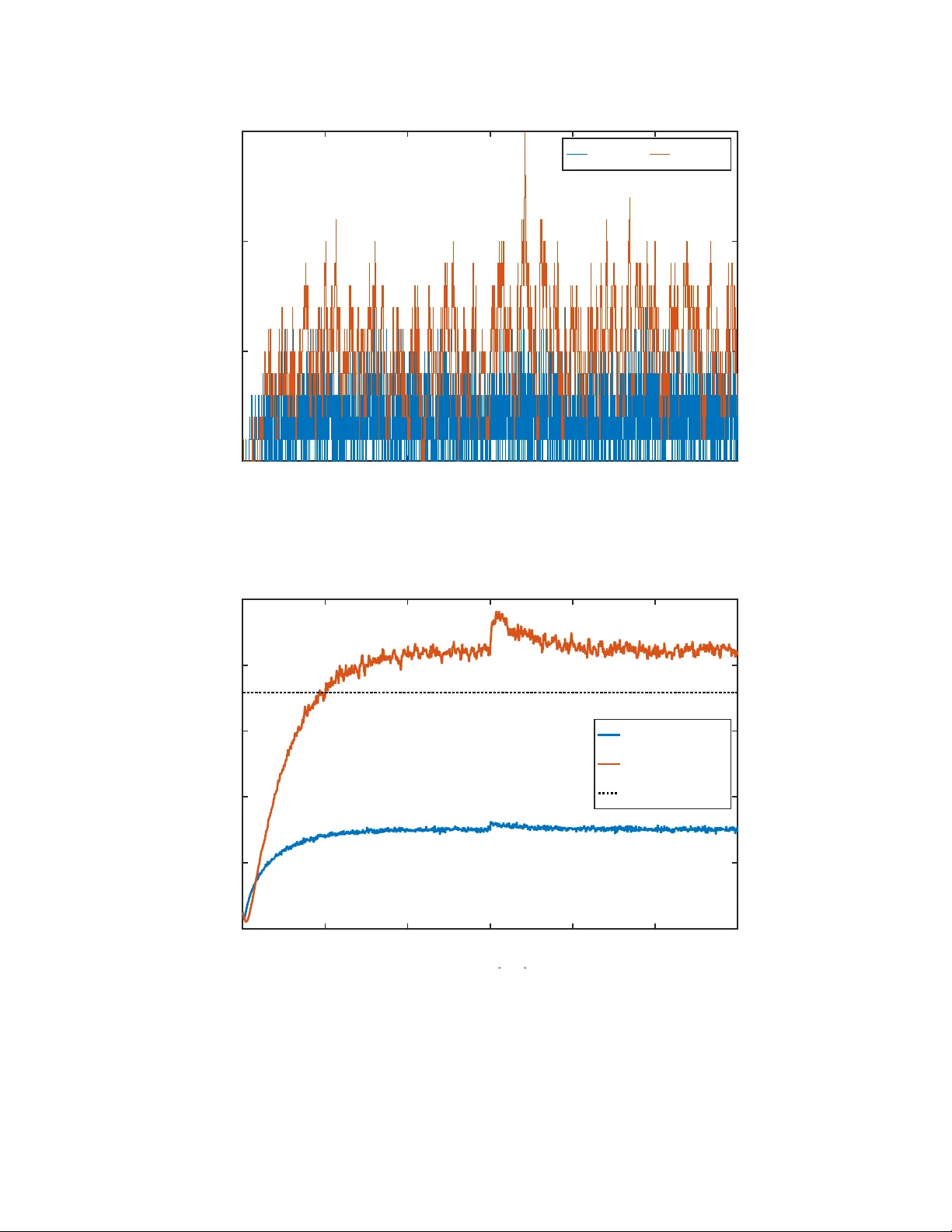
In-Silico Prop ortional-In tegral Momen t Con trol of Sto c hastic Gene Expression Coren tin Briat and Mustafa Khammash ∗ D-BSSE, ETH-Z ¨ uric h Abstract The problem of controlling the mean and the v ariance of a species of interest in a simple gene expression is addressed. It is sho wn that the protein mean level can be globally and robustly track ed to any desired v alue using a simple PI controller that satisfies certain sufficient conditions. Controlling b oth the mean and v ariance ho wev er requires an additional control input, e.g. the mRNA degradation rate, and lo cal robust trac king of mean and v ariance is prov ed to be ac hiev able using multiv ariable PI con trol, provided that the reference p oin t satisfies necessary conditions imposed b y the system. Ev en more importantly , it is shown that there exist PI con trollers that lo cally , robustly and sim ultaneously stabilize all the equilibrium p oin ts inside the admissible region. The results are then extended to the mean control of a gene expression with protein dimerization. It is sho wn that the moment closure problem can b e circum ven ted without inv oking any momen t closure technique. Lo cal stabilization and conv ergence of the a verage dimer population to any desired reference v alue is ensured using a pure in tegral control la w. Explicit b ounds on the con troller gain are provided and sho wn to b e v alid for an y reference v alue. As a byproduct, an explicit upp er-bound of the v ariance of the monomer sp ecies, acting on the system as unknown input due to the moment op enness, is obtained. The results are illustrated b y simulation. Keywor ds. Cyb er genetics; opto genetics; in-silic o c ontr ol; c el l p opulations; sto chastic r e action networks; r obustness 1 In tro duction The regulation problem of single-cells and the regulation problem of cell p opulations hav e at- tracted a lot of attention in recent y ears b ecause of their p oten tial in applications such as in bioreactors [1, 2], disease treatment (homeostasis restoring [3]), etc. V arious wa ys for con trolling single cells or cell p opulations exist. Among these is the so-called in-viv o con trol where controllers are implemented inside cells using biological elemen ts (genes, RNA, proteins, etc.) using synthetic biology and bio engineering techniques. Theoretical works hav e suggested that certain motifs could ac hieve p erfect adaptation for the controlled net work. Notably , circuits relying on an annihilation reaction of the con troller sp ecies hav e pro ven to be a credible solution to the regulation problem; see e.g. [4 – 8]. Other designs in volv e, for instance, phosphorylation cycles exhibiting an ultrasensitiv e b eha vior [9] or auto catalytic reactions [10, 11]. The alternative to in-viv o control is the so-called in-silico control in whic h con trol functions are mov ed outside the cells and are relegated to a digital ∗ email: corentin@briat,info; m ustafa.khammash@bsse.ethz.ch; url: www.briat.info; www.bsse.ethz.c h/ctsb 1 computer [12 – 17]. Actuation can b e p erformed using ligh t (optogenetics) or using chemical induc- ers (microfluidics) whereas measurements are mostly performed via the use of fluorescent molecules (suc h as the Green Fluorescent Protein – or GFP) whose cop y n umber can b e estimated using time-lapse microscop y or flow cytometry . In the current pap er, we fo cus on the in-silico control of cell p opulations in the momen ts equation framew ork, for which w e summarize and extend some of our previously obtained theoretical results. The pap er is divided in three parts. The first part is devoted to the con trol of the mean protein cop y n umber in a simple gene expression netw ork across a cell p opulation using a Prop ortional-In tegral (PI) control strategy . The considered con trol input is the transcription rate of the mRNA and the measured output is the mean of the protein cop y n umber across the cell p opulation. Note that this measure is p erfectly plausible as it can b e computed from the fluorescence (or the protein cop y n umber) distribution across the cell p opulation. As the output of a PI controller can b e negative, whic h w ould not correspond to an y meaningful control input here, w e resolv e this problem by placing an ON/OFF nonlinearity [18, 19] b etw een the controller and the system. Another solution to this problem is the use of an an tithetic integral con troller or p ositiv ely regularized integral con trollers; see e.g. [5, 20]. The lo cal exp onential stabilit y can b e easily prov en using a standard eigen v alue analysis, whereas the global asymptotic stabilit y is prov ed in the con text of absolute stabilit y using Popov’ criterion; see e.g. [21 – 23]. Additional results on the disturbance rejection, the robustness with delays and the generalization to arbitrary momen t equations are also given. The second part is dev oted to the extension of the abov e problem where, in addition to control- ling the protein mean, w e also aim at controlling the v ariance in the protein copy num b er across the cell p opulation. W e first show that a second con trol input, the degradation rate of the mRNA, needs to b e considered in order to able to indep enden tly con trol the mean and the v ariance of the protein cop y num b er across the cell p opulation. W e then identify the existence of a low er b ound for the stationary v ariance that cannot b e o vercome b y any in-silico control strategy using the momen ts as measured v ariables. This has to b e contrasted with what is achiev able using in-vivo con trol where the v ariance can be theoretically reduced b elo w this v alue [5, 24] b y suitably adjusting a negativ e feedback gain. Using the transcription rate and the degradation rate of the mRNA as con trol inputs, we demonstrate that a m ultiv ariable PI feedbac k can be used to locally and robustly trac k any desired protein mean and v ariance set-p oin t, pro vided this set-p oin ts satisfies a certain necessary condition imp osed by the structure of the system. The third and last part of the pap er is devoted to the control of the mean copy n umber of a protein dimer in a gene expression net work with protein dimerization. Although this ma y seem incremen tal, this netw ork exhibits a considerable increase in its complexity due to the dimerization . The main difficult y lies in the fact that the moments equations are no longer closed, which forces us to work with a momen t equation ha ving some unkno wn, yet p oten tially measurable, inputs. A second difficulty is that the moment equation b ecomes nonlinear, which increases the complexit y of the problem. A natural approach would b e to close the moments using some moment closure metho d (see e.g. [25]) and to con trol the closed moment equations. How ev er, b ecause of the inaccu- racy of moment closure sc hemes it is not guaranteed that the original moment equation will remain stable under the same conditions as the closed moments equation. W e prop ose here an alternative approac h whereby we exploit the ergo dicit y of the pro cess and solv e the control problem directly for the op en momen t equations where the v ariance of the protein cop y n umber acts as an input. W e show that this input is necessarily bounded by some v alue that w e explicitly c haracterize. Some lo cal asymptotic stability conditions are also obtained. This approach suggests that the momen t 2 equation op enness is not as problematic as in the sim ulation/analysis problem. Finally , simulated examples are given for illustration. Outline. Preliminary definitions and results are giv en in Section 2. The problem of con trolling the mean protein copy n umber in a gene expression netw ork is addressed in Section 3 whereas the problem of controlling b oth the mean and the v ariance in the protein copy num b er is considered in Section 4. Finally , the mean con trol of the dimer cop y n umber in a gene expression netw ork with dimerization is treated in Section 5. Examples are given in the related sections. Notations. The notation is prett y muc h standard. Given a random v ariable X , its exp ectation is denoted b y E [ X ]. F or a square matrix M , Sym[ M ] stands for the sum M + M ∗ . Given a vector v ∈ R n , the notation diag( v ) stands for a diagonal matrix having the elemen ts of v as diagonal en tries. 2 Preliminaries on sto c hastic reaction net w orks W e briefly introduce in this section sto chastic reaction netw orks as well as essential mo dels. F or more details, the readers are referred to [26]. A sto c hastic reaction net work is a system where N molecular sp ecies X 1 , . . . , X N in teract with each others through M reaction channels R 1 , . . . , R M . Eac h reaction R k is describ ed b y a propensity function w k : Z ≥ 0 7→ R ≥ 0 and a stoic hiometric v ector s k ∈ Z N . The propensity function w k is suc h that for all κ ∈ Z ≥ 0 suc h that κ + s k / ∈ Z ≥ 0 , we ha ve that w k ( κ ) = 0. Assuming homogeneous mixing, it can b e shown that the pro cess ( X 1 ( t ) , . . . , X N ( t )) t ≥ 0 is a Marko v pro cess that can b e describ ed by the so-called Chemical Master Equation (CME), or F orw ard Kolmogorov equation, given b y ˙ p κ 0 ( κ , t ) = M X k =1 [ w k ( κ − s k ) p κ 0 ( κ − s k , t ) − w k ( κ ) p κ 0 ( κ , t )] where p κ 0 ( κ , t ) = P [ X ( t ) = κ | X (0) = κ 0 ] and κ 0 is the initial condition. Based on the CME, dynamical expressions for the first- and second-order moments may b e easily deriv ed and are given b y d E [ X ( t )] dt = S E [ w ( X ( t ))] , d E [ X ( t ) X ( t ) T ] dt = Sym[ S E [ w ( X ( t )) X ( t ) T ]] + S diag { E [ w ( X ( t ))] } S T (1) where S :=  s 1 . . . s M  ∈ R N × M is the stoichiometry matrix and w ( κ ) :=  w 1 ( κ ) . . . w M ( κ )  T ∈ R M the v ector of prop ensit y functions. When the propensity functions are affine (i.e. w ( κ ) = W κ + w 0 , W ∈ R M × N , w 0 ∈ R M ), then the ab ov e system can b e rewritten in the form d E [ X ( t )] dt = S W E [ X ( t )] + S w 0 , d Σ( t ) dt = Sym[ S W Σ( t )] + S diag ( W E [ X ( t )] + w 0 ) S T (2) where Σ( t ) := E [( X ( t ) − E [ X ( t )])( X ( t ) − E [ X ( t )]) T ] is the cov ariance matrix. An immediate prop ert y of (2) is that it forms a closed system, unlike in the more general case (1) where the first 3 and second order moments dep end on higher-order ones whenever the prop ensit y functions are of mass-action. 3 Mean con trol of protein lev els in a gene expression net w ork The ob jectiv e of the current section is to give a clear picture of the mean control of the n umber of proteins using a simple p ositive PI c ontr ol ler , i.e. a PI controller generating nonnegativ e control inputs. The considered control input is the transcription rate k r whic h can b e externally actuated using, for instance, light-induced transcription [12]. It is sho wn in this section that a p ositiv e PI con trol law allows to ac hieve global and robust output trac king of the mean n umber of proteins. 3.1 Preliminaries W e consider in this section the follo wing mo del for gene expression R 1 : ∅ k r − → X 1 , R 2 : X 1 γ r − → ∅ , R 3 : X 1 k p − → X 1 + X 2 , R 4 : X 2 γ p − → ∅ (3) where X 1 denotes the mRNA and X 2 the asso ciated protein. In v ector form, the equations (2) rewrite       ˙ x 1 ( t ) ˙ x 2 ( t ) ˙ x 3 ( t ) ˙ x 4 ( t ) ˙ x 5 ( t )       =  A ee 0 A σ e A σ σ        x 1 ( t ) x 2 ( t ) x 3 ( t ) x 4 ( t ) x 5 ( t )       +  B e B σ  k r (4) where the state v ariables are defined by x i := E [ X i ], i = 1 , 2, x 3 := V ( X 1 ), x 4 := Cov( X 1 , X 2 ), x 5 := V ( X 2 ), and the system matrices by A ee =  − γ r 0 k p − γ p  , A σ e =   γ r 0 0 0 k p γ p   , B e =  1 0  , A σ σ =   − 2 γ r 0 0 k p − ( γ r + γ p ) 0 0 2 k p − 2 γ p   , B σ =   1 0 0   , (5) where k r > 0 is the transcription rate of DNA in to mRNA, γ r > 0 is the degradation rate of mRNA, k p > 0 is the translation rate of mRNA into protein and γ p > 0 is the degradation rate of the protein. W e consider here the follo wing restriction of system (4):  ˙ x 1 ( t ) ˙ x 2 ( t )  = A ee  x 1 ( t ) x 2 ( t )  + B e u ( t ) (6) and the p ositive PI con trol law u ( t ) = ϕ  k 1 ( µ ∗ − x 2 ( t )) + k 2 Z t 0 [ µ ∗ − x 2 ( s )] ds  (7) 4 where µ ∗ is the mean num b er of protein to track and the scalars k 1 , k 2 the gains of the controller. The nonlinearity ϕ ( · ) can either b e an ON/OFF nonlinearity ϕ ( u ) := max { 0 , u } [19] or a saturated ON/OFF one ϕ ( u ) := min { max { 0 , u } , ¯ u } where ¯ u > 0 is the maximum admissible v alue for the con trol input. Prop ert y 1 Given a c onstant r efer enc e µ ∗ ≥ 0 , the e quilibrium p oint of the system (6)-(7) is given by x ∗ 2 = µ ∗ and x ∗ 1 = µ ∗ γ p k p , u ∗ = µ ∗ γ p γ r k p and I ∗ = u ∗ k 2 (8) wher e I ∗ is the e quilibrium value of the inte gr al term. When a satur ate d ON/OFF nonline arity is use d, for this e quilibrium p oint to b e me aningful, we ne e d that u ∗ ≤ ¯ u . As expected, the in tegrator allo ws to ac hieve constant set-p oin t trac king for the mean protein coun t regardless the v alues of the parameters of the system. 3.2 Lo cal stabilizability , stabilization and output trac king Since the equilibrium control input u ∗ and the set-point µ ∗ are b oth p ositive, the nonlinearit y ϕ ( · ) is not active in a sufficiently small neighborho o d of the equilibrium point (8). The ON/OFF nonlinearit y can hence b e lo cally ignored and the local analysis performed on the corresp onding linear system. Assuming first that the system parameters k p , γ p , γ r are exactly known, the following result on lo cal nominal stabilizabilit y and stabilization is obtained: Lemma 2 Given system p ar ameters k p , γ p , γ r > 0 , the system (6) is lo c al ly stabilizable using the c ontr ol law (7). Mor e over, the e quilibrium p oint (8) of the close d-lo op system (6)-(7) is lo c al ly asymptotic al ly (exp onential ly) stable if and only if the c onditions µ ∗ γ p γ r k p ≤ ¯ u, k 1 > k 2 γ p + γ r − γ p γ r k p , and k 2 > 0 (9) hold. M Pr o of : The closed-lo op system (6)-(7) is given by   ˙ x 1 ( t ) ˙ x 2 ( t ) ˙ I ( t )   =   − γ r − k 1 k 2 k p − γ p 0 0 − 1 0     x 1 ( t ) x 2 ( t ) I ( t )   +   k 1 0 1   µ ∗ (10) where I is the integrator state of the con troller. Lo cal stabilizabilit y is then equiv alent to the ex- istence of a pair ( k 1 , k 2 ) ∈ R 2 suc h that the state matrix of the augmented system (10) is Hurwitz stable, i.e. has p oles in the op en left-half plane. The Routh-Hurwitz criterion yields the conditions (9) that define a nonempty subset of the plane ( k 1 , k 2 ). System (6) is hence locally stabilizable using the PI control la w (7) for any triplet of parameter v alues ( k p , γ r , γ p ) ∈ R 3 > 0 . As a consequence, the closed-lo op system is lo cally asymptotically stable when the con trol parameters are lo cated inside the stabilit y region defined b y the conditions (9). ♦ In order to extend the abov e result to the uncertain case, w e assume here that the system parameters ( k p , γ p , γ r ) b elong to the set P µ := [ k − p , k + p ] × [ γ − p , γ + p ] × [ γ − r , γ + r ] (11) 5 where the parameter bounds k − p ≤ k + p , γ − p ≤ γ + p and γ − r ≤ γ + r are real p ositiv e n umbers. W e then obtain the following result: Lemma 3 The system (6) with unc ertain c onstant p ar ameters ( k p , γ p , γ r ) ∈ P µ is r obustly lo c al ly asymptotic al ly (exp onential ly) stabilizable using the c ontr ol law (7). Mor e over, the e quilibrium p oint (8) of the close d-lo op system (6)-(7) is lo c al ly r obustly asymptotic al ly (exp onential ly) stable if and only if the c onditions µ ∗ γ + p γ + r k − p ≤ ¯ u, k 1 > k 2 γ − p + γ − r − γ − r γ − p k + p , and k 2 > 0 (12) hold. When ¯ u = ∞ , then γ + p and γ + r c an b e arbitr arily lar ge and k − p c an b e arbitr arily smal l. M Pr o of : The starting p oint is the lo w er b ound for k 1 obtained in Lemma 2 given b y f ( x, y , z ) := k 2 y + z − y z x , x, y , z , k 2 > 0 and let ¯ f := sup ( x,y ,z ) ∈P µ f ( x, y , z ) suc h that µ ∗ y z /x ≤ ¯ u for all ( x, y , z ) ∈ P µ . Simple calculations sho w that f ( x, y , z ) is increasing in x and decreasing in y , z ov er ( x, y , z ) ∈ P µ . Hence, we ha ve ¯ f = f ( k + p , γ − p , γ − r ) and k 1 > ¯ f implies that k 1 > f ( x, y , z ) for all ( x, y , z ) ∈ P µ . This concludes the pro of. ♦ 3.3 Global stabilizability , stabilization and output tracking Lo cal prop erties obtained in the previous section are generalized here to global ones. Noting first that the nonlinear function ϕ ( · ) is time-inv ariant and b elongs to the sector [0 , 1], i.e. 0 ≤ ϕ ( x ) /x ≤ 1, x ∈ R , stability can then b e analyzed using absolute stabilit y theory [27] and an extension of the P op o v criterion [21, 27] for marginally stable systems [28, 29]. W e hav e the follo wing result: Theorem 4 Given system p ar ameters k p , γ p , γ r > 0 , then the e quilibrium p oint (8) of the close d- lo op system (6)-(7) is glob al ly asymptotic al ly stable if u ∗ ≤ ¯ u , the c onditions (9) hold and one of the fol lowing statements hold for some q > 0 (a) z 0 ( q ) > 0 and z 1 ( q ) > 0 , or (b) z 0 ( q ) > 0 , z 1 ( q ) < 0 and z 1 ( q ) 2 − 4 z 0 ( q ) < 0 wher e z 0 ( q ) = γ 2 r γ 2 p + k p [ γ r ( γ p k 1 − k 2 + γ p k 2 q ) − γ p k 2 ] z 1 ( q ) = γ 2 p + γ 2 r + k p [( k 1 ( γ p + γ r ) − k 2 ) q − k 1 ] . M (13) Pr o of : Accordingly to the absolute stabilit y paradigm, the closed-lo op system (6)-(7) is rewritten as the ne gative in terconnection of the marginally stable L TI system H ( s ) = k p ( k 1 s + k 2 ) s ( s + γ r )( s + γ p ) (14) and the static nonlinearit y ϕ ( · ); i.e. u = − ϕ ◦ H u . W e assume in the follo wing that k 2 > 0, whic h is a necessary condition for lo cal asymptotic stabilit y of the equilibrium point (8). Since lim s → 0 sH ( s ) = k p k 2 γ r γ p > 0, then the Popov criterion [21, 29] can b e applied. It state s that system (6) 6 is absolutely stabilizable using control ler (7) if there exist ( k 1 , k 2 ) ∈ R 2 and q ≥ 0 such that the condition F ( j ω, q ) := < [(1 + q j ω ) H ( j ω )] > − 1 (15) holds for all ω ∈ R . In order to chec k this condition, first rewrite F ( j ω , q ) as F ( j ω, q ) = N 0 ( ω ) D ( ω ) + q N 1 ( ω ) D ( ω ) (16) where N 0 ( ω ) = k p  k 1 ( γ r γ p − ω 2 ) − k 2 ( γ r + γ p )  N 1 ( ω ) = k p  k 1 ω 2 ( γ r + γ p ) + k 2 ( γ p γ r − ω 2 )  D ( ω ) = ( ω 2 + γ 2 r )( ω 2 + γ 2 p ) . (17) Since D ( ω ) > 0 for all ω ∈ R , then the condition (15) is equiv alent to N 0 ( ω ) + q N 1 ( ω ) + D ( ω ) > 0 for all ω ∈ R . Letting ¯ ω := ω 2 , w e get Z ( ¯ ω ) := ¯ ω 2 + z 1 ( q ) ¯ ω + z 0 ( q ) > 0 for all ¯ ω ∈ [0 , ∞ ) and where z 0 ( q ) and z 1 ( q ) are as in (13). The problem therefore essentially becomes a p ositivit y analysis of the p olynomial Z ( ¯ ω ) ov er [0 , ∞ ). This p olynomial is p ositive if and only if either z 0 ( q ) > 0 and z 1 ( q ) > 0 or z 0 ( q ) > 0, z 1 ( q ) < 0 and z 1 ( q ) 2 − 4 z 0 ( q ) < 0. T o pro v e global asymptotic stabilit y , it is enough to note that since u ∗ > 0, we hav e ϕ ( u ∗ ) = u ∗ and the con trol input equilibrium v alue do es not lie in the k ernel of ϕ . According to [29], this allo ws to conclude on the global asymptotic stabilit y of the equilibrium p oin t (8). The pro of is complete. ♦ As the conditions of Theorem 4 are implicit in nature, w e provide here some more useful conditions Corollary 5 Given system p ar ameters k p , γ p , γ r > 0 , then the e quilibrium p oint (8) of the close d- lo op system (6)-(7) is glob al ly asymptotic al ly stable if the fol lowing c onditions µ ∗ γ p γ r k p ≤ ¯ u, k 1 > k 2 γ p + γ r and k 2 > 0 (18) hold. M Pr o of : This result can b e prov en by noticing that when b oth the conditions k 2 > 0 and k 1 ( γ p + γ r ) − k 2 > 0 hold, then z 0 ( q ) and z 1 ( q ) can b oth b e made positive provided that q ≥ 0 is c hosen s ufficien tly large, proving then that the equilibrium p oin t (8) is globally stable when these conditions are met. ♦ Remark 6 It is inter esting to note that the lo c al and glob al stability c onditions c oincides in the limit k p → ∞ . This suggests that when the DC-gain of the system incr e ases, the glob al c onditions b e c ome less and less c onservative. Note, however, that the c onditions ar e likely to b e c onservative due to the fact that the se ctor nonline arity includes ne gative values as wel l as any other typ e of nonline arity within that se ctor. It is immediate to obtain the following extension to the uncertain case: Lemma 7 Given system p ar ameters ( k p , γ p , γ r ) ∈ P µ , then the e quilibrium p oint (8) of the close d- lo op system (6)-(7) is glob al ly r obustly asymptotic al ly stable if the fol lowing c onditions µ ∗ γ + p γ + r k − p ≤ ¯ u, k 1 > k 2 γ − p + γ − r , and k 2 > 0 (19) hold. When ¯ u = ∞ , then γ + p and γ + r c an b e arbitr arily lar ge and k − p c an b e arbitr arily smal l. M 7 3.4 Generalization of the global result to any momen t equation W e consider here an arbitrary momen t equation ˙ x ( t ) = Ax ( t ) + B u ( t ) y ( t ) = C x ( t ) (20) where A ∈ R n is Metzler, B ∈ R n × m ≥ 0 and C ∈ R m × n ≥ 0 . W e also assume that w e ha ve as many PI con trollers than input/output pairs and that u ( t ) = ϕ  K 1 ( µ ∗ − y ( t )) + K 2 Z t 0 ( µ ∗ − y ( s )) ds  (21) where K 1 and K 2 are the (matrix) gains of the controller. W e ha ve the following result: Theorem 8 L et us c onsider the moment e quation (20) with the c ontr ol lers (21) and assume that the set-p oint ( µ 1 ∗ , . . . , µ m ∗ ) is achievable (i.e. ther e is a p ositive u ∗ ≤ ¯ u such that y ∗ = µ ∗ ). Then, the unique e quilibrium p oint of the close d-lo op system (20) - (21) is glob al ly asymptotic al ly stable if ther e exist a p ositive semidefinite matrix N and an invertible matrix Z such that Sym[ I m + ( I m + j ωN ) Z G ( j ω ) Z − 1 ] > 0 for all ω ∈ R (22) wher e G ( s ) = ( K 1 + K 2 /s ) C ( sI − A ) − 1 B . A lternatively, this is e quivalent to the existenc e of symmetric p ositive definite r e al matric es P and Γ and a symmetric p ositive semidefinite matrix ¯ N such that the matrix  A T a P + P A a P B a − C T a Γ − ( ¯ N C a A a ) T ? − 2Γ − Sym[ ¯ N C a B a ]  (23) is ne gative definite wher e  A a B a C a 0  =   A 0 B C 0 0 K 1 C K 2 0   . (24) Pr o of : This follo ws from the multiv ariable Popov criterion with the use of scalings (see e.g. [30]). The LMI condition can b e obtained by noticing that the frequency domain condition is equiv alen t to saying that the system I m + ( I m + sN ) Z G ( s ) Z − 1 is strictly p ositive real. F rom the Kalman- Y akub o vich-P op o v Lemma, this is equiv alen t to saying that the matrix  A T a P + P A a P B Z − 1 − ( Z C a + ¯ N Z C a A a ) T ? − 2Γ − Sym[ ¯ N Z C a B a Z − 1 ]  (25) is negativ e definite. P erforming a congruence transformation with respect to the matrix diag( I n , Z ) yields the condition (23) where w e hav e used the changes of v ariables ¯ N = Z T N Z and Γ = Z T Z . The pro of is completed. ♦ While it ma y be difficult to analytically chec k these conditions in the general case, they can b e n umerically chec k ed using semidefinite programming [31]. Note, ho wev er, that when the gains K 1 and K 2 of the con troller are not fixed a priori, then the problem becomes non linear and ad-ho c iterativ e metho ds may need to b e considered to find suitable gains. Note that this problem relates to the design of a static output feedbac k con troller, some instances b eing kno wn to b e NP-hard [32]. 8 3.5 Input disturbance rejection It seems imp ortan t to discuss disturbance rejection prop erties of the closed-lo op system. F or instance, basal transcription rates can b e seen as constan t input disturbances that need to b e rejected. Ho wev er, because of the p ositivit y requirement for the con trol input, the rejection of constan t input disturbances is only p ossible when they remain within certain b ounds. Lemma 9 Given system p ar ameters k p , γ p , γ r > 0 , the c ontr ol law (7) glob al ly r eje cts c onstant input disturb anc es δ u that satisfy γ p γ r k p µ ∗ − ¯ u ≤ δ u ≤ γ p γ r k p µ ∗ (26) pr ovide d that the c ontr ol ler gains satisfy c onditions (18). M Pr o of : In presence of constant input disturbances, the equilibrium v alue of the control input is giv en by u ∗ δ := γ p γ r k p µ ∗ − δ u . (27) This v alue needs to b e nonnegativ e in order to b e driven b y the on-off nonlinearity ϕ , whic h is the case if and only if condition (26) holds. ♦ The ab o v e result readily extends to the uncertain case: Lemma 10 Assume ( k p , γ p , γ r ) ∈ P µ , the c ontr ol law (7) satisfying c onditions (19) glob al ly and r obustly r eje cts c onstant input disturb anc es if and only if the c ondition γ + p γ + r k − p µ ∗ − ¯ u ≤ δ u ≤ γ − p γ − r k + p µ ∗ (28) is fulfil le d. M Pr o of : The pro of follows from a simple extremum argumen t similar to the one used in the pro of of Lemma 3. ♦ It seems imp ortant to p oin t out that the sets of admissible p erturbations defined b y (26) or (28) do not dep end on the choice for the controller gains. They do, ho wev er, dep end on the mean reference v alue µ ∗ , which is exp ected since small µ ∗ ’s yield small control inputs whic h are more lik ely to b e o verwhelmed by disturbances. 3.6 Lo cal robustness with resp ect to constan t input dela y Let us consider now that the con trol input is dela yed b y some constant dela y h > 0. In this case, it is conv enient to rewrite the closed-lo op system according to the state v ariable ( x 1 , x 2 , u ):   ˙ x 1 ( t ) ˙ x 2 ( t ) ˙ u ( t )   =   − γ r 0 0 k p − γ p 0 − k 1 k p k 1 γ p − k 2 0     x 1 ( t ) x 2 ( t ) u ( t )   +   0 0 1 0 0 0 0 0 0     x 1 ( t − h ) x 2 ( t − h ) u ( t − h )   +   0 0 k 2   µ ∗ . (29) 9 W e already kno w that the system can be made stable when h = 0. In tuitively , the delay will deteriorate the stability of the system since it will b e con trolled with past information instead of curren t one. This leads to the following result: Prop osition 11 Assume that the gains k 1 and k 2 ar e given and satisfy the c onditions of L emma 2. Then, the system (29) is asymptotic al ly stable for al l h ∈ [0 , h c ) and unstable otherwise wher e h c := − 1 ω c arg  − j ω c ( j ω c + γ r )( j ω c + γ p ) k p ( k 1 j ω c + k 2 )  (30) wher e ω c is the only p ositive solution to the algebr aic e quation Φ( ω ) := ω 6 + ( γ 2 p + γ 2 r ) ω 4 + ( γ 2 r γ 2 p − k 2 p k 2 1 ) ω 2 − k 2 p k 2 2 = 0 . M Pr o of : This result can b e pro ven using a standard ro ot analysis of the characteristic equation. T o this aim, define the characteristic equation of the closed-lo op system as K ( s, h ) := P ( s ) + e − sh Q ( s ) where P ( s ) := s ( s + γ r )( s + γ p ) and Q ( s ) := k p ( k 1 s + k 2 ). There exists a pair of complex conjugate ro ot on the imaginary axis for K ( s, h ) iff D ( j ω , h ) = 0 for some ω > 0. This is equiv alen t to sa ying that | P ( j ω ) | 2 − | Q ( j ω ) | 2 = 0. Calculations show that the equality | P ( j ω ) | 2 − | Q ( j ω ) | 2 coincides with Φ( ω ). T o study the existence of p ositiv e solutions to the algebraic equation Φ( ω ) = 0, w e can alternativ ely consider the third-order algebraic equation Φ( ω 1 / 2 ) = 0. In v oking then Descartes’ rule of sign, the num b er of sign c hanges in the co efficien ts is alw ays 1, meaning that b oth Φ( ω ) = 0 and Φ( ω 1 / 2 ) = 0 hav e one and only one positive solution, whic h we denoted by ω c . Let us then define ( ω c , h c ) to b e the pair for which K ( j ω c , h c ) = 0. Then, we get that e − j ω c h c = − P ( j ω c ) /Q ( j ω c ) and hence h c is giv en by (30). ♦ 3.7 Example F or sim ulation purposes, we consider the normalized version of system (4) tak en from [12] and giv en b y: ˙ ¯ x 1 ( t ) = − ( γ 0 r + u 2 ) ¯ x 1 ( t ) + ˜ u 1 ( t ) ˙ ¯ x 2 ( t ) = γ p ( ¯ x 1 ( t ) − ¯ x 2 ( t )) ˙ ¯ x 3 ( t ) = ( γ 0 r + u 2 ( t )) ¯ x 1 ( t ) − 2( γ 0 r + u 2 ) ¯ x 3 ( t ) + ˜ u 1 ( t ) ˙ ¯ x 4 ( t ) = ( γ 0 r + γ p ) ¯ x 3 ( t ) − ( γ 0 r + u 2 + γ p ) ¯ x 4 ( t ) ˙ ¯ x 5 ( t ) = γ p α [ ¯ x 1 ( t ) + ¯ x 2 ( t ) + 2( α − 1) ¯ x 4 ( t )] − 2 γ p ¯ x 5 ( t ) (31) where ˜ u 1 ( t ) = γ 0 r + bu 1 ( t ), γ 0 r = 0 . 03, γ p = 0 . 0066, b = 0 . 9587, k p = 0 . 06 and α = 1 + k p / ( γ 0 r + γ p ). The system has been normalized according to basal lev els for transcription rate k 0 r and degradation rate γ 0 r . In the absence of con trol inputs, i.e. ˜ u 1 ≡ 0 and u 2 ≡ 0, the system conv erges to the normalized equilibrium v alues ¯ x ∗ i = 1, i = 1 , . . . , 5. The parameter v alues are b orro w ed from [12]. F or this system, the global stabilit y conditions write γ 0 r ( µ − 1) b ≤ ¯ u, k 1 > k 2 γ p + γ 0 r , k 2 > 0 . (32) W e choose ¯ u = ∞ , k 1 = 0 . 1191 and k 2 = 0 . 0007, whic h satisfy the ab o v e conditions. Sim ulations yield the tra jectories of Fig. 1 and Fig. 2. W e can see, as exp ected, that the prop osed controller ac hieves output tracking for differen t references and in presence of a saturation on the input, although conv ergence tak es longer in the latter case. 10 0 100 200 300 400 500 600 1 2 3 4 5 6 7 8 9 Figure 1: T ra jectories of the mean num b er of proteins for differen t reference v alues. 3.8 Concluding remarks The protein v ariance at equilibrium is giv en by σ 2 ∗ = µ ∗  1 + k p γ p + γ r  (33) whic h sho ws that the equilibrium v ariance dep ends linearly on the mean. Therefore, it cannot be indep enden tly assigned to a desired v alue. W e can also observe that a higher mean yields a higher v ariance, which motiv ates the aim of controlling the v ariance in order to keep it at a desired lev el. 4 Mean and V ariance con trol of protein lev els in a gene expression net w ork As discussed in the previous section, acting on k r is not sufficient for controlling b oth the mean and v ariance equilibrium v alues. It is shown in this section that v ariance control can b e achiev ed b y adding the second con trol input γ r ≡ u 2 . F undamental limitations of the con trol system are discussed first, then lo cal stabilizabilit y is addressed. 4.1 F undamental limitations Let us consider in this section the control inputs k r ≡ u 1 and γ r ≡ u 2 . It is sho wn b elo w that there is a fundamental limitation on the references v alues for the mean and v ariance. 11 0 200 400 600 800 1000 1200 1 2 3 4 5 6 7 8 9 10 Figure 2: T ra jectories of the mean n umber of proteins for different reference v alues and with a saturation of ¯ u = 0 . 3. Prop osition 12 The set of admissible r efer enc e values ( µ ∗ , σ 2 ∗ ) is given by the op en and nonempty set A :=  ( x, y ) ∈ R 2 > 0 : x < y <  1 + k p γ p  x  (34) wher e k p , γ p > 0 . M Pr o of : The low er b ound is imp osed by the co efficien t of v ariation which gives σ 2 ∗ =  1 + k p γ r + γ p  µ ∗ > µ ∗ . (35) The upp er b ound is imp osed by the p ositivit y of the unique equilibrium control inputs v alues giv en b y u ∗ 1 = γ p k p µ ∗ u ∗ 2 and u ∗ 2 = − γ p + k p µ ∗ σ 2 ∗ − µ ∗ (36) whic h are well-posed since σ 2 ∗ − µ ∗ > 0 according to the co efficien t of v ariation constraint. The second equilibrium con trol input v alue u ∗ 2 is p ositiv e if and only if σ 2 ∗ <  1 + k p γ p  µ ∗ , which in turn implies that u ∗ 1 is nonnegativ e as well. The pro of is complete. ♦ The low er bound obtained abov e remains v alid when k p or γ p are chosen as second con trol in- puts. The factor of the upp er-bound ho wev er c hanges to 1 + k p /γ r when γ p ≡ u 2 , or b ecomes unconstrained when k p ≡ u 2 . Note ho wev er that the upp er b ound on the v ariance is not a strong limitation in itself b ecause w e are mostly interested in ac hieving low v ariance. Note also that since the low er b ound on the achiev able v ariance is indep enden t of the controller structure, it is hence p ointless to lo ok for adv anced control tec hniques in view of improving this limit. 12 A p ositiv e fact, ho wev er, is that the low er b ound is fixed and do es not depend on the knowledge of the parameters of the system. This p otentially mak es lo w equilibrium v ariance robustly achiev able. 4.2 Problem formulation Considering the con trol inputs k r ≡ u 1 and γ r ≡ u 2 , the system (4) can b e rewritten as the bilinear system ˙ x 1 = − u 2 x 1 + u 1 ˙ x 2 = k p x 1 − γ p x 2 ˙ x 3 = u 2 x 1 − 2 u 2 x 3 + u 1 ˙ x 4 = k p x 3 − γ p x 4 − u 2 x 4 ˙ x 5 = k p x 1 + γ p x 2 + 2 k p x 4 − 2 γ p x 5 ˙ I 1 = µ ∗ − x 2 ˙ I 2 = σ 2 ∗ − x 5 (37) where I 1 and I 2 are the states of the integrators. The control inputs are defined as the outputs of a m ultiv ariable p ositive PI con troller u 1 = ϕ 1 ( k 1 e 1 + k 2 I 1 + k 3 e 2 + k 4 I 2 ) u 2 = ϕ 2 ( k 5 e 1 + k 6 I 1 + k 7 e 2 + k 8 I 2 ) (38) where e 1 := µ ∗ − x 2 , e 2 := σ 2 ∗ − x 5 , and ϕ i ( · ) := min { max { 0 , ·} , ¯ u i } , ¯ u i > 0, i = 1 , 2. Prop ert y 13 Assume that k 2 k 8 − k 4 k 6 6 = 0 , then the e quilibrium p oint of the system (37)-(38) is unique and given by x ∗ 1 = γ p k p µ ∗ , x ∗ 2 = µ ∗ , x ∗ 3 = x ∗ 1 , x ∗ 4 = γ p γ p + u ∗ 2 µ ∗ , x ∗ 5 = σ 2 ∗ , u ∗ 1 = γ p k p µ ∗ u ∗ 2 , u ∗ 2 = − γ p + k p µ ∗ σ 2 ∗ − µ ∗ (39) and  I ∗ 1 I ∗ 2  =  k 2 k 4 k 6 k 8  − 1  u ∗ 1 u ∗ 2  (40) pr ovide d that u ∗ i ≤ ¯ u i , i = 1 , 2 . Asso ciated with the set of admissible references A , we define the set of equilibrium p oin ts as X ∗ :=  ( x ∗ , I ∗ ) ∈ R 7 : ( y ∗ , σ 2 ∗ ) ∈ A , u ∗ i ∈ [0 , ¯ u i ] , i = 1 , 2  . 4.3 Lo cal stabilizability and stabilization Since the equilibrium con trol inputs are p ositiv e, the nonlinearities are not active in a neigh b or- ho od of the equilibrium p oin t (39)-(40). Lo cal analysis can hence b e performed using standard linearization tec hniques. The corresp onding Jacobian system is given by ˙ x ` = A ∗ ` x ` (41) 13 where A ∗ ` is giv en by                 γ p + k p µ ∗ δ − k 1 + γ p k 5 µ ∗ k p 0 0 − k 3 + γ p k 7 µ ∗ k p k 2 − γ p k 6 µ ∗ k p k 4 − γ p k 8 µ ∗ k p k p − γ p 0 0 0 0 0 − γ p − k p µ ∗ δ − k 1 + γ p k 5 µ ∗ k p 2 γ p + 2 k p µ ∗ δ 0 − k 3 + γ p k 7 µ ∗ k p k 2 − γ p k 6 µ ∗ k p k 4 − γ p k 8 µ ∗ k p 0 − k 5 γ p δ k p k p k p µ ∗ δ − γ p k 7 δ k p γ p k 6 δ k p γ p k 8 δ k p k p γ p 0 2 k p − 2 γ p 0 0 0 − 1 0 0 0 0 0 0 0 0 0 − 1 0 0                 (42) with δ := µ ∗ − σ 2 ∗ . The follo wing result states conditions for the Jacobian system to b e locally represen tative of the b eha vior of the original nonlinear system: Lemma 14 The Jac obian system ful ly char acterizes the lo c al b ehavior of the c ontr ol le d nonline ar system (37)-(38) if and only if the c ondition k 2 k 8 − k 4 k 6 6 = 0 holds. M Pr o of : F or the Jacobian system to represen t the lo cal b eha vior, it is necessary and sufficient that A ∗ ` has no eigenv alue at 0. A quick c heck at the determinant v alue det( A ∗ ` ) = 4 γ p k p ( k 2 k 8 − k 4 k 6 )( µ ∗ ( k p + γ p ) − γ p σ 2 ∗ ) yields that the condition k 2 k 8 − k 4 k 6 6 = 0 is necessary and sufficien t for the lo cal representativit y of the nonlinear system. Note that since ( µ ∗ , σ 2 ∗ ) ∈ A , the term µ ∗ ( k p + γ p ) − γ p σ 2 ∗ is alw ays different from 0. The pro of is complete. ♦ The lo cal system b eing linear, the Routh-Hurwitz criterion could ha ve indeed b een applied as in the mean control case, but would hav e led to quite complex algebraic inequalities, difficult to analyze in the general case, ev en for simple controller structures. Despite the ‘large size’ of the matrix A ∗ ` , it is fortunately still p ossible to provide a stabilizabilit y result using the fact that A ∗ ` is marginally stable when the controller parameters k i are set to 0. This is obtained using p erturbation theory of nonsymmetric matrices [33]. Lemma 15 Given any k p , γ p > 0 , the biline ar system (37) is lo c al ly asymptotic al ly stabilizable ar ound any e quilibrium p oint (39)-(40) using the c ontr ol law (38) pr ovide d that ( µ ∗ , σ 2 ∗ ) ∈ A and u ∗ i ≤ ¯ u i , i = 1 , 2 . M Pr o of : The p erturbation argumen t [33, Theorem 2.7] relies on c hecking whether the eigenv alues on the imaginary axis can b e shifted by sligh tly p erturbing the controller co efficien ts around the ‘0-con troller’, i.e. b y letting k i = ε d i , where ε ≥ 0 is the small p erturbation parameter and d i is the perturbation direction corresp onding to the con troller parameter k i . W e assume here that b oth in tegrators are in volv ed in the controller, that is | d 2 | + | d 6 | > 0 and | d 4 | + | d 8 | > 0. T o pro ve the result, let us first rewrite the matrix A ∗ ` as A ∗ ` = A 0 + ε 8 X j =1 d j A j . The matrix A 0 is a marginally stable matrix with a semisimple eigen v alue of multiplicit y tw o at zero. P aradoxically , these eigen v alues in tro duced b y the PI controller are the only critical ones that must b e stabilized, 14 i.e. shifted to the op en left-half plane. F rom p erturbation theory of general matrices [33], it is kno wn that semisimple eigenv alues bifurcate in to (distinct or not) eigenv alues according to the expression [33] λ i ( ε, d ) = ε ξ i ( d ) + o ( ε ), i = 1 , 2 where ξ i ( d ) is the i th eigen v alue of the matrix M ( d ) := 8 X j =1 d j ν ` A j ν r where ν ` ∈ R 2 × 5 and ν r ∈ R 5 × 2 denote the normalized left- and right- eigen vectors 1 asso ciated with the semisimple zero eigen v alue. It turns out that all ν ` A j ν r ’s with o dd index are zero, indicating that the proportional gains ha ve a locally negligible stabilizing effect. This hence reduces the size of the problem to 4 parameters, i.e. those related to integral terms. W e mak e no w the additional restriction that d 4 = d 6 = 0 reducing the con troller structure to one in tegrator p er control channel. The matrix M ( d ) then b ecomes M ( d ) = ψ     k p d 2 γ p − d 8 µ ∗ k p σ 2 ∗ d 2 γ p µ ∗ γ p ( µ ∗ − σ 2 ∗ ) 2 k p µ ∗ + µ ∗ − 2 σ 2 ∗     where ψ := µ ∗ − σ 2 ∗ γ p ( µ ∗ − σ 2 ∗ ) + k p µ ∗ . The zero semisimple eigen v alues then mov e to the op en left-half plane if there exist p erturbation directions d 2 , d 8 ∈ R , d 2 d 8 6 = 0, such that M ( d ) is Hurwitz stable. W e can now in vok e the Routh-Hurwitz criterion on M ( d ) and we get the conditions d 2 d 8 ψ ( µ ∗ − σ 2 ∗ ) 2 γ p µ ∗ > 0 γ p ψ  d 8  γ p ( µ ∗ − σ 2 ∗ ) 2 − 2 k p µ ∗ σ 2 ∗  + d 2 k p µ ∗ σ 2 ∗  < 0 . Since the term ψ is negativ e for all ( µ ∗ , σ 2 ∗ ) ∈ A , the first inequalit y holds true if and only if d 2 d 8 < 0, i.e. perturbation directions ha ve different signs. The second inequalit y can b e rewritten as d 2 > d 8  2 − γ p ( µ ∗ − σ 2 ∗ ) 2 k p µ ∗ σ 2 ∗  . (43) Cho osing then d 8 < 0, there alwa ys exists d 2 > 0 suc h that the ab ov e inequalit y is satisfied, making th us the matrix M ( d ) Hurwitz stable. W e ha ve hence pro ved that for any given pair ( µ ∗ , σ 2 ∗ ) ∈ A , there exists a control la w (38) that mak es the corresp onding equilibrium lo cally asymptotically stable. In fact, it is p ossible to sho w that there exists a pair ( d 2 , d 8 ) ∈ R 2 , d 2 d 8 6 = 0 suc h that for all ( µ ∗ , σ 2 ∗ ) ∈ A the inequality (43) is satisfied. This is equiv alen t to finding a finite d 2 > 0 satisfying d 2 > d 8 2 − sup ( µ ∗ ,σ 2 ∗ ) ∈A  γ p ( µ ∗ − σ 2 ∗ ) 2 k p µ ∗ σ 2 ∗  ! . (44) Standard analysis allows us to prov e that sup ( µ ∗ ,σ 2 ∗ ) ∈A  γ p ( µ ∗ − σ 2 ∗ ) 2 k p µ ∗ σ 2 ∗  = k p γ p + k p ∈ (0 , 1) (45) whic h sho ws that by simply choosing the directions d 8 < 0 and d 2 > 0, the matrix M ( d ) hence b ecomes Hurwitz stable for all ( µ ∗ , σ 2 ∗ ) ∈ A . ♦ 1 Normalized eigenv ectors verify the conditions ν ` ν r = I . 15 4.4 Example W e consider here a PI con troller with gains k 1 = 1, k 2 = 0 . 007, k 7 = − 0 . 2 and k 8 = − 0 . 0014 (all the other gains are set to 0). The resp onse of the con trolled mean and v ariance according to c hanges in their reference v alue is depicted in Fig. 3 where we can see that b oth the mean and the v ariance conv erge to their resp ectiv e set-p oin ts. It seems also imp ortan t to p oin t out that when the reference p oin t c hanges, due to the coupling b et ween the mean and v ariance, the mean v alue c hanges as well, but this is immediately corrected by the mean con troller. F or all those set-p oin ts, it can b e verified that the linearized system is lo cally exp onen tially stable. 0 500 1000 1500 2000 2500 3000 2.5 3 3.5 4 4.5 5 5.5 6 Figure 3: T ra jectories of the protein mean and v ariance sub ject to changes in their references. 5 Mean control of the dimer in the gene expression net w ork with dimerization 5.1 The mo del W e consider the follo wing mo del for the gene expression netw ork with protein dimerization R 1 : ∅ k 1 − → X 1 , R 2 : X 1 + X 1 b − → X 2 , R 3 : X 1 γ 1 − → ∅ , R 4 : X 2 γ 2 − → ∅ (46) in whic h the protein X 1 dimerizes in to X 2 at rate b . F or this net w ork, the momen ts equation writes ˙ x 1 ( t ) = k 1 + ( b − γ 1 ) x 1 ( t ) − bx 1 ( t ) 2 − bv ( t ) ˙ x 2 ( t ) = − b 2 x 1 ( t ) − γ 2 x 2 ( t ) + b 2 x 1 ( t ) 2 + b 2 v ( t ) (47) 16 where x i ( t ) := E [ X i ( t )], i = 1 , 2, and v ( t ) := V ( X 1 ( t )) is the v ariance of the random v ariable X 1 ( t ). W e can immediately observe that the set of equations is not closed b ecause of the presence of the v ariance acting as a disturbance to the system. Another fundamental difference with the momen ts equation in the unimolecular case is that the ab o v e one is nonlinear, which adds a lay er of complexit y to the problem. 5.2 Main difficulties In spite of b eing simple, the netw ork (46) presents all the difficulties that can arise in bimolecular reaction net works and is a goo d candidate for emphasizing that momen t con trol problem ma y remain solv able when the momen ts equations are not closed. The first issue is that the system (47) has the v ariance v ( t ) := V ( X 1 ( t )) as disturbance signal and it is not known, a priori, whether it is b ounded o ver time or even asymptotically conv erging to a finite v alue v ∗ . The second one is that the system (47) is nonlinear and nonlinear terms can not b e neglected as they may enhance certain prop erties such as stability . It will b e shown later that this is actually the case for system (47). Finally , the last one arises from the fact that, due to our complete ignorance in the v alue of v ∗ (if it exists), the system (47) exhibits an infinite num b er of equilibrium p oin ts. Understand this, ho wev er, as an artefact arising from the definition of the mo del (47) since the first-order moments ma y , in fact, hav e a unique stationary v alue. 5.3 Preliminary results The follo wing result prov es a crucial stability prop ert y for our pro cess: Theorem 16 F or any value of the network p ar ameters k 1 , b, γ 1 and γ 2 , the r e action network (46) is exp onential ly er go dic and has al l its moments b ounde d and glob al ly exp onential ly c onver ging. As a r esult, ther e exists a unique v ∗ ≥ 0 such that for any initial c ondition X 0 , we have that v ( t ) → v ∗ as t → ∞ . M Pr o of : The pro of is based on Prop osition 10 in [34]. Indeed, the F oster-Lyapuno v function V ( x ) =  1 2  x satisfies the conditions in Prop osition 10 and we hav e that A V ( x ) ≤ c 1 − c 2 V ( x ) (48) where c 1 = k 1 and c 2 = min { γ 1 , γ 2 } . ♦ The ab o ve result pro vides an answ er to the first difficult y men tioned in Section 5.2. It in- deed states that, for any parameter configuration, all the momen ts are b ounded and exp onen tially con verging to a unique stationary v alue. The next step consists of c ho osing a suitable control input, that is, a control input from whic h an y reference v alue µ ∗ for x 2 can b e track ed. W e prop ose to use the pro duction rate k 1 as con trol input, a choice justified by the follo wing result which states that all the stationary moments are con tinuous functions of the input: Prop osition 17 L et ( i, j ) ∈ Z 2 ≥ 0 . Then, for the r e action network (46) , the map m i,j : k 1 7→ E π [ X i 1 X j 2 ] (49) is c ontinuous wher e E π [ · ] denotes the exp e ctation at stationarity. 17 Pr o of : W e actually pro v e the stronger result that the map m i,j is differentiable for an y ( i, j ) ∈ Z 2 ≥ 0 . T o show that, we use [35, Theorem 3.2] in the particular case describ ed in Section 3.1 of the same reference. All the conditions (which are to o numerous to be all recalled here) of this theorem are trivially satisfied for the considered reaction netw ork and the functions m i,j ’s, which all remain b ounded on the state-space by virtue of Theorem 16. As a result, the differentiabilit y of the map follo ws. ♦ W e can now state the follo wing result: Prop osition 18 F or any µ ∗ > 0 , ther e exists a k 1 = k 1 ( µ ∗ ) > 0 such that we have x ∗ 2 := E π [ X 2 ] = µ ∗ . M Pr o of : The question that has to b e answered is whether for any µ ∗ the set of equations k 1 + ( b − γ 1 ) x ∗ 1 − bx ∗ 2 1 − bv ∗ = 0 − b 2 x ∗ 1 − γ 2 µ ∗ + b 2 x ∗ 2 1 + b 2 v ∗ = 0 (50) has a solution in terms of k 1 and x ∗ 1 , where x ∗ 1 and v ∗ are equilibrium v alues for x 1 and v . In the follo wing, we define S ( t ) := x 1 ( t ) 2 − x 1 ( t ) + v ( t ) and let S ∗ = S ∗ ( k 1 ) = E π [ X 1 ( X 1 − 1)] be its v alue at equilibrium that satisfies the first equation of the system (50). In this respect, the ab o ve equations can b e rewritten as k 1 − γ 1 x ∗ 1 − bS ∗ = 0 − γ 2 µ ∗ + b 2 S ∗ = 0 . (51) Based on the ab o ve reformulation, w e can clearly see that if w e can set S ∗ to an y v alue b y a suitable c hoice of k 1 , then any µ ∗ can b e achiev ed. W e pro ve this in what follo ws. Step 1. First of all, we ha ve to show that when k 1 = 0, we ha ve that S ∗ = 0 and x ∗ 1 = 0. This is immediate from the fact that (0 , 0) is an absorbing state for the Marko v pro cess describing the net work. Step 2. W e show no w that when k 1 gro ws un b ounded, then S ∗ gro ws un b ounded as well. T o do so, let us focus on the first equation of (51). Tw o options: either b oth x ∗ 1 and S ∗ tend to infinit y , or only one of them grows unbounded and the other remains b ounded. W e show that S ∗ has to gro w un b ounded. Let us assume that S ∗ = S ∗ ( k 1 ) is uniformly b ounded in k 1 , i.e. there exists ¯ S > 0 suc h that S ∗ ∈ [0 , ¯ S ] for all k 1 ≥ 0. Then, from the first equation of (51), we hav e that x ∗ 1 = ( k 1 − bS ∗ ) /γ 1 and th us x ∗ 1 ≥ ¯ x 1 := ( k 1 − b ¯ S ) /γ 1 for all k 1 ≥ 0. Hence, x ∗ 1 gro ws unbounded as k 1 increases to infinit y . F rom Jensen’s inequalit y , w e hav e that S ∗ ≥ x ∗ 1 ( x ∗ 1 − 1). Noting then that for the function f ( x ) := x ( x − 1), we hav e that f ( y ) ≥ f ( x ) for all y ≥ x , x ≥ 1, we can state that ¯ x 1 ( ¯ x 1 − 1) ≤ x ∗ 1 ( x ∗ 1 − 1) ≤ S ∗ ≤ ¯ S (52) for all k 1 > 0 such that ¯ x 1 ≥ 1. It is no w clear that for an y ¯ S > 0, there exists k 1 > 0 such that the abov e inequalit y is violated since f ( ¯ x 1 ) can b e made arbitrarily large. Therefore, S ∗ m ust go to infinit y as k 1 go es to infinity . Using Prop osition 17, w e ha v e that the map k 1 7→ E π [ X 1 ( X 1 − 1)] = S ∗ ( k 1 ) is con tinuous. As a result, w e can conclude that for any µ ∗ > 0, there will exist k 1 > 0, such that we ha ve x ∗ 2 = µ ∗ . The pro of is complete. ♦ 18 5.4 Nominal stabilization result F rom the results stated in Theorem 16 and Prop osition 18, it seems reasonable to consider a pure in tegral control la w since exp onen tial stability nominally holds and only tracking is necessary . Therefore, w e prop ose that k 1 b e actuated as ˙ I ( t ) = µ ∗ − x 2 ( t ) k 1 ( t ) = k c ϕ ( I ( t )) (53) where k c > 0 is the gain of the controller, µ ∗ is the reference to track and ϕ ( y ) := max { 0 , y } . W e are no w in p osition to state the main result of the pap er: Theorem 19 (Main stabilization result) F or any finite p ositive c onstants γ 1 , γ 2 , b, µ ∗ and any c ontr ol ler gain k c satisfying 0 < k c < 2 γ 2  2 γ 1 + γ 2 + 2 p γ 1 ( γ 1 + γ 2 )  , (54) the close d-lo op system (47) - (53) has a unique lo c al ly exp onential ly stable e quilibrium p oint ( x ∗ 1 , x ∗ 2 , I ∗ ) in the p ositive orthant such that x ∗ 2 = µ ∗ . The e quilibrium varianc e mor e over satisfies v ∗ ∈  0 , 2 γ 2 µ ∗ b + 1 4  . M Pr o of : Lo cation of the equilibrium p oin ts and lo cal stability results. W e kno w from Prop osition 18 that for any µ ∗ > 0, the set of equations (50) has solutions in terms of the equilibrium v alues x ∗ 1 , x ∗ 2 , I ∗ and v ∗ . Adding tw o times the second equation to the first one and m ultiplying the second one by 2 /b , we get that k c I ∗ − γ 1 x ∗ 1 − γ 2 µ ∗ = 0 x ∗ 2 1 − x ∗ 1 + v ∗ − 2 γ 2 µ ∗ b = 0 . (55) The first equation immediately leads to I ∗ = ( γ 1 x ∗ 1 + γ 2 µ ∗ ) /k c whic h is p ositiv e for all µ ∗ > 0. This also means that x ∗ 1 is completely characterized by the equation x ∗ 2 1 − x ∗ 1 + v ∗ − 2 γ 2 µ ∗ b = 0 . (56) The goal now is to determine the location of the solutions x ∗ 1 to the ab o ve equation where v ∗ is view ed as an unkno wn parameter, reflecting our complete ignorance on the v alue v ∗ . W e therefore em b ed the actual unique equilibrium point (from ergo dicit y and moments con vergence) in a set ha ving elemen ts parametrized b y v ∗ ≥ 0. The equation to b e solved is quadratic, and it is a straigh tforward implication of Descartes’ rule of signs [36] that we hav e three distinct cases: 1) If v ∗ − 2 γ 2 µ ∗ /b < 0, then we hav e one p ositiv e equilibrium p oint. 2) If v ∗ − 2 γ 2 µ ∗ /b = 0, then we hav e one equilibrium p oint at zero, and one which is p ositiv e. 3) If v ∗ − 2 γ 2 µ ∗ /b > 0, then we ha ve either 2 complex conjugate equilibrium p oints, or 2 p ositiv e equilibrium p oin ts. 19 Case 1: This case holds whenever v ∗ ∈  0 , 2 γ 2 µ ∗ b  and the only p ositiv e solution for x ∗ 1 is given b y x ∗ 1 = 1 2  1 + √ ∆  where ∆ = 1 + 4  2 γ 2 µ ∗ b − v ∗  > 1 . (57) The equilibrium p oint is therefore giv en by z ∗ =  1 2  1 + √ ∆  , µ ∗ , γ 2 µ ∗ + γ 1 x ∗ 1 k c  . (58) The linearized system around this equilibrium p oin t reads ˙ ˜ z ( t ) =   − γ 1 − b √ ∆ 0 k c b √ ∆ / 2 − γ 2 0 0 − 1 0   ˜ x ( t ) +   − b b/ 2 0   ˜ v ( t ) (59) where ˜ z ( t ) := z ( t ) − z ∗ , z ( t ) := col( x ( t ) , I ( t )) and ˜ v ( t ) := v ( t ) − v ∗ . The Routh-Hurwitz criterion allo ws us to derive the stabilit y condition 0 < k c < 2 γ 2 ( γ 1 + γ 2 + b √ ∆)( γ 1 + b √ ∆) b √ ∆ . (60) Case 2: In this case, w e ha ve v ∗ = 2 γ 2 µ ∗ /b and is rather pathological but should be addressed for completeness. Let us consider first the equilibrium p oint x ∗ 1 = 0 giving z ∗ =  0 µ ∗ γ 2 µ ∗ /k c  . The linearized dynamics of the system around this equilibrium p oin t is giv en by ˙ ˜ z ( t ) =   b − γ 1 0 k c − b/ 2 − γ 2 0 0 − 1 0   ˜ z ( t ) +   − b b/ 2 0   ˜ v ( t ) . (61) Since the determinant of the system matrix is p ositiv e, this equilibrium p oint is unstable. Con- sidering no w the equilibrium point x ∗ 1 = 1 and, thus, z ∗ =  1 µ ∗ ( γ 2 µ ∗ + γ 1 ) /k c  , we get the linearized system ˙ ˜ z ( t ) =   − b − γ 1 0 k c b/ 2 − γ 2 0 0 − 1 0   ˜ z ( t ) +   − b b/ 2 0   ˜ v ( t ) . (62) whic h is exp onen tially stable provi ded that k c < 2 γ 2 ( γ 1 + γ 2 + b )( γ 1 + b ) b . (63) Case 3: This case corresp onds to when v ∗ > 2 γ 2 µ ∗ /b . Ho wev er, this condition is not sufficien t for ha ving p ositiv e equilibrium p oin ts and we must add the constrain t v ∗ < 2 γ 2 µ ∗ /b + 1 / 4 in order to ha ve a real solutions for x ∗ 1 . When the ab o v e conditions hold, the equilibrium p oin ts are giv en by z ∗ ± =  1 2  1 ± √ ∆  µ ∗ γ 2 µ ∗ + γ 1 x ∗ 1 k c  (64) 20 where ∆ is defined in (57). Similarly to as previously , the equilibrium p oin t z ∗ − can be shown to b e alw ays unstable and the equilibrium p oin t z ∗ + exp onen tially stable provided that k c < 2 γ 2 ( γ 1 + γ 2 + b √ ∆)( γ 1 + b √ ∆) b √ ∆ . (65) Note that if the discriminant ∆ was equal to 0, the system would b e unstable. Bounds on the v ariance. W e ha ve thus sho wn that to hav e a unique p ositiv e lo cally exp onentially stable equilibrium p oin t, we necessarily ha ve an equilibrium v ariance v ∗ within the interv al v ∗ ∈ (0 , 2 γ 2 µ ∗ /b + 1 / 4] . If v ∗ is greater than the upp er-b ound of this interv al, the system do es not admit an y real equilibrium p oin ts. Uniform controller b ound. The last part concerns the deriv ation of a uniform condition on the gain of the controller k c suc h that all the p ositive equilibrium p oin ts that can b e lo cally stable are stable. In order words, w e wan t to unify the conditions (60), (63) and (65) all together. Noting that these conditions can b e condensed to k c < f ( √ ∆) where f ( ζ ) := 2 γ 2 ( γ 1 + γ 2 + bζ )( γ 1 + bζ ) bζ . (66) Moreo ver, since µ ∗ > 0 can b e arbitrarily large (and th us ∆ may take an y nonnegative v alue), the w orst case bound for k c coincides with the minimum of the ab o ve function for ζ ≥ 0. Standard calculations sho w that the minimizer is giv en by ζ ∗ = ( γ 1 ( γ 1 + γ 2 )) 1 / 2 /b and the minimum f ∗ := f ( ζ ∗ ) is therefore given by f ∗ = 2 γ 2  2 γ 1 + γ 2 + 2 p γ 1 ( γ 1 + γ 2 )  . (67) The pro of is complete. ♦ The abov e result states t wo important facts that m ust b e emphasized. First of all, the condition on the con troller gain is uniform o ver µ ∗ > 0 and b > 0, and is therefore v alid for an y com bination of these parameters. This also means that a single controller, which lo cally stabilizes all the p ossible equilibrium p oin ts, is easy to design for this netw ork. Second, the pro of of the theorem provides an explicit construction of an upp er-bound on the equilibrium v ariance v ∗ , which turns out to b e a linearly increasing function of µ ∗ . This upp er-bound is, moreov er, tight when regarded as a condition on the equilibrium p oints of the system since, when the equilibrium v ariance v ∗ is greater than 2 γ 2 µ ∗ /b + 1 / 4, the system do es not admit any real equilibrium p oin t. 5.5 Robust stabilization result Let us consider the following set P := [ γ − 1 , γ + 1 ] × [ γ − 2 , γ + 2 ] × [ b − , b + ] (68) defined for some appropriate p ositiv e real n umbers γ − 1 < γ + 1 , γ − 2 < γ + 2 and b − < b + . W e get the follo wing generalization of Theorem 19: Theorem 20 (Robust stabilization result) Assume the c ontr ol ler gain k c verifies 0 < k c < 2 γ − 2  2 γ − 1 + γ − 2 + 2 q γ − 1 ( γ − 1 + γ − 2 )  . (69) 21 Then, for al l ( γ 1 , γ 2 , b ) ∈ P , the close d-lo op system (47) - (53) has a unique lo c al ly stable e quilibrium p oint ( x ∗ 1 , x ∗ 2 , I ∗ ) in the p ositive orthant such that x ∗ 2 = µ ∗ . The e quilibrium varianc e v ∗ , mor e over, satisfies v ∗ ∈  0 , 2 γ + 2 µ ∗ b − + 1 4  . M Pr o of : The upp er b ound on the controller gain is a strictly increasing function of γ 1 and γ 2 , and the most constraining v alue (smallest) is therefore attained at γ 1 = γ − 1 and γ 2 = γ − 2 . A similar argumen t is applied to the v ariance upp er-b ound. ♦ 5.6 Example Let us consider in this section the sto c hastic reaction net work (46) with parameters b = 3, γ 1 = 2 and γ 2 = 1. F rom condition (54), we get that k c m ust satisfy 0 < k c < 19 . 798 to ha ve lo cal stabilit y of the unique equilibrium p oint in the p ositiv e orthant. W e then run Algorithm 1 with the con troller gain k c = 1, a sampling p erio d of T s = 10ms, the reference µ ∗ = 5, the controller initial condition I (0) = 0, a p opulation of N = 10000 cells and initial conditions x i 0 randomized in { 0 , 1 } 2 , i = 1 , . . . , N . The sim ulation results are depicted in Fig. 4 to 9. W e can clearly see in Fig. 4 that E [ X 2 ( t )] trac ks the reference µ ∗ reasonably w ell. The v ariance of X 1 ( t ), plotted in Fig. 6, is also v erified to lie within the theoretically determined range of v alues. W e indeed ha ve V ( X 1 ( t )) ' 1 . 5 in the stationary regime whereas the upp er-b ound is equal to 3 + 7 / 12 ' 3 . 583. Moreo ver, since the v ariance at equilibrium is smaller than 2 γ 2 µ ∗ b = 10 / 3, we then hav e v − 2 γ 2 µ ∗ /b < 0 and therefore case 1) holds in the pro of of Theorem 19. It is, how ever, unclear whether this is also the case for an y combination of netw ork parameters. W e can see in Fig. 7 that the apparition of a constan t input disturbance of amplitude 15 at t = 15 is efficiently tak en care of by the con troller. 22 0 5 10 15 20 T i m e [ s e c ] 0 1 2 3 4 5 6 7 E [ X 1 ( t )] E [ X 2 ( t )] Figure 4: Evolution of the proteins av erages in a p opulation of 10000 cells (no disturbance) 0 5 10 15 20 T i m e [ s e c ] 0 2 4 6 8 10 12 Mole cular cou n ts X 1 ( t ) X 2 ( t ) Figure 5: Evolution of proteins p opulations in a single cell (no disturbance) 23 0 5 10 15 20 T i m e [ s e c ] 0 1 2 3 4 5 V aria n ces V ( X 1 ( t )) V ( X 2 ( t )) V max ( X 1 ) Figure 6: Evolution of the v ariances (no disturbance). T i m e [ s e c ] 0 5 10 15 20 25 30 Mean s 0 1 2 3 4 5 6 7 E [ X 1 ( t )] E [ X 2 ( t )] Figure 7: Ev olution of the proteins a verages in a p opulation of 10000 cells (with input disturbance) 24 Time [sec] 0 5 10 15 20 25 30 Mole cular cou n ts 0 5 10 15 X 1 ( t ) X 2 ( t ) Figure 8: Evolution of proteins p opulations in a single cell (with input disturbance) T i m e [ s e c ] 0 5 10 15 20 25 30 V ar iances 0 1 2 3 4 5 V ( X 1 ( t )) V ( X 2 ( t )) V max ( X 1 ) Figure 9: Evolution of the v ariances (with input disturbance). 25 References [1] V. Ch ukub o v, A. Mukhopadhy a y , C. J. P etzold, J. D. Keasling, and H. G. Mart ´ ın, “Synthetic and systems biology for microbial pro duction of commo dit y chemicals,” Systems Biolo gy and Applic ations , vol. 2, p. 16009, 2016. [2] C. Briat and M. Khammash, “Perfect adaptation and optimal equilibrium pro ductivit y in a simple microbial biofuel metabolic path wa y using dynamic integral con trol,” A CS Synthetic Biolo gy , vol. 7(2), pp. 419–431, 2018. [3] L. Sc hukur and M. F ussenegger, “Engineering of synthetic gene circuits for (re-)balancing ph ysiological pro cesses inc hronic diseases,” WIREs Systems Biolo gy and Me dicine , vol. 8, pp. 402–422, 2016. [4] E. Kla vins, “Prop ortional-in tegral con trol of stochastic gene regulatory net works,” in 49th IEEE Confer enc e on De cision and Contr ol , 2010, pp. 2547–2553. [5] C. Briat, A. Gupta, and M. Khammash, “Antithetic integral feedbac k ensures robust perfect adaptation in noisy biomolecular netw orks,” Cel l Systems , vol. 2, pp. 17–28, 2016. [6] Y. Qian and D. Del V ecchio, “Realizing “in tegral control” in living cells: Ho w to ov ercome leaky in tegration due to dilution?” bioRxiv , 2017. [7] N. Olsman, A.-A. Ania-Ariadna, F. Xiao, Y. P . Leong, J. Doyle, and R. Murra y , “Hard limits and p erformance tradeoffs in a class of sequestration feedback systems,” bioRxiv , 2017. [8] F. Ann unziata, A. Mat yjaszkiewicz, G. Fiore, C. S. Grierson, L. Marucci, M. di Bernardo, and N. J. Sav ery , “An orthogonal m ulti-input integration system to con trol gene expression in esc herichia coli,” ACS Synthetic Biolo gy , vol. 6(10), pp. 1816–1824, 2017. [9] C. Cuba Samaniego and E. F ranco, “An ultrasensitiv e biomolecular net w ork for robust feed- bac k control,” in 20th IF AC World Congr ess , 2017, pp. 11 437–11 443. [10] C. Briat, C. Zechner, and M. Khammash, “Design of a syn thetic integral feedbac k circuit: dynamic analysis and DNA implemen tation,” A CS Synthetic Biolo gy , vol. 5(10), pp. 1108– 1116, 2016. [11] C. Briat, “A biology-inspired approach to the p ositive integral con trol of p ositiv e systems - the an tithetic, exponential, and logistic in tegral controllers,” SIAM Journal on Applie d Dynamic al Systems , v ol. 19(1), pp. 619–664, 2020. [12] A. Milias-Argeitis, S. Summers, J. Stewart-Ornstein, I. Zuleta, D. Pincus, H. El-Samad, M. Khammash, and J. Lygeros, “In silico feedback for in viv o regulation of a gene expres- sion circuit,” Natur e Biote chnolo gy , vol. 29, pp. 1114–1116, 2011. [13] J. Uhlendorf, A. Miermon t, T. Delav eau, G. Charvin, F. F ages, S. Bottani, G. Batt, S. Bottani, G. Batt, and P . Hersen, “Long-term mo del predictive con trol of gene expression at the p op- ulation and single-cell lev els,” Pr o c e e dings of the National A c ademy of Scienc es , vol. 109(35), pp. 14 271–14 276, 2012. 26 [14] F. Menolascina, G. Fiore, E. Orabona, L. De Stefano, M. F erry , J. Hast y , M. di Bernardo, and D. di Bernardo, “ In-Vivo real-time con trol of protein expression from endogenous and syn thetic gene netw orks,” PLOS Computational Biolo gy , vol. 10(5), p. e1003625, 2014. [15] G. Fiore, G. Perrino, M. di Bernardo, and D. di Bernardo, “In viv o real-time control of gene expression: A comparativ e analysis of feedbac k con trol strategies in y east,” A CS Synthetic Biolo gy , vol. 5(2), pp. 154–162, 2016. [16] A. Milias-Argeitis, M. Rullan, S. K. Aoki, P . Buc hmann, and M. Khammash, “Automated optogenetic feedback con trol for precise and robust regulation of gene expression and cell gro wth,” Natur e Communic ations , vol. 7(12546), pp. 1–11, 2016. [17] J.-B. Lugagne, S. Sosa Carrillo, M. Kirch, A. K¨ ohler, G. Batt, and P . Hersen, “Balancing a genetic toggle switch by real-time feedback control and p eriodic forcing,” Natur e Communic a- tions , v ol. 8, pp. 1–8, 2017. [18] J. M. Gon calv es, “Global stabiity analysis of on/off systems,” in 39th IEEE Confer enc e on De cision and Contr ol , 2000, pp. 1382–1387. [19] J. M. Gon¸ calv es, A. Megretski, and M. D. Dahleh, “Global analysis of piecewise linear sys- tems using impact maps and surface Lyapuno v functions,” IEEE T r ansactions on A utomatic Contr ol , vol. 48(12), pp. 2089–2106, 2007. [20] C. Briat, “A biology-inspired approach to the p ositiv e integral con trol of p ositiv e systems - the an tithetic, exponential, and logistic in tegral controllers,” SIAM Journal on Applie d Dynamic al Systems , v ol. 19(1), pp. 619–664, 2020. [21] V. M. Popov, “Absolute stabilit y of nonlinear systems of automatic control,” Automation and R emote Contr ol (T r anslate d fr om Automatic a i T elemekhanika) , vol. 22(8), pp. 857–875, 1961. [22] C. Briat and M. Khammash, “Computer control of gene expression: Robust setp oin t tracking of protein mean and v ariance using in tegral feedbac k,” in 51st IEEE Confer enc e on De cision and Contr ol , Maui, Haw aii, USA, 2012, pp. 3582–3588. [23] C. Guiver, H. Logemann, R. Rebarb er, A. Bill, B. T enh umberg, D. Ho dgson, and S. T o wnley , “In tegral con trol for p opulation management,” Journal of Mathematic al Biolo gy , vol. 70, pp. 1015–1063, 2015. [24] C. Briat, A. Gupta, and M. Khammash, “V ariance reduction for an tithetic in tegral con trol of sto c hastic reaction netw orks,” Journal of the R oyal So ciety: Interfac e , vol. 15(143), p. 20180079, 2018. [25] J. P . Hespanha, “Momen t closure for bio c hemical netw orks,” in 3r d International Symp osium on Communic ations, Contr ol and Signal Pr o c essing , St. Julian’s, Malta, 2008, pp. 142–147. [26] D. F. Anderson and T. G. Kurtz, Sto chastic Analysis of Bio chemic al Systems , ser. Mathemat- ical Biosciences Institute Lecture Series. Springer V erlag, 2015, v ol. 1.2. [27] H. K. Khalil, Nonline ar Systems . Upper Saddle River, New Jersey , USA: Pren tice-Hall, 2002. 27 [28] U. T. J¨ onsson, “Stability criterion for systems with neutrally stable mo des and deadzone nonlinearities,” Caltec h, T echnical rep ort CDS97-007, 1997. [29] T. Fliegner, H. Logemann, and E. P . Ry an, “Absolute stabilit y and in tegral con trol,” Interna- tional Journal of Contr ol , vol. 79(4), pp. 311–326, 2006. [30] W. P . Heath and G. Li, “Lyapuno v functions for the multiv ariable Pop o v criterion with indef- inite m ultipliers,” Automatic a , v ol. 45, pp. 2977–2981, 2009. [31] J. F. Sturm, “Using SEDUMI 1 . 02, a Matlab To olb o x for Optimization Over Symmetric Cones,” Optimization Metho ds and Softwar e , vol. 11, no. 12, pp. 625–653, 2001. [32] V. Blondel and J. N. Tsitsiklis, “NP-hardness of some linear control problems,” SIAM Journal on Contr ol and Optimization , vol. 35(6), pp. 2118–2127, 1997. [33] A. P . Seyranian and A. A. Mailybaev, Multip ar ameter stability the ory with me chanic al appli- c ations . Singap ore: W orld Scien tific, 2003. [34] A. Gupta, C. Briat, and M. Khammash, “A scalable computational framework for establishing long-term b eha vior of sto c hastic reaction netw orks,” PLOS Computational Biolo gy , v ol. 10(6), p. e1003669, 2014. [35] A. Gupta and M. Khammash, “Sensitivity analysis for sto c hastic chemical reaction net w orks with m ultiple time-scales,” Ele ctr onic Journal of Pr ob ability , vol. 19, no. 59, pp. 1–53, 2014. [36] A. G. Khov anski ˘ i, F ewnomials . American Mathematical So ciety , 1991. 28