Stochastic Dynamic Programming for Wind Farm Power Maximization

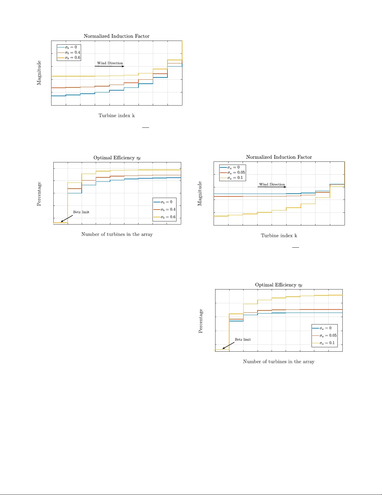
Stochastic Dynamic Programming for W ind Farm Po wer Maximization Y i Guo, Mario Rotea, T yler Summers Abstract — Wind plants can increase annual energy produc- tion with advanced control algorithms by coordinating the operating points of individual turbine contr ollers across the farm. It r emains a challenge to achieve perf ormance improve- ments in practice because of the difficulty of utilizing models that capture pertinent complex aerodynamic phenomena while remaining amenable to control design. W e f ormulate a multi- stage stochastic optimal control problem for wind farm power maximization and show that it can be solved analytically via dynamic programming . In particular , our model incor porates state- and input-dependent multiplicative noise whose distribu- tions capture stochastic wind fluctuations. The optimal control policies and value functions explicitly incorporate the moments of these distributions, establishing a connection between wind flow data and optimal feedback control. W e illustrate the results with numerical experiments. I . I N T RO D U C T I O N W ind ener gy is an important component of future energy systems to meet growing energy demands. As wind power continues to account for a larger portion of the world-wide energy portfolio, the optimal operation of wind farms of fers both challenges and opportunities to further improve perfor- mance at the levels of single turbines, wind farms, and power grids. Due to nonlinear aerodynamic interaction through wakes and unpredictable wind variations, future optimal control strategies for wind farms will require sophisticated models to capture and manage stochastic wind fluctuations. Maximizing the wind power capture has been discussed in the scope of wind turbines [1]–[4] and wind farms [5]– [26]. In Re gion 2 operation (belo w-rated wind speed), the wind plant is operated to maximize the power output. In this regime, there are inherent tradeoffs between the wake of upstream turbines and the power extracted from downstream turbines. Due to this aerodynamic coupling, maximizing total power of wind farms cannot be achiev ed by myopically max- imizing the power output for each individual wind turbine in the array [27]. Therefore, depending on layout and wind conditions, it may be essential to hav e a coordinated control framew ork for wind farms to determine the optimal control strategy for each wind turbine to improv e annual ener gy production. Many challenges and related solutions for wind farm power maximization ha ve been highlighted and discussed in [1]. Recent control strategies for optimal operation hav e This material is based on work supported by the National Science Foundation under grant CMMI-1728605. This project was partially funded by The Univ ersity of T exas at Dallas Office of Research through the SCI program. Y . Guo, M. Rotea and T . Summers are with the Department of Mechanical Engineering, The Uni versity of T exas at Dallas, Richardson, TX, 75080, USA, email: { yi.guo2, rotea, tyler .summers } @utdallas.edu. been proposed using both model-based [6]–[14], [19], [20], [22], and model-free strategies [17], [21], [24]–[26]. Model- based strategies provide solutions that typically have faster response times than model-free approaches. Ho we ver , the models used for control design can deviate from actual wind field and turbine characteristics in practice, which can limit the effecti veness of model-based control strategies. The reader is referred to the introduction in [17], and the references therein, for further discussion on model-based and model-free strategies for wind plant power maximization. In this paper , we focus on wind power maximization in Region 2. The work presented here generalizes the simple actuator disk model (ADM) utilized in [22] to a stochastic version and pose a multi-stage stochastic optimal control problem for wind farm power maximization. The stochastic actuator disk model balances complexity and tractability by incorporating unsteady aerodynamic phenomena into the distributions of random variables in the model. Estimates of the statistics of these distributions can then be exploited in the control algorithm to impro v e overall efficienc y of the farm in the presence of stochastic wind flow . Our main contributions are as follows: - W e formulate a multi-stage stochastic optimal control problem for wind f arm po wer maximization and show that it can be analytically solved via dynamic program- ming. In particular , our model generalizes that of [22] by incorporating state- and input-dependent multiplica- tiv e noises to capture the uncertain wake effects of wind turbines. The stochastic version of the ADM relaxes a strong assumption of a deterministic ADM, such as steady wind o ver the rotor disk. In contrast to existing work, the proposed stochastic multi-stage formulation allows us to maximize the wind farm power by ex- plicitly incorporating information about the probability distributions of wind fluctuations into control decisions. - By solving the proposed multi-stage stochastic opti- mization, we show that the optimal feedback control policies for the turbines are linear with respect to up- stream wind velocity , but in contrast to [22], the optimal gain coef ficients depend explicitly on the statistics of the multiplicativ e noises, which can be estimated from high- fidelity wind flow simulations or experimental data. This provides a direct connection between statistical properties of the unsteady wind flow physics and the optimal feedback control of wind farms. W e also show that for the stochastic ADM with both multiplicativ e and additiv e noise, the optimal policies are nonlinear . The framework, while elementary for real-world applica- tions, illustrates a rigorous process for incorporating flow statistics into the wind farm power maximization problem. The dependence of control solutions on the statistics of the wind fluctuations makes intuitive sense, as one cannot expect a single control algorithm to be optimal under a range of unsteady wind conditions. In future work, we will extend the stochastic approach presented in this paper to more representativ e, yet tractable, models of the flow physics and loads as done in [18]. I I . P RO B L E M F O R M U L AT I ON Our model is a generalization of the one in [22], which utilizes the actuator disk model (ADM) [28], [29]. Let P denote the power extracted by an ideal turbine rotor , let F denote the force done by the wind on the rotor , let V 0 denote the free stream upwind velocity , let V denote the wind velocity at the disk, and let V 1 denote the far wake velocity . The ADM model is then P = F V , (1a) F = ρA ( V 0 − V 1 ) V , (1b) V = V 0 − u, (1c) V 1 = V 0 − 2 u, (1d) where ρ is the air density , A is the rotor swept area, and u ≥ 0 is the reduction in air velocity between the free stream and the rotor plane, which can be interpreted as a control input. In practice, u can be controlled by adjusting the angular rotor speed or the collectiv e blade pitch angle. Fig. 1. A cascade of N wind turbines; k = 0 indicates the most upstream location. Deterministic Model: W e consider a one-dimensional cascade of wind turbines, illustrated in Fig. 1. W e assume that the wind direction is along the row of turbines and is not varying. The ADM model giv en in (1) can be written in state-space form by letting x k and x k +1 denote the wind velocity upstream and downstream of the k -th turbine (i.e., x k = V k in (1d), for k = 0 , 1 ). The scalar control input for the k -th turbine is denoted by u k , which is the controllable wind velocity deficit at the rotor disk, and y k is an output to estimate the power extraction of turbine k (i.e., y k = V k − u k in (1c)). Then the velocity V k +1 in the far wake of the rotor (1d) and the rotor ef fect at the disk in velocity (1c) can be written as below in (2a) and (2b). The power extraction of the k -th wind turbine using ADM model (1) in state-space expression is gi ven in (2c) x k +1 = x k − 2 u k , (2a) y k = x k − u k , (2b) p k ( y k , u k ) = 2 ρAy 2 k u k , (2c) where the control input is constrained by u k ∈ [0 , 1 2 x k ] so that the wind velocity in the far wake remains positi ve. T o simplify the notation, we eliminate the constant in (2c) and come to the constant-free turbine po wer function ` ( x k , u k ) , which will serve as a stage cost in our subsequent multi-stage optimal control problem ` ( x k , u k ) = ( x k − u k ) 2 u k . (3) Note that this function is jointly cubic in the state and control input. Further details of this model may be found in [22]. Stochastic Model: The simple model described above captures basic wind farm turbine interactions. But it fails to capture stochastic wind fluctuations that are also relev ant to optimizing the total po wer output. High fidelity computa- tional fluid dynamic models offer extreme detail of flows but are cumbersome to incorporate into high-le vel operational decision making. Therefore, we consider here a stochastic extension of the deterministic actuator disk model abov e that can capture more complex phenomena, such as stochastic wind fluctuations, while remaining computationally tractable. Fig. 2. Stochastic actuator disk model and stream-tube diagram for wind power extraction. The solid and dashed lines indicate the wind field mean and associated stochastic variations, respectively , which relate to the moments of the multiplicative variations parameters a k and b k . The stochastic actuator disk model is gi ven by x k +1 = a k x k + b k u k , (5) where a k ∼ P a,k is a state multiplicativ e random v ariable and b k ∼ P b,k is an input multiplicativ e random variable. The model is illustrated in Fig. 2. W e assume that the random variables a k and b k are independent for all k and independent of each other . This model captures stochastic wind fluctuations. In particular , the multiplicative noises a k and b k provide a simple model for the inherent stochasticity of far wake recovery . W e assume that moments up to order three of each of the distrib utions P a,k , P b,k are kno wn (or can be estimated from high-fidelity simulation or experimental data). For the state mean dynamics to match the deterministic model (2a), we can set E [ a k ] = 1 , E [ b k ] = − 2 . ψ k = − 3 Q k +1 Σ b,k µ a,k − 2 + p (3 Q k +1 Σ b,k µ a,k − 2) 2 − 3( Q k +1 Γ b,k + 1)(3 Q k +1 Σ a,k µ b,k + 1) 3( Q k +1 Γ b,k + 1) , (4a) Q k = (1 − ψ k ) 2 ψ k + Q k +1  Γ a,k + Γ b,k ψ 3 k + 3Σ b,k µ a,k ψ 2 k + 3Σ a,k µ b,k ψ k  . (4b) I I I . S T OC H A S T I C O P T I M A L C O N T R O L F O R W I N D P O W E R M A X I M I Z A T I O N The objective of the operator is to select control inputs u 0 , ..., u N − 1 to maximize the aggregate po wer of the wind turbine cascade giv en by the sum of (3) ov er all turbines. Howe ver , since in the stochastic model the states (and there- fore the power outputs) are random variables, we maximize the expected aggregate power and search for closed-loop feedback control policies that specify control inputs as a function of the state x k . In particular, we seek to solve the multi-stage stochastic optimal control problem max π 0 ,...,π N − 1 E N − 1 X k =0 ( x k − u k ) 2 u k , (6) where the decision variables π k ( · ) are the control policies (i.e., u k = π k ( x k ) ), and the expectation is taken with respect to the random variable sequences a k , b k . As in [22], we will show that the optimal policies are linear and the optimal value functions are cubic . In contrast to [22], the parameters of both the optimal policies and value functions depend on the moments of the distribution of the random variables in the model. W e have the follo wing main result. Theor em 1: Consider the wind farm power maximization problem for a cascade of N identical turbines modeled with the stochastic actuator disk model (5), (6). Let x 0 denote the free stream velocity entering the cascade. The distributions of a k and b k are described by their raw moments up to third order , namely their means µ a,k , µ b,k , second (raw) moments Σ a,k , Σ b,k and third (raw) moments Γ a,k , Γ b,k . Under these assumptions, the optimal feedback control policies are linear in the state and given by u ∗ k = π ∗ ( x k ) = ψ k x k , k = 1 , ..., N − 1 , (7) where the gain coefficients ψ k are giv en in (4a) and the back- wards recursion (4b) for k = N − 1 , ..., 0 with initialization Q N = 0 . The maximum po wer produced by the wind f arm as a function of initial upstream wind velocity is giv en by P ∗ 0 ( x 0 ) = 2 ρAQ 0 x 3 0 , (8) where ρ is the air density , A is the rotor swept area, and Q 0 is the initial value of the backwards recursion (4b) with Q N = 0 . Pr oof: The dynamic programming algorithm [30], [31] for solving stochastic optimal control problems is gi ven by the recursion G ∗ k ( x k ) = max u k ∈ [0 , 1 2 x k ] E  ` ( x k , u k ) + G ∗ k +1 ( x k +1 ))  , π ∗ ( x k ) = arg max u k ∈ [0 , 1 2 x k ] E  ` ( x k , u k ) + G ∗ k +1 ( x k +1 ))  , (9) where G ∗ k ( x k ) represents the optimal (normalized) wind farm power from turbine k as a function of the state x k , with initialization G ∗ N ( x k ) = 0 . W e first solve the last tail sub- problem at k = N − 1 with G ∗ N ( x ) = 0 . W e have ∂ ` ( x N − 1 , u N − 1 ) ∂ u N − 1 = ( x N − 1 − u N 1 )( x N − 1 − 3 u N − 1 ) = 0 , for which the policy u ∗ N − 1 = 1 3 x N − 1 is the unique maxi- mizer and satisfies the constraint u N − 1 ∈ [0 , 1 2 x N − 1 ] . Sub- stituting this optimal policy back into the value expression yields the optimal power function G ∗ N − 1 ( x N − 1 ) = 4 27 x 3 N − 1 . Note that this function is a cubic in the state. Accordingly , we parameterize the optimal po wer functions as G ∗ k ( x k ) = Q k x 3 k and consider a general step in the backward recursion. T o obtain the optimal policy , we define the function inside the maximization operation G k ( x k , u k ) := ( x k − u k ) 2 u k + Q k +1 E  ( a k x k + b k u k ) 3  . (10) Expanding the second term and taking the expectation by utilizing the (raw) moment information from the distrib utions of a k and b k , and then taking the partial deriv ative of G k ( x k , u k ) with respect to u k giv es a quadratic polynomial in u k . As above, one of the roots of this polynomial cor- responds to the unique maximizing input, which is a linear function of the state. Carrying out the algebra yields u ∗ k = π ∗ ( x k ) = ψ k x k , (11) where the gain parameters ψ k are given in (4a). Note that the optimal policies all satisfy the constraints on u k . T o obtain a backwards recursion for the value function coef ficients Q k , we substitute u ∗ k = ψ k x k back into (10) G ∗ k ( x k , u ∗ k ) = Q k x 3 k =( x k − u ∗ k ) 2 u ∗ k + Q k +1 E  ( a k x k + b k u ∗ k ) 3  . (12) Since u ∗ k is linear in x k , the optimal v alue functions are cubic in the state. Matching the coef ficients on both sides of (12), we come to (4b). Eq. (8) follows from (12) for k = 0 , (6) and (2c), which concludes the proof. Remark 1: (Optimal policies and value functions with central moments.) The random v ariables a k and b k can also be described by their higher-order central moments, namely their variances σ 2 a,k , σ 2 b,k and ske wnesses γ a,k , γ b,k . The optimal linear state feedback control policies can also be written in terms of central moments instead of raw moments by using Σ = σ 2 + µ 2 , Γ = σ 3 γ + 3 σ 2 µ + µ 3 . (14) π ∗ N − 2 ( x ) = − ∆ k + q ∆ 2 N − 2 − 3( Q N − 1 Γ b,N − 2 + 1)  (3 Q N − 1 Σ a,N − 2 µ b,N − 2 + 1) x 2 + 3 Q N − 1 Σ c,N − 2 µ b,N − 2  3( Q N − 1 Γ b,N − 2 + 1) , where, ∆ N − 2 = (3 Q N − 1 Σ b,N − 2 µ a,N − 2 − 2) x. (13) Cor ollary 1: Under the assumptions of Theorem 1, we define the efficienc y η ` of the ` -th sub-array 1 by η ` := E  P ` 1 2 ρAx 3 `  , (15) where x ` is the free stream velocity entering the subarray cascaded turbines from ` to N − 1 and P ` denotes the aggregated power from the ` -th subarray of wind turbines. The optimal efficienc y η ∗ ` of the l -th sub-array has the form η ∗ ` = 4 Q ` , ∀ ` ∈ { 0 , . . . , N − 1 } , (16) which is achiev ed with the optimal control sequence u ∗ ` , . . . , u ∗ N − 1 , where Q ` is calculated from (4b). Pr oof: The maximum power produced by the N − ` turbines is P ∗ ` = 2 ρAQ ` x 3 ` , (17) under the optimal control sequence u ∗ ` , . . . , u ∗ N − 1 with Q ` computed via (4b). W e substitute the optimal power (17) into (15) and obtain (16), which concludes the proof. Next, we consider a stochastic actuator disk model with both multiplicati ve and additive noise, which allows a more general description of uncertainty in wind fluctuations. In- terestingly , in contrast to classical linear quadratic problems, when additi v e noise is included the optimal policies are no longer linear in general, and so the optimal v alue functions are no longer cubic. This highlights a computational limita- tion with this more general model that mak es the approach more difficult to implement in practice. Theor em 2: (Stochastic actuator disk model with additive noise.) Consider the stochastic ADM (5) with additive noise x k +1 = a k x k + b k u k + c k , (18) where c k ∼ P c is a zero-mean additiv e random variable with second moment Σ c,k and third moment Γ c,k . In the penultimate tail subproblem, the optimal policy has the nonlinear form π ∗ N − 2 ( x ) = δ x + p α + β x 2 for some constants δ , α , and β ; the exact expression is giv en in (13). As a result, the corresponding optimal value function at turbine location N − 2 is non-cubic, and so the remaining optimal policies and value functions are nonlinear and non- cubic, respectiv ely . Pr oof: Consider again the dynamic programming re- cursion (9). Since G ∗ N ( x ) = 0 , the last tail subproblem is 1 The efficiency η ` defined here quantifies the energy extraction of sub- array ` compared to energy in the wind entering the sub-array . Note that due to aerodynamic wake coupling, it is possible for the optimal efficiency of the sub-array to exceed the efficienc y obtained by independently setting individual turbine induction factors to achie ve the single-turbine Betz limits. identical to that in Theorem 1, so that G ∗ N − 1 ( x N − 1 ) = 4 27 x 3 N − 1 . Consider no w the penultimate tail subproblem for k = N − 2 G N − 2 ( x, u ) = ( x − u ) 2 u + 4 27 E  ( a k x + b k u + c k ) 3  . (19) T aking the expectation of the second term by utilizing the (raw) moments of a k , b k and c k , and then taking the partial deriv ative with respect to u and setting to zero yields a quadratic optimality condition in u . Carrying out some algebra as above, it turns out that the roots of this polynomial are no longer linear in the state, in contrast to the results in Theorem 1. The optimal control policy is thus a nonlinear function of state of the form π ∗ N − 2 ( x ) = δ x + p α + β x 2 for some constants δ , α , and β . The exact expression for the maximizing control input derived from the quadratic optimality condition is given in (13). It can also be seen that when the additive noise variance Σ c,k is zero (i.e., the additiv e noise is absent since it also has zero mean), then α = 0 and we recover the linear policy of of Theorem 1 since x ≥ 0 . Finally , these observations also lead to the conclusion that none of the remaining optimal policies and value functions are linear and cubic, respectively , and will in fact become increasingly complicated as the recursion proceeds backward to ward the beginning of the array . I V . N U M E R I C A L E X P E R I M E N T S T o illustrate our results, we consider a cascade with N = 10 identical turbines to analyze the performance of the optimal gain sequence { ψ 0 , . . . , ψ 9 } for the proposed stochastic actuator disk model. As is commonly done in the literature [28], [29], we refer to these gains as induction factors . The stochastic model parameters a k and b k are all independent of each other and spatially homogeneous ( µ a,k = µ a , µ b,k = µ b , σ a,k = σ a , σ b,k = σ b , γ a,k = γ a and γ b,k = γ b , ∀ k ) 2 . Fig. 3 illustrates the optimal induction factor sequence { ψ 0 , . . . , ψ 9 } and Fig. 4 depicts the optimal efficiency η ∗ ` un- der dif ferent standard de viation values of the input-dependent multiplicativ e noise b k . The induction factors in Fig. 3 are normalized by 1 / 3 , which is the value achieving the Betz limit for a single isolated turbine [28]. W e set the mean value µ a to 1, and the ske wness to zero. Fig. 4 demonstrates that the optimal array efficiency improv es with increasing variance on b k . This result is intuiti vely reasonable, in the sense that higher variability of the velocity deficits in the far wake may lead to increased po wer e xtraction. W e speculate that this multiplicative stochastic perturbation on the velocity 2 T o have clearer interpretation of our results, we discuss the results in the terms of central moments. No additive noise is considered in this section. 0 1 2 3 4 5 6 7 8 9 0 0.2 0.4 0.6 0.8 1 Fig. 3. Normalized induction factors defined as ψ k 1 / 3 for deterministic model ( µ a = 1 , µ b = − 2 ) and stochastic model with various v alues of input-dependent multiplicativ e noise standard deviation ( µ a = 1 , σ a = 0 , µ b = − 2 , σ b > 0 , γ a = 0 and γ b = 0 ). 1 2 3 4 5 6 7 8 9 10 0.6 0.62 0.64 0.66 0.68 Fig. 4. Comparison of optimal efficiency η ` for deterministic model ( µ a = 1 , µ b = − 2 ) and stochastic model with various values of input-dependent multiplicativ e noise standard deviation ( µ a = 1 , σ a = 0 , µ b = − 2 , σ b > 0 , γ a = 0 and γ b = 0 ). deficit may provide a mathematically simple way of cap- turing physical phenomena such as mixing or entrainment, which are known to promote energy extraction [32], [33] Note also that the case σ b = 0 reproduces the results for the deterministic ADM model in [22]. It should be noted that as the standard de viation σ b is increased, the induction factors increase. That is, the leading upstream turbines are working more as the multiplicative noise is increased; which again is consistent with the conv entional wisdom that the more turbulent the wind is the closer the turbines should be to their isolated optimum set point [34] Figures 5 and 6 provide the optimal induction factor sequence and efficienc y under different standard deviation values of the state-dependent noise on a k , and without input-dependent noise (i.e., b k is fixed and constant for all k ). Both figures demonstrate that the optimal induction factor sequence from the stochastic actuator disk model also increases the efficiency and improv es performance under larger variations. T o match the expected wind velocity of the con ventional deterministic ADM, the mean value of the state-dependent noise should be set to unity (i.e., µ a = 1 ) [22]. Howe v er , having µ a = 1 together with a non-zero variance in the state-dependent multiplicativ e noise a k leads to null optimal induction factors for leading upstream turbines, since in this case the model essentially predicts that additional energy will be injected into the wake further downstream. This indicates that the parameters in the stochastic ADM should be carefully calibrated based on measured data in order to capture appropriate (possibly heterogeneous) spatio-temporal flow variations and obtain reasonable control policies for the array . T o appropriately incorporate stochasticity of the wind flow , we set the mean value of a k to µ a = 0 . 99 , and vary the standard de viation σ a to describe statistical fluctuations. The key observation is that regardless of the v alue of µ a , the proposed approach improves efficienc y with increasing variance by exploiting statistical knowledge of wind field fluctuations and incorporating this information into optimal control policies for wind farm power maximization. 0 1 2 3 4 5 6 7 8 9 0 0.2 0.4 0.6 0.8 1 Fig. 5. Normalized induction factor defined as ψ k 1 / 3 for deterministic model ( µ a = 0 . 99 , µ b = − 2 ) and for stochastic model with various values of state-dependent multiplicative noise standard deviation ( µ a = 0 . 99 , σ a > 0 , µ b = − 2 , σ b = 0 , γ a = 0 and γ b = 0 ). 1 2 3 4 5 6 7 8 9 10 0.6 0.62 0.64 0.66 0.68 Fig. 6. Comparison of optimal efficienc y η ` for deterministic model ( µ a = 0 . 99 , µ b = − 2 ) and stochastic model with various values of state-dependent multiplicative noise standard deviation ( µ a = 0 . 99 , σ a > 0 , µ b = − 2 , σ b = 0 , γ a = 0 and γ b = 0 ). The stochastic actuator disk model of a wind farm with cascaded wind turbines captures stochastic wind fluctua- tions. By definition, the optimal control laws derived from stochastic dynamic programming achiev e superior perfor- mance to laws deriv ed from a deterministic model of the same comple xity , allowing the turbines to recognize and react to the particular wind field characteristics. Data derived di- rectly from measurements or simulations can be incorporated directly into the control law to improve the aerodynamic efficienc y a wind farm for specific wind fluctuation statistics. It is worth emphasizing that more work is necessary to incorporate tractable noise models that are consistent with the flo w physics; this conference paper is a first step in this direction. V . C O N C L U S I O N S A N D O U T L O O K S W e ha ve formulated a multi-stage stochastic optimal con- trol problem for maximizing the power output of a one dimensional wind farm array and shown that it can be solved analytically via dynamic programming. The optimal control policies depend explicitly on the statistics of multiplicati ve noise, which can be related to stochastic wind fluctuations. Our results provide an initial step toward defining a wind farm control strategy that tractably incorporates statistical knowledge of stochastic wind fluctuations. Howe ver , there remain sev eral lines of future work that can extend the present results in various ways to more fully understand the possibilities and limits for maximizing annual energy production. Our future work will in volv e (a) utilizing more realistic wake models; (b) estimating necessary statistics from high-fidelity numer- ical simulations and experimental data; (c) performance ev aluation of the policies on high-fidelity models, which may improve the results in [33]; (d) considering more realistic array geometries; (e) exploring computationally efficient approximation of nonlinear optimal control strategies; if needed. R E F E R E N C E S [1] L. Y . Pao and K. E. Johnson, “ A tutorial on the dynamics and control of wind turbines and wind farms, ” in American Control Conference , pp. 2076–2089, June 2009. [2] Y . Xiao, Y . Li, and M. A. Rotea, “CAR T3 field tests for wind turbine region-2 operation with extremum seeking controllers, ” IEEE T ransactions on Control Systems T echnology , vol. 27, no. 4, pp. 1744– 1752, 2019. [3] L. Y . Pao and K. E. Johnson, “Control of wind turbines, ” IEEE Contr ol Systems Magazine , vol. 31, no. 2, pp. 44–62, 2011. [4] I. Munteanu, A. I. Bratcu, N.-A. Cutululis, and E. Ceanga, Opti- mal Contr ol of Wind Energy systems: T owar ds a Global Appr oach . Springer Science & Business Media, 2008. [5] J. Schepers and S. V an der Pijl, “Impro ved modelling of wake aerody- namics and assessment of new farm control strategies, ” in Journal of Physics: Conference Series , v ol. 75, p. 012039, IOP Publishing, 2007. [6] K. E. Johnson and N. Thomas, “Wind farm control: Addressing the aerodynamic interaction among wind turbines, ” in American Control Confer ence , pp. 2104–2109, June 2009. [7] T . Knudsen, T . Bak, and M. Soltani, “Distributed control of large- scale offshore wind farms, ” in European W ind Ener gy Confer ence and Exhibition , Citeseer, 2009. [8] V . Spudic, M. Jelavic, M. Baotic, and N. Peric, “Hierarchical wind farm control for power/load optimization, ” The Science of Making T orque fr om W ind , 2010. [9] D. Madjidian, K. M ˚ artensson, and A. Rantzer , “ A distributed power coordination scheme for fatigue load reduction in wind farms, ” in American Control Confer ence , pp. 5219–5224, June 2011. [10] M. Soleimanzadeh and R. Wisnie wski, “Controller design for a wind farm, considering both po wer and load aspects, ” Mechatr onics , vol. 21, no. 4, pp. 720–727, 2011. [11] M. Kristalny and D. Madjidian, “Decentralized feedforward control of wind farms: prospects and open problems, ” in IEEE Conference on Decision and Contr ol and European Control Confer ence , pp. 3464– 3469, Dec. 2011. [12] T . Horvat, V . Spudi ´ c, and M. Baoti ´ c, “Quasi-stationary optimal control for wind farm with closely spaced turbines, ” in IEEE International Con vention MIPRO , pp. 829–834, July 2012. [13] B. Biegel, D. Madjidian, V . Spudi ´ c, A. Rantzer, and J. Stoustrup, “Distributed lo w-complexity controller for wind power plant in derated operation, ” in IEEE International Conference on Control Applications , pp. 146–151, Aug. 2013. [14] E. Bitar and P . Seiler , “Coordinated control of a wind turbine array for power maximization, ” in American Contr ol Conference , pp. 2898– 2904, June 2013. [15] L. Buccafusca and C. L. Beck, “Maximizing power in wind turbine arrays with v ariable wind dynamics, ” in IEEE Conference on Decision and Control , pp. 2667–2672, Dec. 2018. [16] L. Buccafusca, C. Beck, and G. Dullerud, “Modeling and maximizing power in wind turbine arrays, ” in IEEE Conference on Control T echnology and Applications , pp. 773–778, Aug. 2017. [17] U. Ciri, M. A. Rotea, and S. Leonardi, “Model-free control of wind farms: A comparati ve study between individual and coordinated extremum seeking, ” Renewable ener gy , v ol. 113, pp. 1033–1045, 2017. [18] V . Santhanagopalan, M. Rotea, and G. Iungo, “Performance optimiza- tion of a wind turbine column for different incoming wind turbulence, ” Renewable Energy , vol. 116, pp. 232–243, 2018. [19] P . Gebraad, F . T eeuwisse, J. V an Wingerden, P . A. Fleming, S. Ruben, J. Marden, and L. Pao, “Wind plant power optimization through yaw control using a parametric model for wake effectsa CFD simulation study , ” W ind Energy , vol. 19, no. 1, pp. 95–114, 2016. [20] J. P . Goit and J. Meyers, “Optimal control of ener gy e xtraction in wind-farm boundary layers, ” J ournal of Fluid Mechanics , vol. 768, pp. 5–50, 2015. [21] P . Gebraad and J. V an W ingerden, “Maximum power -point tracking control for wind farms, ” W ind Ener gy , vol. 18, no. 3, pp. 429–447, 2015. [22] M. A. Rotea, “Dynamic programming framework for wind power maximization, ” IF AC Pr oceedings V olumes , vol. 47, no. 3, pp. 3639– 3644, 2014. [23] K. E. Johnson and G. Fritsch, “ Assessment of extremum seeking control for wind farm energy production, ” W ind Engineering , v ol. 36, no. 6, pp. 701–715, 2012. [24] Z. Y ang, Y . Li, and J. E. Seem, “Maximizing wind farm ener gy capture via nested-loop e xtremum seeking control, ” in ASME Dynamic Systems and Control Confer ence , pp. 1–8, Oct. 2013. [25] J. R. Marden, S. D. Ruben, and L. Y . Pao, “ A model-free approach to wind farm control using game theoretic methods, ” IEEE T ransactions on Contr ol Systems T echnology , vol. 21, no. 4, pp. 1207–1214, 2013. [26] J. Park, S. Kwon, and K. H. Law , “Wind farm power maximization based on a cooperati ve static game approach, ” in 2013 Active and P as- sive Smart Structures and Inte grated Systems , vol. 8688, p. 86880R, April 2013. [27] M. Steinbuch, W . De Boer, O. Bosgra, S. Peeters, and J. Ploeg, “Optimal control of wind power plants, ” J ournal of W ind Engineering and Industrial Aerodynamics , vol. 27, no. 1-3, pp. 237–246, 1988. [28] T . Burton, D. Sharpe, and N. Jenkins, Handbook of W ind Energy . John W iley & Sons, 2001. [29] J. F . Manwell, J. G. McGowan, and A. L. Rogers, W ind Energy Explained: Theory , Design and Application . John W iley & Sons, 2010. [30] R. Bellman, “The Theory of Dynamic Programming, ” tech. rep., RAND Corp Santa Monica CA, 1954. [31] D. P . Bertsekas, D. P . Bertsekas, D. P . Bertsekas, and D. P . Bertsekas, Dynamic Progr amming and Optimal Contr ol , vol. 1. Athena scientific Belmont, MA, 2005. [32] C. V erHulst and C. Meneveau, “Large eddy simulation study of the kinetic energy entrainment by ener getic turbulent flow structures in large wind farms, ” Physics of Fluids , vol. 26, no. 2, p. 025113, 2014. [33] C. Santoni, U. Ciri, M. Rotea, and S. Leonardi, “Development of a high fidelity CFD code for wind farm control, ” in American Contr ol Confer ence , 2015. [34] U. Ciri, M. Rotea, C. Santoni, and S. Leonardi, “Large-eddy simula- tions with extremum-seeking control for individual wind turbine power optimization, ” W ind Energy , vol. 20, no. 9, pp. 1617–1634, 2017.