Linear robust adaptive model predictive control: Computational complexity and conservatism -- extended version

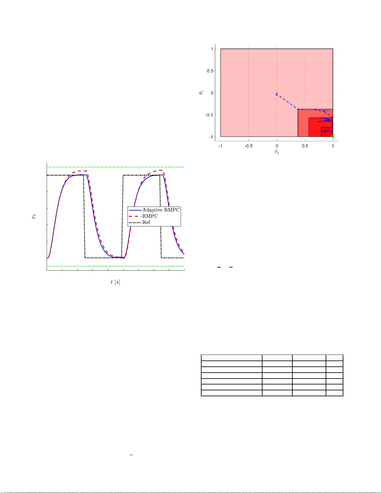
1 Linear rob ust adapti v e model predicti v e con trol: Computational comple xity and conserv atism - e xtended version Johann es K ¨ ohler 1 , Elisa And ina 2 , Raff aele Soloperto 1 , Matthias A. M ¨ uller 3 , Frank Allg ¨ ower 1 Abstract —In this paper , we present a robust adaptive model predictiv e control (M P C) sch eme f or linear system s sub ject to parametric uncertainty and additive disturbances. The proposed approach prov ides a computationally efficient formulation with theoretical guarantees (constraint satisfaction and stability), while allowing fo r reduced conserv atism an d improv ed p erformance due t o onli ne parameter adaptation. A mo ving wind ow parameter set identi fication is used to comput e a fixed complexity parameter set b ased on past data. Robust constraint satisfaction is achieved by using a compu t ationally efficient tube b ased robust M PC method. The p redicted cost function i s based on a least mean squares point estima te, wh ich ensure s finite-gain L 2 stability of the closed loop. T he ov erall algorithm has a fixed ( u ser specified) computational complexity . W e i l lustrate the applicabilit y of the approach and the trade-off b etween conservatism and computa- tional complexity using a numerical example. This paper is an ex tended version of [1], and contains additional details regarding t h e theoretical proof of Th eorem 1 , the nu merical example (Sec. IV), and the offline computations in Appendix A–B. I . I N T RO D U C T I O N Motivation: Mo del pred ictiv e co ntrol (MPC) [2], [3] is an optimization based control metho d that can handle complex multi-inpu t multi-outp ut (MI MO) systems with har d state and input constraints. Model uncertainty and disturbances ca n have an adversarial impact o n perf ormance a nd co n straint satisfaction. T hese issues can b e a ddressed using r obust MPC formu latio ns, which can, howe ver , be q u ite conser vati ve in case of parametric u ncertainty . This motiv ates the d esign of adaptive/learning MPC schemes that can use o nline model adaptation to red uce the con servatism an d improve the per- forman ce. In this pap e r , we p rovide a r obust adap ti ve MPC formu latio n that provides theoretical guaran tees, allows for online perfo rmance improvement an d is compu tationally e f- ficient. This wo rk was supported by the G erman Researc h Foun dation under Grants GRK 2198/1 - 277536708, AL 316/12- 2, and MU 3929/ 1-2 - 279734922. The authors thank the Internati onal Max Planck Research S chool for Intell igent Systems (IMPRS-IS) for supporting Raff aele Soloperto. 1 Johannes K ¨ ohler , Raf fael e Solopert o and Frank Allg ¨ ower are with the Institut e for Systems Theory and Automat ic Control , Uni versity of Stuttga rt, 70550 Stuttgart, Germany . (email: { johannes.koe hler, raf- fae le.soloperto, frank.allgo wer } @ist.uni-stut tgart.de). 2 Elisa Andina is a M.Sc. stude nt at th e Uni versit ` a di Bol ogna, 40136 Bologna , Itali y (email: elisa.andina@st udio.unibo.it). 3 Matthi as A. M ¨ uller is with the Institute of Automatic Control, Leibniz Uni versity Hannov er , 30167 Hanno ver , Germany . (email:muell er@irt.uni- hanno ver .de). Related work: T u be based r obust MPC meth ods are the simplest way to en sure stability an d robust constraint sat- isfaction u nder uncertainty . Robust constraint satisfaction is typically achieved by including a pre -stabilizing feedback and computin g a polytop ic tub e that bo unds the unce r tain predicted trajectories, compare for example [4], [ 5], [6]. The perfor- mance and conser vatism of these ro bust MPC appr oaches can be improved b y using on line system identification or pa rameter adaptation . In [7], [8], a fixed un certainty descr ip tion is u sed to ensure robust constrain t satisfaction, while an onlin e adap ted mod el is used in the c o st functio n to improve p erforma n ce. The conservatism of the r obust MPC constrain t tighten ing can be red uced by using on line set-mem bership system iden- tification. For FIR systems, this has been propo sed in [9] and extended to time-varying systems an d stochastic uncertainty in [10] and [11], r e sp ectiv ely . In [12], this approach has been extended to g e neral lin ear state space mo dels, by combining set-membersh ip e stimation with th e hom othetic tube b ased robust MPC formulation in [6]. By using an additional least mean sq u are (L MS) poin t estimate f o r the cost function, this scheme also e n sures finite-gain L 2 -stability . The m ain drawback of this approach is that the resulting q uadratic progr am (QP) has significantly mor e optimization variables and co nstraints com pared to a n o minal MPC. Robust adapti ve MPC methods f or nonlinear systems can be foun d in [13]. Method s to explicitly incentivize or enforce learning o f the unkn own parameter s can be found in [14], [15], [16], [1 7], which is, however , not the g oal of this p aper . Contribution: In this work, we present a computationally efficient robust adap ti ve MPC scheme f or linear uncertain systems. Similar to [ 12], the pro posed method uses a set- membersh ip estimate for th e par ametric uncertain ty , a robust constraint tightening , and a cost fun ction based on a LM S point estimate. Correspondin gly , the proposed ro bust adaptive MPC sch e me shar es th e theo retical pr operties of the schem e in [1 2], i.e., e n sures ro bust constrain t satisfaction and finite- gain L 2 stability w .r .t. additive disturb ances. Compared to [12], we employ a m oving window set-member ship estimation to compute a hy percub e that boun ds the par ametric uncertain ty . Furthermo re, we use a rob ust constraint tightening based on the novel robust M PC framework in [ 5]. As a result, the propo sed robust adaptive MPC scheme has a fixed com- putationally complexity , which is only m oderately increased c  2019 IEEE. Personal use of this material is pe rmitted. Permission from IEEE m ust be obtained for all other uses, in any current or future media , includi ng reprint ing/republi shing this mater ial for advertising or promotional purpose s, creating ne w colle ctiv e works, for resale or redist ribution to s ervers or lists, or reuse of any copyri ghted compone nt of this work in other works. 2 compare d to a nominal MPC scheme. The m ain theo r eti- cal contribution o f this paper is to extend the robust MPC method presen te d in [5] to allow f or an online adaptation of the parametric uncertainty , while preserv ing th e theoretical proper ties and comp utational efficiency . Compared to [12], the propo sed appro ach can be more conservati ve. On the other hand, it h as a strongly red u ced co mputation al complexity . The trade off between compu tational comp lexity an d con- servatism in d ifferent ro bust MPC ap proach e s is discussed in detail and is quantitati vely in vestigated using a n u merical example. Th e n umerical example demo nstrates the b enefits of the propo sed adaptiv e formulation compared to a ro bust formu latio n. Furthermor e, the computatio nal ef ficiency of the propo sed formu lation in comparison to [12] is substantiated. After submission of this manu scr ipt, a co mpeting ap proach for robust adap tiv e MPC has bee n presented in [ 1 8] b ased on the robust approa ch in [4]. In terms of compu tational complexity and conservatism, the appro ach in [18] is located between the proposed ap proach an d the ap proach in [1 2], which is demonstra te d in the numer ical comparison . Outline: Section II presents the pr oblem setup and discusses the par ameter estimation. Section II I presents the proposed robust adap ti ve MPC scheme with c o rrespon ding theoreti- cal guarantees and a discussion regar d ing alternative rob ust MPC appro aches. Section IV demon strates the bene fits of the propo sed formu lation with a n umerical examp le. Section V conclud e s the pap er . The App e ndix contains ad ditional details. The results in this paper ar e based on th e thesis [ 19]. This paper is an extended version of the co nference pape r [1], containing detailed pr oofs and additional resu lts. Notation: The quad r atic norm with respect to a positive definite matrix Q = Q ⊤ is denoted by k x k 2 Q = x ⊤ Qx . Denote the unit hy p ercube by B p := { θ ∈ R p | k θ k ∞ ≤ 0 . 5 } . I I . P RO B L E M S E T U P A N D P A R A M E T E R E S T I M A T I O N This section in troduces the p roblem setup (Sec. II- A), the computatio n of set-membe r ship estimates (Sec . II-B) an d point estimates (Sec . II-C) for un known c o nstant pa r ameters. A. Setup W e co nsider a discrete-time linear system x t +1 = A θ x t + B θ u t + d t , (1) with state x t ∈ R n , input u t ∈ R m , additive disturban ces d t ∈ R n and u nknown b ut constant p a rameters θ = θ ∗ ∈ R p . Assumption 1. The disturban ce satisfies d t ∈ D for all t ≥ 0 , with D = { d ∈ R n | H d d ≤ h d } co mpact. The system ma trices depend a ffinely on the parameters θ ∈ R p A θ = A 0 + p X i =1 [ θ ] i A i , B θ = B 0 + p X i =1 [ θ ] i B i . Ther e exists a known prior parameter set Θ H C 0 := θ 0 ⊕ η 0 B p , η 0 ≥ 0 that co ntains the parameters θ ∗ . These con ditions are rather standa r d in the context of linear uncertain systems. For simplicity , we consider Θ H C 0 to be a hypercub e, however , any po lytope of fixed shape can be emp loyed . Extension s to time-v ary ing param eters are discussed in Section II I-D. W e con sider mixed constraints on the state and in put ( x t , u t ) ∈ Z , ∀ t ≥ 0 , (2) with the comp act polytope Z = { ( x, u ) ∈ R n + m | F j x + G j u ≤ 1 , j = 1 , . . . , q } . The co ntrol goa l is to stabilize the origin , while satisfying the constraints (2) despite the d istur bances d t and the uncertainty in the param eters θ . B. Set membership estimation In o rder to satisfy the constraints (2), the uncertainty in the parameters θ needs to be taken into account, which in turn may lead to conservatism. T o reduce this co nservatism, a set membersh ip estimation algorithm is u sed to co mpute a smaller set Θ H C t ⊆ Θ H C 0 that contain s the true para m eters θ ∗ , as done in [9] , [12], [18]. Define D ( x, u ) := [ A 1 x + B 1 u, . . . , A p x + B p u ] ∈ R n × p . Giv en ( x t − 1 , u t − 1 , x t ) , the n on falsified parameter set is g i ven by the polyto p e ∆ t := { θ ∈ R p | x t − A θ x t − 1 − B θ u t − 1 ∈ D } . The following algor ith m uses a gi ven hypercub e Θ H C t − 1 and the past M ∈ N sets ∆ t − k in a movin g window fashion to compute a tighter non falsified h ypercub e Θ H C t using linear progr amming (LP). Algorithm 1 Moving window hyp ercube update Input: { ∆ k } k = t,...,t − M − 1 , Θ H C t − 1 . Ou tput: Θ H C t = θ t ⊕ η t B p Define po lytope Θ M t := Θ H C t − 1 T t k = t − M − 1 ∆ k . Solve 2 p L Ps ( i = 1 , . . . , p ) : θ i,t, min := min θ ∈ Θ M t e ⊤ i θ , θ i,t, max := max θ ∈ Θ M t e ⊤ i θ , with u nit vector e i = [0 , . . . , 1 , . . . , 0] ∈ R p , [ e i ] i = 1 . Set [ θ t ] i = 0 . 5 ( θ i,t, min + θ i,t, max ) . Set η t = max i ( θ i,t, max − θ i,t, min ) . Project: θ t on θ t − 1 ⊕ ( η t − 1 − η t ) B p . Lemma 1. Let Assumption 1 hold . F or t ≥ 0 the r ecu rsively updated sets Θ H C t , Θ M t contain the tr ue parameters θ ∗ and satisfy Θ M t ⊆ Θ H C t ⊆ Θ H C t − 1 . Pr oof. W e define the unique tig h t hyperb ox overapproxim a- tion o f Θ M t as Θ H B t = { θ ∈ R p | [ θ ] i ∈ [ θ i,t, min , θ i,t, max ] } , which satisfies Θ M t ⊆ Θ H B t . Giv en that by d e finition Θ M t ⊆ Θ H C t − 1 and the set Θ H B t is the u n ique tight hyper box over- approx imation of Θ M t , we have Θ H B t ⊆ Θ H C t − 1 and thus η t − 1 ≥ η t . Part I. Th e proje c tio n ensures Θ H C t = θ t ⊕ η t B p ⊆ θ t − 1 ⊕ ( η t − 1 − η t ) B p ⊕ η t B p = Θ H C t − 1 . 3 Part II. In the following, we show Θ H C t ⊇ Θ H B t ⊇ Θ M t . Th is claim reduc e s to [ θ i,t, min , θ i,t, max ] ⊆ [ θ ] i ⊕ η t [ − 0 . 5 , 0 . 5] . W ith - out lo ss of generality , we only sh ow θ i,t, min ≥ [ θ ] i − 0 . 5 η t , the case θ i,t, max ≤ [ θ ] i + 0 . 5 η t is analo gous. Case (i): Suppose 0 . 5 ( θ i,t, min + θ i,t, max ) < [ θ t − 1 ] i − 0 . 5( η t − 1 − η t ) an d thu s [ θ t ] i = [ θ t − 1 ] i − 0 . 5( η t − 1 − η t ) due to the projection . Given that Θ H B t ⊆ Θ H C t − 1 , we h av e θ i,t, min ≥ [ θ t − 1 ] i − 0 . 5 η t − 1 = [ θ t ] i − 0 . 5 η t . Case (ii): Suppose 0 . 5( θ i,t, min + θ i,t, max ) ≥ [ θ t − 1 ] i − 0 . 5( η t − 1 − η t ) , which implies [ θ t ] i ≤ 0 . 5( θ i,t, min + θ i,t, max ) (since th e pr o jection on the lower bound θ t − 1 − 0 . 5( η t − 1 − η t ) is not active). Thus we have θ i,t, min = 0 . 5 ( θ i,t, min + θ i,t, max ) − 0 . 5( θ i,t, max − θ i,t, min ) ≥ [ θ t ] i − 0 . 5 η t . Combining b oth cases yields θ i,t, min ≥ [ θ t ] i − 0 . 5 η t . Part III. Assumption 1 ensurs that θ ∗ ∈ ∆ t for all t ≥ 0 . Suppose θ ∗ ∈ Θ H C t , then θ ∗ ∈ Θ M t +1 ⊆ Θ H C t +1 . T hus, θ ∗ ∈ Θ H C 0 (Ass. 1 ) ensure s θ ∗ ∈ Θ M t ⊆ Θ H C t . Algorithm 1 fir st compu tes the unique (tight) h yperbo x overapproxim ation ( θ i,t, min , θ i,t, max ) and then an overapprox- imating hyper c ube. Since the overappro ximating hypercub e is no t uniqu e, the fina l projection is necessary to ensure Θ H C t ⊆ Θ H C t − 1 . Neglecting the scalar additions and the pro- jection, th is algorithm req uires the solution of 2 p LPs with p optimization variables ea c h . Thu s, the compu tational demand of Algo rithm 1 is typ ically small compared to the M PC optimization p roblem (1 4). Similar ideas for param e te r estimation based on a moving window are also discussed in [12 , Remark 4] and [20 ]. For compariso n , in [12], the recu rsiv e update Θ t = Θ t − 1 ∩ ∆ t (without any overappro ximation) is used, which satisfies th e same properties, compare [ 12, L e m ma 2]. However , this correspo n ds to a fu ll in formation filter , that has an online increasing (potentially unboun ded) complexity , while in the propo sed app roach a ll opera tio ns have a fixed complexity . W e use a hypercu be to r educe the computation al complexity of the robust adap tiv e MPC in Section III, although in principle any polytop e o f fixed shape can b e used. For general polyto pes an overapprox imation of fixed shape can be com puted by replacing Algorith m 1 with mo r e in volved LPs, compare [12, Lemma 3 ], [1 8, Lemma 5]. C. P oint estimate In o rder to imp rove the perfo r mance of the c losed-loop system, the pred icted cost f u nction is ev aluated based on a point estimate ˆ θ , as don e in [7 ], [8], [12]. I n pa r ticular, we consider a least mean squares (LMS) po int estimate with projection on the curr ent parameter set. Gi ven a point estimate ˆ θ t , define th e pre d icted state by ˆ x 1 | t = A ˆ θ t x t + B ˆ θ t u t and the prediction err or ˜ x 1 | t = x t +1 − ˆ x 1 | t . Th e recursive L M S upd ate is given by ˆ θ t = Π Θ H C t ( ˆ θ t − 1 + µD ( x t − 1 , u t − 1 ) ⊤ ˜ x 1 | t − 1 ) , (3) where Π Θ H C t ( θ ) = a rg min θ ∈ Θ H C t k θ − θ k deno tes the E u- clidean projection on the hypercu be Θ H C t and µ > 0 is an update ga in . Th e upd ate can equally be p rojected on the set Θ M t , at the expense of additional co mputation a l co mplexity . Lemma 2. [12, Lemma 5] Let Assumption 1 hold. Sup- pose that the parameter gain µ > 0 satisfies 1 / µ < sup ( x,u ) ∈Z k D ( x, u ) k 2 and that the state and inpu t satisfy ( x t , u t ) ∈ Z for a ll t ≥ 0 . The n for an y initial parameter estimate ˆ θ 0 ∈ Θ H C 0 and any time k ∈ N , the parameter estimate ( 3) satisfies k X t =0 k ˜ x 1 | t k 2 ≤ 1 µ k ˆ θ 0 − θ ∗ k 2 + k X t =0 k d t k 2 . Pr oof. Th is prop erty is actually equivalent to the result in [ 12, Lemma 5]. The only dif feren ce is th at we project the p oint estimate o n Θ H C t . L emma 1 ensures that th e true paramete r s satisfy θ ∗ ∈ Θ H C t . As a result, the pro jection does not increase th e parameter estimatio n erro r (non- expansiv ene ss of the projection op erator). The remaind er of the p roof is analogo u s to [12, Lemma 5] . Alternative appro aches to co mpute such a p o int estimate include Kalma n filter and recursive least squares (RLS), com- pare [ 2 1]. I I I . R O B U S T A D A P T I V E M P C This section contains the proposed robust adaptive MPC approa c h based on the parameter estimates in Sections II-B and II-C. Section III-A discusses some pre lim inaries regard ing polytop ic tubes. The prop osed MPC schem e is presented in Section II I-B a n d the overall online and o ffline co mputa- tions are summarized . The theoretical ana lysis is detailed in Section III- C. Section III -D discusses the complexity and conservatism co mpared to existing robust ( a d aptive) MPC approa c h es, and elabor ates on variations and extensions. A. P olytopic tubes for mixed uncertain ty In the follo wing, we discuss how to prop agate the uncer- tainty of the additive disturbance s d t ∈ D and the param etric uncertainty Θ H C t using a poly topic tube and the ro bust MPC approa c h in [5, Pro p . 1] . W e consider a standard q uadratic stage cost ℓ ( x, u ) = k x k 2 Q + k u k 2 R , with Q, R positiv e definite. As standard in tube based robust MPC, we require the following stabilizability assumption. Assumption 2. Consider th e prior pa rameter set Θ H C 0 fr o m Assumption 1. There exist a feedback K ∈ R m × n and a positive definite matrix P , such tha t A cl,θ := A θ + B θ K is quadratically stable an d satisfies A ⊤ cl,θ P A cl,θ + Q + K ⊤ RK  P, (4) for a ll θ ∈ Θ H C 0 . These matrices P , K can be compu te d using stand ard robust control methods based on linear matrix ineq ualities (LMIs), compare e . g. Appendix A. In the following, we only consider the pr e-stabilized dyn amics A cl,θ with u t = K x t + v t and th e new input v ∈ R m . The id e a of tub e-based ro bust MPC is to o nline pred ict a tube ar ound the nominal predicted tr a jectory that contain s all possible uncertain tra je c tories f or different realizations of the disturbanc e s d ∈ D an d the parameters θ . T o en su re a fix ed 4 computatio nal comp lexity , this tube is typically b ased on a fixed offline compu ted polytope, which is tr anslated and scaled online, compare [3], [4], [5], [6]. T o this end, we consider some com pact po lytope P = { x ∈ R n | H i x ≤ 1 , i = 1 , . . . , r } , (5) the complexity of which determine s the complexity of th e robust MPC approach . Gi ven a point estimate θ ∈ R p , the contraction rate ρ θ of the polytop e P c an be computed using the following LP ρ θ := max i max x ∈P H i A cl,θ x, (6) compare [22, Thm. 4.1 ]. In the considered robust MPC ap- proach ( cf. [5, Prop. 1]), this con traction rate ρ θ determines the growth of th e tube (and hen ce the c o nservatism). Standard methods to c ompute suitable polytop es are the minimal robust positive in variant (RPI) set [23], [24], the maxim al inv ari- ant/contrac tive set [25], [26] or maximal RPI set [ 2 7], [28, Alg. 4. 3 ]. Giv en the polytope P an d feedback K , we compute the following constant b ased on an LP L B := ma x i,l max x ∈P H i D ( x, K x )˜ e l , (7) where ˜ e l denote the 2 p vertices o f the u nit hyperc u be B p . The following p roposition shows that this co nstant can b e used to bound the possible change in the contra c tio n rate ρ θ . Proposition 1. Given parameters θ , ˜ θ with ˜ θ − θ = ∆ θ ∈ η B p , the following inequ a lity holds ρ ˜ θ ≤ ρ θ + η L B . (8) Pr oof. The pro perty follows directly u sing ρ ˜ θ (6) = max i max x ∈P H i A cl, ˜ θ x = max i max x ∈P H i ( A cl,θ x + D ( x, K x )∆ θ ) ≤ max i max x ∈P H i A cl,θ x + max i max x ∈P H i D ( x, K x )∆ θ (6) ≤ ρ θ + max i max θ 2 ∈ η B p max x ∈P H i D ( x, K x ) θ 2 = ρ θ + η max i,j max x ∈P H i D ( x, K x )˜ e j (7) = ρ θ + η L B , where the last ine q uality uses the fact that the fu nction is linear in θ and ∆ θ ∈ η B p . The im pact o f the additive disturbances is bo unded with the constant d , which is co mputed with the following LP: d := max i max d ∈ D H i d. (9) In order to quan tif y the param etric u ncertainty at so me p oint ( z , v ) ∈ Z , we d efine the following function in depend ence of the size η o f the h ypercu be Θ H C (cf. [5, Ass. 5, Prop. 2 ]) w η ( z , v ) := η max i,l H i D ( z , v ) ˜ e l . (10) Proposition 2. F or any ( x, z , v ) ∈ R 2 n + m , η ≥ 0 , the function w η satisfies th e following inequality w η ( x, v + K ( x − z )) ≤ w η ( z , v ) + η L B max i H i ( x − z ) . (11) Pr oof. First, no te that the following inequality holds f or any function f : R n → R lin ear in x , any x 6 = 0 and H i from the compact po lytope P in (5): f ( x ) = f ( x ) max k H k x max i H i x ≤ max k H k x max ∆ x ∈P f (∆ x ) . (12) The claim follows using (12) with the linear fun ction H i D ( x, K x )˜ e l : w η ( x, v + K ( x − z )) = η max i,l H i D ( x, v + K ( x − z )) ˜ e l ≤ η max i,l H i D ( z , v ) ˜ e l + η max i,l H i D (( x − z ) , K ( x − z )) ˜ e l (12) ≤ ˜ w η ( z , v ) + η max k H k ( x − z ) max i,l max ∆ x ∈P H i D (∆ x, K ∆ x )˜ e l (7) = ˜ w η ( z , v ) + ηL B max i H i ( x − z ) . Furthermo re, for e ach co n straint (2) we compute a constant c j using th e following LP: c j := max x ∈P [ F + GK ] j x, j = 1 , . . . , q . (13) B. Pr op osed r obust ada p tive MPC scheme Giv en the co nstants c j ρ , L B and the fun ction w η , we can state th e propo sed MPC scheme. At each time t , giv en a state x t , a hyp e rcube Θ H C t = θ t ⊕ η t B p and a LMS point estimate ˆ θ t , we solve the following linearly constrained QP min v ·| t ,w ·| t N − 1 X k =0 k ˆ x k | t k 2 Q + k ˆ u k | t k 2 R + k ˆ x N | t k 2 P s.t. x 0 | t = ˆ x 0 | t = x t , s 0 | t = 0 , (14a) x k +1 | t = A cl, θ t x k | t + B θ t v k | t , (14b) ˆ x k +1 | t = A cl, ˆ θ t ˆ x k | t + B ˆ θ t v k | t , (14 c) s k +1 | t = ρ θ t s k | t + w k | t , (14d) w k | t ≥ d + η t ( L B s k | t + H i D ( x k | t , u k | t ) ˜ e l ) , (14e) F j x k | t + G j u k | t + c j s k | t ≤ 1 , (14f) u k | t = v k | t + K x k | t , ˆ u k | t = v k | t + K ˆ x k | t , (14g) ( x N | t , s N | t ) ∈ X f , (14h) j = 1 , . . . , q , k = 0 , . . . , N − 1 , i = 1 , . . . r , l = 1 , . . . , 2 p , where X f is a terminal set to be specified later . Th e solution to (14) is deno ted by x ∗ ·| t , ˆ x ∗ ·| t , v ∗ ·| t , ˆ u ∗ ·| t , u ∗ ·| t , w ∗ ·| t , s ∗ ·| t . The p roposed schem e ensu r es robust constrain t satisfaction b y predicting a po lytopic tub e X k | t = { z | H i ( z − x k | t ) ≤ s k | t } that contains all possible future trajectories of the uncer tain system (1) su bject to the inp ut trajectory v ·| t . The u n certainty propag ation is ach ieved with the scalar tube dynam ics of 5 s (14d), and the construction of w in (1 4e), which overap- proxim a tes the u ncertainty of all states a nd inputs within th e tube X k | t , comp are [5, Prop. 2 ] . Compared to the robust MPC scheme in [5], the tube propag ation d epends on th e onlin e set estimate Θ H C t , th us reducing the conservatism. Furthermor e, similar to [7], [8], [12] a second p redicted trajectory ˆ x k | t ∈ X k | t based on the LMS point estimate ˆ θ t (c.f. (14c)) is used to ev aluate the predicted co st fu n ction, which im p roves performan ce. Compared to a n ominal M PC sch eme, th e ev aluatio n of the un certainty w η ( x, u ) ( 10) alon g the p r ediction ho rizon N intro duces N · r · 2 p additional line a r inequ ality con - straints (14e). The computation al complexity and conservatism in comparison to other ro bust MPC methods is discussed in Remark 2 and in vestigated in the n umerical example in Section IV. The overall offline an d online compu tations are summ arized in A lg orithm 2 and 3 , r e sp ectiv ely . Algorithm 2 Robust adaptive MPC - Offline Giv en model, par a meter set Θ H C 0 (Ass. 1), constra ints (2). Compute feedback K , terminal c o st P (Ass. 2). Set pa rameter upd ate gain µ > 0 (Lem m a 2). Design po lytope P (5). Compute ρ θ 0 , L B , d , c j using LPs (6), (7), (9), ( 13). Check if cond ition (16) in Pro p . 3 holds. Algorithm 3 Robust adaptive MPC - Online Execute at ea ch time step t ∈ N : Measure state x t . Update Θ H C t using Alg orithm 1. Update ˆ θ t using ( 3). Update ρ θ t using ( 6). Solve MPC o ptimization pr oblem (14). Apply control inpu t u t = v ∗ (0 | t ) + K x t . C. Theor etical an alysis In the following, we detail the theoretical analysis a n d provide the technical co nditions on the term in al set. T erminal set: Th e following assump tio n capture s the de- sired pr o perties of the term inal ing r edients. Assumption 3. Co nsider the set Θ 0 and matrix K fr om As- sumptions 1 and 2. Ther e exists a terminal r egion X f ⊂ R n +1 such that th e fo llowing pr op e rties hold for a ll Θ H C = ¯ θ ⊕ η B p ⊆ Θ H C 0 , for a ll ( x, s ) ∈ X f , for a ll ˜ s ∈ R ≥ 0 , for a ll s + ∈ [0 , ( ρ θ + η L B ) s + w η ( x, K x ) + d − ˜ s ] for a ll x + s.t. max i H i ( x + − A cl, θ x ) ≤ ˜ s : ( x + , s + ) ∈ X f , (15a) [ F + GK ] j x + c j s ≤ 1 , j = 1 , ..., q . (15b) Condition (15a) ensures robust positi ve in variance of th e terminal region , and cond ition (15b) ensur es that the tighten ed state an d input c onstraints are satisfied within the termina l region. The following p roposition provides a simple p o lytopic terminal set constrain t X f . Proposition 3. Let Assumptio n 1 an d 2 ho ld. Sup p ose tha t the following co ndition holds ρ θ 0 + η 0 L B + c max d ≤ 1 , (16) with c max = max j c j . Th en the polyto pic terminal set X f = { ( x, s ) ∈ R n +1 | c max ( s + H i x ) ≤ 1 , i = 1 , . . . , r } , (17) satisfies Assump tion 3. Pr oof. Note that Θ H C ⊆ Θ H C 0 (Lemma 1) im plies θ ⊆ θ 0 ⊕ ( η 0 − η ) B p . Thus, satisfaction of (16) implies satisfaction of (16) with η 0 , θ 0 replaced by η , θ , by u sing Proposition 1 and ρ θ + η L B (8) ≤ ρ θ 0 + ( η 0 − η ) L B + η L B = ρ θ 0 + η 0 L B . Satisfaction o f the tighten ed co nstraints ( 1 5b) fo llows from the definition of c j in ( 13), using [ F + GK ] j x + c j s (13) ≤ c j max i H i x + c j s ≤ c max (max i H i x + s ) (17) ≤ 1 . (18) The u ncertainty in the termin al set can be bounded as follows by u sin g Prop. 2 : max ( x,s ) ∈X f w η ( x, K x ) + η L B s (11) ≤ w η (0 , 0 ) + η L B max ( x,s ) ∈X f (max i H i ( x − 0) + s ) (17) ≤ η L B /c max . (19) The state x + can be bo unded as max i H i x + ≤ max i H i A cl, θ x + ˜ s (6) ≤ ρ ¯ θ max i H i x + ˜ s. (20) The ro bust positi ve inv arian c e co ndition (1 5a) follows from s + + H i x + ≤ ρ θ s + η L B s + w η ( x, K x ) + d − ˜ s + H i A cl, θ x + ˜ s (19)(20) ≤ ρ θ ( s + max i H i x ) + η L B /c max + d (17) ≤ ( ρ θ + η L B ) /c max + d (16) ≤ 1 /c max . This prop osition provides a simple an d intuitive char acter- ization of the termin al set X f , if condition (1 6) is satisfied. Generalization s of this design for the stabilization of steady - state x s 6 = 0 are discussed in Appe ndix B. 6 Closed loop pr operties: The following theo rem is the main result of this paper and estab lishes the closed- loop proper ties of the pro posed robust adaptive MPC schem e. Theorem 1. Let A ssumptions 1, 2, and 3 hold. Supp ose that Pr oblem (14) is feasible at t = 0 . Then (14) is r ec ursively feasible and the con straints (2) a r e satisfied for the resulting closed-loo p system. Furthermor e, if th e upd ate gain µ > 0 satisfies 1 /µ > sup ( x,u ) ∈Z k D ( x, u ) k 2 , the closed loop is finite gain L 2 stable, i.e., there exist c o nstants c 0 , c 1 , c 2 > 0 , such that th e fo llowing ineq uality holds for all T ∈ N T X k =0 k x k k 2 ≤ c 0 k x 0 k 2 + c 1 k ˆ θ 0 − θ ∗ k 2 + c 2 T X k =0 k d k k 2 . Pr oof. The proof of robust rec u rsiv e feasibility is an extension of [5, Thm. 1 ] to o nline adaptin g models. The stability result follows using the same arguments as in [1 2, Th m. 14 ]. Th e main novel step to show recur sive feasibility is to prove that the tube arou nd the candidate solutio n is contained inside the tube of the optim a l so lu tion a t tim e t , compare Figu re 1 f or an illustration . As don e in [5, Th m. 1] we first constru ct the candidate solutio n (Part I). The n we bound the d ifference between this cand idate and th e optimal solution at time t (Part I I ) in orde r to en sure that the new tu be around th e ca n didate trajecto r y is contain ed in the previous optimal tube (Part III) . Then we show th at the candid ate solu tion satisfies the tightened state and input constraints (Part IV) an d th e terminal set constrain t (Part V). Finally , we establish the stability pr operties (Part VI ). Part I. Candidate so lution: For c o n venience , define v ∗ N | t = 0 , u ∗ N | t = K x ∗ N | t , (21) w ∗ N | t = d + η t L B s ∗ N | t + w η t ( x ∗ N | t , u ∗ N | t ) , x ∗ N +1 | t = A cl, θ t x ∗ N | t + B θ t v ∗ N | t , s ∗ N +1 | t = ρ θ t s ∗ N | t + w ∗ N | t . W e con sider the candidate solu tion x 0 | t +1 = ˆ x 0 | t +1 = x t +1 , s 0 | t +1 = 0 , (22) v k | t +1 = v ∗ k +1 | t , u k | t +1 = v k | t +1 + K x k | t +1 , ˆ u k | t +1 = v k | t +1 + K ˆ x k | t +1 , x k +1 | t +1 = A cl, θ t +1 x k | t +1 + B θ t +1 v k | t +1 , ˆ x k +1 | t +1 = A cl, θ t +1 ˆ x k | t +1 + B θ t +1 v k | t +1 , s k +1 | t +1 = ρ θ t +1 s k | t +1 + w k | t +1 , w k | t +1 = d + η t +1 L B s k | t +1 + w η t +1 ( x k | t +1 , u k | t +1 ) , with k = 0 , ..., N − 1 . Part II. Bound candidate so lution: Due to th e para meter update, the candidate state trajector y x ·| t +1 is com puted with a different m odel than the previous op timal solution x ∗ ·| t . The dynamics of the o p timal trajectory x ∗ can be equiv alently written as x ∗ k +2 | t = A cl, θ t x ∗ k +1 | t + B θ t v ∗ k +1 | t (23) = A cl, θ t +1 x ∗ k +1 | t + B θ t +1 v ∗ k +1 | t − D ( x ∗ k +1 | t , u ∗ k +1 | t )∆ θ t , with the chan g e in parameters ∆ θ t = θ t +1 − θ t . Note th at the definition of θ t +1 in A lg orithm 1 ensures ∆ θ t ∈ ∆Θ t := ∆ η t B p , with ∆ η t = η t − η t +1 ≥ 0 . Define the auxiliary tube size ˜ s 0 | t +1 = w ∗ 0 | t = s ∗ 1 | t , ˜ s k +1 | t +1 = ρ θ t +1 ˜ s k | t +1 + w ∆ η ( x ∗ k +1 | t , u ∗ k +1 | t ) . (24) In the following, we show th a t that the candidate solutio n x ·| t +1 , the previous op timal solution x ∗ ·| t +1 and the auxiliary tube size ˜ s ·| t +1 satisfy x k | t +1 − x ∗ k +1 | t =: e k | t +1 ∈ ˜ s k | t +1 · P , (25) where e ·| t +1 denotes the error between the two trajectories. Using (2 2) and (23), th e erro r dyna m ics are given by e k +1 | t +1 = A cl, θ t +1 e k | t +1 + D ( x ∗ k +1 | t , u ∗ k +1 | t )∆ θ t , with the initial conditio n e 0 | t +1 = x t +1 − x ∗ 1 | t . W e prove ( 25) using indu ction. Indu ction start k = 0 : Using θ ∗ ∈ θ t ⊕ η t B p = Θ H C t , co ndition (2 5) is satisfied at k = 0 with H i ( x 0 | t +1 − x ∗ 1 | t ) = H i ( x t +1 − x ∗ 1 | t ) = H i ( d t + D ( x ∗ 0 | t , u ∗ 0 | t )( θ ∗ − θ t )) ≤ max i H i d t + η t max i,l H i D ( x ∗ 0 | t , u ∗ 0 | t ) ˜ e l (9) , (10) ≤ d + w η t ( x ∗ 0 | t , u ∗ 0 | t ) (14e) ≤ w ∗ 0 | t (24) = ˜ s 0 | t +1 . Inductio n step k + 1 : Assumin g (25) holds at some k ∈ { 0 , . . . , N − 1 } , con dition (25) also h olds at k + 1 using max i H i e k +1 | t +1 ≤ max i H i A cl, θ t +1 e k | t +1 + max i H i D ( x ∗ k +1 | t , u ∗ k +1 | t )∆ θ t (6) ≤ ρ θ t +1 max i H i e k | t +1 + w ∆ η ( x ∗ k +1 | t , u ∗ k +1 | t ) (25) ≤ ρ θ t +1 ˜ s k | t +1 + w ∆ η ( x ∗ k +1 | t , u ∗ k +1 | t ) (24) = ˜ s k +1 | t +1 , where th e second inequality u ses ∆ θ t ⊆ ∆ η t B p . Interpr etatio n: The trajector y ˜ s is c o mposed of two par ts: a first p art depending on the initial p rediction misma tch x t +1 − x ∗ 1 | t and a second part due to the parameter up date. In the special case that there is no mod el adaptation ( ∆ η t = 0 , ∆ θ = 0 ), the au xiliary tub e size ˜ s redu ces to ˜ s k | t +1 = ρ k w ∗ 0 | t , which shows that the robust MPC proo f in [5] is contain ed as a special case. Part III. Prove that the tube ar ound the c andidate solution at time t + 1 is containe d inside the tube around the optimal solution at time t . W e show that the following in equality holds for k = 0 , . . . , N , using in duction: s k | t +1 − s ∗ k +1 | t + ˜ s k | t +1 ≤ 0 . (26) Inequa lity ( 26) ensures that the candidate tu be X k | t +1 is contained in th e previous optim al tube X ∗ k +1 | t . This n estedness proper ty of the tub es is illustrated in Figure 1. The ke y to showing this prope r ty is th at the redu ction in the un certainty w k | t +1 − w ∗ k +1 | t is equivalent to the unce r tainty that is u sed to compute th e tube ˜ s (24) that bounds the deviation between the previous optimal solutio n and th e candidate solution. First, 7 note th a t the following bound h olds for all k = 0 , . . . , N − 1 using ∆ η t ≥ 0 and th e bou nd (25): w k | t +1 − w ∗ k +1 | t + ∆ η t L B s ∗ k +1 | t (27) (10)(14e)(22) ≤ L B ( η t +1 s k | t +1 − η t s ∗ k +1 | t ) + ∆ η t L B s ∗ k +1 | t + w η t +1 ( x k | t +1 , u k | t +1 ) − w η t ( x ∗ k +1 | t , u ∗ k +1 | t ) (11) ≤ η t +1 L B ( s k | t +1 − s ∗ k +1 | t ) + η t +1 L B max i H i ( x k | t +1 − x ∗ k +1 | t ) + w η t +1 ( x ∗ k +1 | t , u ∗ k +1 | t ) − w η t ( x ∗ k +1 | t , u ∗ k +1 | t ) . (25) ≤ η t +1 L B ( s k | t +1 − s ∗ k +1 | t + ˜ s k | t +1 ) − w ∆ η t ( x ∗ k +1 | t , u ∗ k +1 | t ) . Inductio n start k = 0 : Condition ( 26) hold s with s 0 | t +1 − s ∗ 1 | t + ˜ s 0 | t +1 = w ∗ 0 | t − w ∗ 0 | t = 0 . Suppose that co ndition (2 6) ho lds for some k ∈ { 0 , . . . , N − 1 } , th en con dition (26) also ho lds at k + 1 with s k +1 | t +1 + ˜ s k +1 | t +1 − s ∗ k +2 | t (14d)(22)(24) = ρ θ t +1 s k | t +1 + w k | t +1 + ρ θ t +1 ˜ s k | t +1 + w ∆ η t ( x ∗ k +1 | t , u ∗ k +1 | t ) − ρ θ t s ∗ k +1 | t − w ∗ k +1 | t (27) ≤ ρ θ t +1 ( s k | t +1 + ˜ s k | t +1 ) − ( ρ θ t + ∆ η t L B ) s ∗ k +1 | t η t +1 L B ( s k | t +1 − s ∗ k +1 | t + ˜ s k | t +1 ) (8) ≤ ( ρ θ t + ∆ η t L B + η t +1 L B ) · ( s k | t +1 + ˜ s k | t +1 − s ∗ k +1 | t ) (26) ≤ 0 . Part IV . State an d inp ut con straint satisfaction (14f). For k = 0 , ..., N − 2 we have F j x k | t +1 + G j u k | t +1 + c j s k | t +1 ( 13 ) ≤ F j x ∗ k +1 | t + G j u ∗ k +1 | t + c j max i H i ( x k | t +1 − x ∗ k +1 | t ) + c j s k | t +1 (25) ≤ F j x ∗ k +1 | t + G j u ∗ k +1 | t + c j ( ˜ s k | t +1 + s k | t +1 ) ( 26 ) ≤ F j x ∗ k +1 | t + G j u ∗ k +1 | t + c j s ∗ k +1 | t (14f) ≤ 1 . For k = N − 1 th e ter minal ing redients (Ass. 3) en su re F j x N − 1 | t +1 + G j u N − 1 | t +1 + c j s N − 1 | t +1 (13)(25)(26) ≤ F j x ∗ N | t + G j u ∗ N | t + c j s ∗ N | t (21) = [ F + GK ] j x ∗ N | t + c j s ∗ N | t (14h)(15b) ≤ 1 . Satisfaction of (14f) at k = 0 en sures that the c losed loo p satisfies th e con straints (2), i. e ., ( x t , u t ) ∈ Z for all t ≥ 0 . Part V . T erminal con straint satisfaction. W e have max i H i ( x N | t +1 − x ∗ N +1 | t ) (25) ≤ ˜ s N | t +1 Fig. 1. Illustration - nested tubes property: Optimal trajecto ry x ∗ ·| t (blue, solid), candida te traj ectory x ·| t +1 (green, dashed), LMS trajectory ˆ x ∗ ·| t (red, dotted) , with correspond tu bes X ∗ k | t = { z | H i ( z − x ∗ k | t ) ≤ s ∗ k | t } (blue polytope s), X k | t +1 = { ˜ z | H i ( ˜ z − x k | t +1 ) ≤ s k | t +1 ) } (green polytopes). and s N | t +1 (26) ≤ s ∗ N +1 | t − ˜ s N | t +1 (21) = ( ρ θ t + η t L B ) s ∗ N | t + d + w η t ( x ∗ N | t , u ∗ N | t ) − ˜ s N | t +1 . Thus, condition (15 a) from Assumption 3 en sures ( x N | t +1 , s N | t +1 ) ∈ X f . Part VI. Finite-gain L 2 stability: The finite- gain L 2 stability of th e closed loop f ollows from the properties of the LMS point estimate (Lemma 2), constra in t satisfaction ( x t , u t ) ∈ Z and q uadratic bounds on the value functions [12, Thm. 14], compare also [19, Prop. 5 .10]. D. D iscu ssion Remark 1. (T ime-varying parameters) The p r o posed r obust adaptive MPC scheme can be dir ectly extended to acc ount for slowly time-varying pa rameters θ t +1 ∈ Θ ∩ ( θ t ⊕ Ω) , whe re the hyper cube Ω = ω B p bound s th e ma ximal c ha nge in the time-varying pa rameters θ t . In this case, Algo rithm 1 uses the non- falsified set ∆ k | t = ∆ k ⊕ ( t − k )Ω instead of ∆ k . Similarly , for the pr edictio ns a gr owing p arameter set Θ H C k | t = Θ H C t ⊕ k Ω is con sid e r ed with η k | t = η t + k ω . The fi nite- gain stability w .r .t the add itive disturbance s d t fr o m Th eor em 1 changes to a finite-gain stability w .r .t both th e disturbances d t and a signal measuring the change in th e parameters θ t . The other theor etical pr operties in Theorem 1 r emain unchan ged. The corr esponding de ta ils a n d pr oofs can b e fo und in [19, Sec. 5 . 2]. Remark 2. (Complexity a nd conservatism of r obust MPC methods) In the follo wing, we discuss differ ent metho ds to pr opagate the uncertainty in r obust MPC in terms o f their computatio nal c o mplexity a nd con servatism. In the considered r o bust MPC a p pr oach, the u n certainty is p r o pagated using s + ≥ ( ρ θ + η L B ) s + d + η H i D ( x, u ) ˜ e l , (28) with r · 2 p linear ineq uality constraints an d the additiona l optimization variable s . This formulation ta kes into account the pa rametric u ncertainty and the shape of th e polytop e H i . The contractive dynamics a nd the disturban c e s ar e overap- pr oximated with the scalars d , ρ θ . 8 In case o nly p B < p un certain pa rameters θ affect the matrix B θ , the following formulation p r ovides a co mputa- tionally cheaper overappr oxima tion using inequ ality (1 1) with ( z , v ) = (0 , u − K x ) : s + ≥ ( ρ θ + η L B ) s + η L B H k x + ηH i D (0 , v ) ˜ e l + d. (29) By intr odu cing an addition al slac k variable to evaluate max k H k x , this conditio n can be po sed as r · (2 p B + 1) inequality co nstraints, compare Ap pendix A. In [5, Pr op. 1 ], th e following formulation was considered s + ≥ ( ρ θ + η L B ) s + η H i D ( x, u ) ˜ e l + d i . (30) with d i = max d ∈ D H i d . This co nstraint is less conservative than (28) since d ≥ d i , but the pr esented pr oof for r obust adaptive MPC can not be applied to this formulation since max i η H i D ( x, u ) ˜ e l + d i is piece-wise affine in η , while w η + d in ( 28) is affine in η . In [18] a r obust adaptive MPC scheme is presented with the mor e fle xible parameterization X = { z | H i z ≤ α i , i = 1 , . . . , r } , u sing an online optimized v e c tor α ∈ R r , co mpar e also [4]. The corr espon d ing tube pr op agation is g iven by α + i ≥ d i + [1 , ( θ + η ˜ e l ) ⊤ ] ˆ H i α + H i B ( θ + η ˜ e l ) v , (31) wher e ˆ H i ar e compu ted offline using LPs, co mpare [18, Lemma 8] for details. This con ditions uses r · 2 p linear inequality co nstraints an d r equires r add itional optimization variables α . Compar ed to (28) , the matrices ˆ H i capture the pr opagation more accurately comp a r ed to the scalars ρ, L B . Furthermore , the mor e flexible p arameterization reduces the conservatism at the expense of mo r e d ecision va riables. In [12], a homothe tic tub e [6], [29] is used, where online optimized ma trices Λ j k | t characterize the tube pr opagation as follows H i ( D ( x , u ) + sD ( z j , K z j )) = Λ j i H θ , Λ j i ≥ 0 , (32) Λ j i h θ + H i ( A cl, 0 x + B 0 v − x + + sA cl, 0 z j ) + d i ≤ s + , with Θ = { H θ θ ≤ h θ } and th e vertex r e p r esentation P = C onv ( z j ) , j = 1 , . . . , r v . Assuming Θ is a hyper cube and thus Λ j ∈ R r × 2 p , this condition r equ ir es r v · r · 2 p add i- tional optimization variables and 3 r v · r ad ditional inequality constraints. Since the complexity inc reases with r v · r , the method is likely limited to low dimensiona l p r ob lems with simple p olytopes P . This trade-off between comp utationa l complexity and co n- servatism is also investigated in the n umerical example in Section IV. W e point out that the r esults in Theorem 1 only apply to formulation ( 28) . Extending th e r esults in Theorem 1 to a mo r e general class of r obust tu b e formulations (simila r to [5]) is part of curr ent r esearc h. Remark 3. In this paper , we co n sider a hypercube Θ H C t for the unc e rtainty pr op aga tion to keep th e co mputation al complexity low . Instead, any po lytope Θ t of fixed shape ca n equally be used with Θ t = η t Θ 0 . However , the theoretical pr operties in Theor em 1 ar e not valid if the shape of the set Θ t changes. In particular , this mean s that we cannot use a general hyperbox Θ H B t , with a flexible ratio between the differ ent side lengths, which is th e case in [12], [18]. Since using a hyperbox instead o f a hypercube could r educe the conservatism without incr easing th e comp utational complexity , e xtend in g the th eory to allo w for such sets is a n interesting open pr oblem. S imilarly , in [13] for no nlinear systems a fi xed shape set Θ t in form o f a ball is used for the r obust p r o pagation, even thou gh a less conservative ellipsoidal set Θ = {k ˜ θ k 2 Σ ≤ η } based on the RLS estimate ˆ θ is ava ila ble, compar e also [30]. I V . N U M E R I C A L E X A M P L E The f o llowing examp le demonstrates the perfor mance im- provements of the pr o posed ada p tiv e meth o d co mpared to a robust MPC form ulation. Furtherm ore, we invest igate the computatio nal deman d and the conservatism o f the different robust MPC fo rmulations. Model: W e co n sider a simple m ass sprin g damp er system m ¨ x 1 = − c ˙ x 1 − k x + u + d, with mass m = 1 , unc ertain damping co nstant c ∈ [0 . 1 , 0 . 3] , uncertain spring constant k ∈ [0 . 5 , 1 . 5] and ad ditive d istur- bances | d t | ≤ 0 . 2 . The tr ue unkown para m eters are c ∗ = 0 . 3 , k ∗ = 0 . 5 . The state is defined as x = ( x 1 ; ˙ x 1 ) ∈ R 2 . W e con- sider the constra in t set Z = [ − 0 . 1 , 1 . 1] × [ − 5 , 5] × [ − 5 , 5] and use a Euler discretization with a sampling time of T s = 0 . 1 s . The contr ol g oal is to altern ately track the orig in a n d the setpoint x s = (1; 0) . Offline Comp utation: The matrices P, K are computed using the L MIs (33) in Appen dix A, such th at P satisfies (4) with Q = diag (1 , 10 − 2 ) , R = 10 − 1 and is contractiv e with A ⊤ cl,θ P A cl,θ ≤ ρ 2 P and ρ = 0 . 75 . The poly to pe P is computed as the max im al ρ -contra cti ve set [25], [2 6] for the constraint set ˜ Z = { | x 1 | ≤ 0 . 1 , | x 2 | ≤ 5 , u ∈ [ − 5 , 4] } , which is de scr ibed b y r = 18 lin ear inequalities. Note, that the set ˜ Z is c hosen such that ( x s , u s, θ 0 ) ⊕ ˜ Z ⊆ Z f or both setpoints x s ∈ { (0 , 0) , (1 , 0 ) } . Since x s 6 = 0 , the terminal set cannot be d irectly comp uted using Propo sition 3, due to the additional u ncertainty a t th e steady state and the paramete r depend ence of the stead y state inp ut u s,θ = kx s ∈ [0 . 5 , 1 . 5] . Howe ver , in th e considered example, we can choose the terminal set X f = { ( x, s ) ∈ R n +1 | s + H i ( x − x s ) ≤ 1 } . The RPI cond itio n (16) in Prop o sition 3 cha nges to 1 − ρ θ 0 + η 0 L B + w η 0 ( x s , u s ) + c max d ≤ 1 , which is satisfi ed with c max = 1 , d = 0 . 0 5 82 , ρ θ 0 = 0 . 75 , η 0 L B = 0 . 036 3 , w η 0 ( x s , u s ) = 0 . 1455 . Additional details regarding the terminal set f or steady states x s 6 = 0 ca n be found in Propo sition 4 in the append ix. 9 Closed-loop p erformance impr ovement: W e implemen t the propo sed appr oach ( Adaptive RMPC) with a p rediction hori- zon of N = 14 an d a window length of M = 10 . For compariso n , we also implemen t a p urely robust f ormulation (RMPC) without any mo del adaptation, which correspond s to the ro bust MPC schem e in [5]. The c orrespon ding closed-loop perfor mance can b e seen in Figur e 2. The param eter update significantly improves the tra cking error . The complexity o f the MPC optimiza tio n p r oblem (1 4) is n ot affected by the o n- line par ameter adap tation. The on ly incr ease in computational complexity , relative to robust MPC, is the com putation of the hyperc u be overapp roximatio n ( Alg. 1), which approximately increases the co mputation time by 2% . Thus, comb ining the robust MPC approach in [5] with online parameter adap tation significantly improves the closed-loo p perfor mance with a marginally increase in com putational complexity . 0 1 2 3 4 5 6 7 8 9 0 0.2 0.4 0.6 0.8 1 Fig. 2. Comparison of close d loop trajectori es with setpoint changing between 0 and 1 for the proposed adapti ve RMPC and the RMPC [5]. P a rameter e stima tio n: T h e para m eter estimatio n can b e seen in Figure 3. The hy percube param eter set Θ H C t is shrinking du ring online operatio n an d the LMS p oint estimate ˆ θ t conv erges to a small n e ighborh ood of the true parameter s θ ∗ = (1 , − 1) . Th e projection of the LMS point estimate on the pa r ameter set Θ H C t comes at virtually no cost, but can significantly improve th e transient error, especially in case o f large disturba nces d t . Complexity r obust MPC: In the following we co mpare the conservatism and comp utational com plexity of the different robust MPC form u lations d iscussed in Rem a rk 2. T o this end, we co nsider the pred icted trajectory x ∗ ·| t of the p roposed approa c h at t = 0 and compu te 1 the tube size s ·| t for the different fo r mulations. The cor respond in g result can be seen in Figur e 4 and T able I. The n u mber of optim ization variables are displayed for a c ondensed formu lation with the dy namic equality constraints eliminated. 1 T o allo w for an intuiti ve comparison, we c entered the homothetic and flexi ble tube ([12 ], [18]) around the trajector y x ∗ ·| t , ev en though this may introduc e addit ional conse rvati sm. Fig. 3. Shrink ing paramet er set Θ H C t (red) at time steps t = { 0 , 10 , 2 6 , 90 } , e volutio n of the LMS estimate ˆ θ t (blue dashed) and true parameter s θ ∗ = (1 , − 1) (green dot). The tu b e size s of the considered fo rmulation is appro xi- mately 5% larger than the flexible tube [1 8] appro a ch, while the proposed approach requires only 11 % of the number of optimization variables. This effect is amp lified in compa rison to the h omothe tic tu be fo rmulation [12], where the consider formu latio n results in an appro ximately 16 % larger tube size s , while the number of optimization variables and constrain ts are drastically reduced. In the consider ed scenario, th e tube size comp uted using the formu la (3 0) is equiv alent to the propo sed appr oach ( 28), which implies that the co nservatism of using d ≥ d i is n egligible in this example . Th e simplified formu la (29) is sig n ificantly mor e conservati ve, resulting in approx imately 3 -times the tube size s . In g e neral, there exists a degree of freedom in th e choice of th e r obust MPC formulation , that allows a user to trad e conservatism v s. computational complexity . These tr ade-offs between com plexity an d conservatism are, however , very prob- lem specific. In this examp le th e uncer tainty is m ainly due to the parametric uncertainty , which is wh y (2 8) an d (30) ar e approx imately equ ivalent and (29), which overapprox imates the effect of the p arametric un certainty , is so conservati ve. Approach # opt. var . # ineq. con. s N | t Homotheti c tube (32) [12] 18173 18228 0.75 Flex ible tube (31) [18] 266 1092 0.83 Proposed w 1 (30) [5] 30 1092 0 . 87 Proposed w 2 (28) 30 1092 0 . 87 Simplified w 3 (29) 30 336 2 . 48 Nominal MPC 14 84 - T ABLE I U N C E RTA I N T Y P RO PAG ATI O N U S I N G RO B U S T T U B E A P P R O AC H E S - C O M P U TA T I O N A L C O M P L E X I T Y A N D C O N S E RVA T I S M V . C O N C L U S I O N W e have p r esented a robust adap ti ve M PC scheme for linear uncertain systems that ensures robust co nstraint satisf action , recursive feasibility and L 2 stability . Th e propo sed scheme 10 0 5 10 15 0 0.2 0.4 0.6 0.8 1 Fig. 4. Tube size: Proposed robust formulation (28) (black, dash-dott), sim- plified formula (29) (red, dotted), flexible tube (31) (red, dotted), homothetic tube (32) (green, dashed). improves the pe rforman ce an d red uces the conservatism online using p arameter adap tation and set member ship estimation. In add itio n, the fo rmulation s are such that th e com putational complexity is constan t durin g runtime and only moderately increased compared to a no minal MPC scheme . T he trade-off between compu tational com plexity an d conservatism regarding different M PC formulatio ns h as been investigated with a numerical example. Cu rrent r esearch is focused on r educing the conservatism and extendin g the f ramework to n onlinear uncertain system s [31] as a co m peting appro a ch to [13]. R E F E R E N C E S [1] J. K ¨ ohler , E. Andina, R. Solope rto, M. A. M ¨ uller , and F . Allg ¨ ower , “Lin- ear robust adapti ve model predic tiv e control: Computat ional complexity and conse rvati sm, ” in Proc. 58th IEEE Conf . Decision and Contr ol (CDC) , 2019, pp. 1383–1388. [2] J. B. Rawl ings, D. Q. Mayne, and M. Diehl, Model P re dictive Contr ol: Theory , Comput ation, and Design . Nob Hill Pub ., 2017. [3] B. K ouva ritakis and M. Cannon, Mode l pre dictive contr ol . Springer , 2016. [4] J. Fleming, B. Kouv aritakis, and M. Cannon, “Robust tube MPC for linea r systems with multiplic ati ve uncert ainty , ” IEE E T rans. Auto m. Contr ol , vol. 60, no. 4, pp. 1087–1092, 2015. [5] J. K ¨ ohler , R. Soloperto, M. A. M ¨ uller , and F . Allg ¨ ower , “ A computation- ally effici ent robust model predicti ve control framew ork for uncertai n nonline ar systems, ” submitted to IEE E T ransactions on Automatic Control, 2019, arXiv preprint arXiv:1 910.12081. [6] S. V . Rak ovi ´ c, B. Kou varit akis, R. Findeisen, and M. Cannon, “Homo- theti c tube model predicti ve control, ” Automatica , vol. 48, no. 8, pp. 1631–1638, 2012. [7] A. Aswani , H. Gonzalez, S. S. Sastry , and C. T om lin, “Prova bly safe and robust learning-based model predicti ve contr ol, ” Automatica , vol. 49, no. 5, pp. 1216–1226, 2013. [8] S. D i Cairano, “Indirect adapti ve model predicti ve control for linear systems with polytopic uncertainty , ” in P r oc. American Contr ol Conf. (ACC ) . IE EE, 2016, pp. 3570–3575. [9] M. T anaskovi c, L. Fagia no, R. Smith, and M. Morari, “ Adapti ve rece ding horizon control for constraine d MIMO systems, ” Automatica , vol. 50, no. 12, pp. 3019–3029, 2014. [10] M. T anask ovic, L. Fagi ano, and V . Gligorovski, “ Adaptiv e model pre- dicti ve control for lin ear time va rying MIMO systems, ” Automatica , vol . 105, pp. 237–245, 2019. [11] M. Bujarb aruah, X. Zhang, and F . Borrelli, “ Adapti ve MPC with chance constrai nts for FIR systems, ” in Pr oc. A merican Contr ol Conf. (ACC) . IEEE, 2018, pp. 2312–2317. [12] M. Lorenzen, M. Cannon, and F . Allg ¨ ower , “Robust MPC with recursi ve model update, ” Automatica , vol. 103, pp. 461–471, 2019. [13] V . Adetola and M. Guay , “Robust adapti ve MPC for constraine d uncer- tain nonlinear systems, ” Int. J. Adapt. Contr ol Signal Proc ess. , vol. 25, no. 2, pp. 155–167, 2011. [14] G . Marafiot i, R. R. Bitmead, and M. Hovd, “Persist ently excit ing model predict iv e control, ” Int. J . A dapt. Contr ol Signal P r ocess. , vol. 28, no. 6, pp. 536–552, 2014. [15] T . A. N. Heirung, B. E. Ydstie, and B. Foss, “Dual adapti ve model predict iv e control, ” Automati ca , vol. 80, pp. 340–348, 2017. [16] A . Mesbah, “Stocha stic model predicti ve control with activ e uncerta inty learni ng: A surve y on dual control, ” Annual Revie ws in Contr ol , vol . 45, pp. 107–117, 2018. [17] R. Soloperto , J. K ¨ ohler , M. A. M ¨ uller , and F . A llg ¨ ower , “Dual adapti ve MPC for output tracki ng of linear systems, ” in Pr oc. 58th IEE E Conf. Decision and Contr ol (CDC) , 2019, pp. 1377–1382. [18] X . Lu and M. Cannon, “Robust adapti ve tube model predicti ve control, ” in Proc. American Contr ol Conf. (ACC) , 2019, pp. 3695–3701. [19] E . Andina, “Complexi ty and conserva tism in linear rob ust adapt iv e model predicti ve control, ” Master’ s thesis, Uni versit y of Stuttgart, 2019. [20] L . Chisci, A. Garulli, A. Vi cino, and G. Zappa, “Block recursi ve parall elotopic bounding in set m embership identi fication, ” Automatica , vol. 34, no. 1, pp. 15–22, 1998. [21] L . Ljung, “System identifica tion: theory for the user , ” PTR Pr entice Hall, Upper Saddle River , NJ , pp. 1–14, 1999. [22] F . Blanchini , “Set in va riance in control , ” Automat ica , vol. 35, no. 11, pp. 1747–1767, 1999. [23] K . I. Kou ramas, S. V . Rakovic , E. C. K errigan, J. Allwright , and D. Q. Mayne, “On the minimal robust positi vely inv ariant set for linear dif ference inc lusions, ” in Pr oc. 44th IEEE Conf. Decision and Contr ol (CDC) , 2005, pp. 2296–2301. [24] S . Rak ovic, K. K ouramas, E. Kerrig an, J. Allwright , and D. Mayne, “The minimal robust positi vel y in v ariant set for linea r diffe rence inclusions and its robust positi vely in vari ant approxi mations, ” Automatic a , 2005. [25] B. Pluymers, J. Rossiter , J. Suyke ns, and B. De Moor , “The ef ficient computat ion of polyhedr al in v ariant sets for linear systems with poly- topic uncertai nty , ” in Pr oc. American Contr ol Conf. (ACC) . IEEE, 2005, pp. 804–809. [26] F . Blanchini and S. Miani, Set-the oreti c methods in contr ol . Springer , 2008. [27] E . C. Ke rrigan, “Robust constraint satisf action: Inv ariant sets and pre- dicti ve cont rol, ” Ph.D. dissertation, Univ ersity of Cambridge, 2001. [28] J . Fleming, “Robust and stochastic MPC of uncertain-pa rameter sys- tems, ” Ph.D. dissertat ion, Uni versit y of Oxford, 2016. [29] S . V . Rako vi ´ c and Q. Cheng, “Homothetic tube MPC for constrained linea r dif ference inclusi ons, ” in Pr oc. 25th Chinese Contr ol and Decisi on Conf . (CCDC) , 2013, pp. 754–761. [30] K . Zhang, C. Liu, and Y . Shi, “Computati onally effici ent adapti ve model predict iv e contr ol for constrain ed linear systems with parametri c uncerta inties, ” in Pr oc. 28th Internation al Symposium on Industrial Electr onics (ISIE) . IE EE, 2019, pp. 2152–2157. [31] J . K ¨ ohler , P . K ¨ otting, R. Soloperto, F . Allg ¨ ower , and M. A. M ¨ uller , “ A robust adapti ve model predicti ve control frame work for nonlinear uncerta in systems, ” arX iv preprint , 2019. [32] D . Limon, I. Alv arado, T . Alamo, and E . F . Camacho, “MPC for tracki ng piece wise constant references for const rained linear systems, ” Automat ica , vol. 44, pp. 2382–2387, 2008. 11 A P P E N D I X Append ix A discusses the offline co mputation of P , K , P and proves some auxiliary r e sults. Ap pendix B extends the result in Pro position 3 fo r the terminal ing redients to steady states x s 6 = 0 . A. P olyto p ic tube In the following, we discuss the design of the polyto pic tube in m ore details and p rove some auxiliary r esults. LMIs: Assumptio n 2 requ ires matrices P, K th at satisfy the L yap unov inequ ality (4) for any parameters θ ∈ Θ H C 0 . Addi- tionally , it may be advantageous to en su re that the sublev el set k x k 2 P ≤ 1 is co n tractive, satisfies the co nstraints and is RPI, comp are also the LMIs in the numer ical examp le in [5]. The following sem idefinite prog ramming (SDP) can be used to enfor ce these conditions with P = X − 1 , K = Y P , the vertices θ j = θ 0 + η 0 ˜ e l , d k , and a scalar λ ≥ 0 (fro m the S proced u re) min X,Y − lo g det( X ) , (33a)     X ( A θ j X + B θ j Y ) ⊤ Q 1 / 2 X R 1 / 2 Y ⊤ ∗ X 0 0 ∗ ∗ I 0 ∗ ∗ ∗ I     ≥ 0 . ( 3 3b)  ρX ( A θ j X + B θ j Y ) ⊤ ∗ ρX  ≥ 0 . ( 33c)  1 F j X + G j Y ∗ X  ≥ 0 , (33d)   λX 0 ( A θ j X + B θ j Y ) ⊤ 0 1 − λ ( d k ) ⊤ ∗ ∗ X   ≥ 0 . (33e) Note tha t the constraints in (33) are o nly LMIs for a fixed giv en ρ, λ , which can b e adjusted in an outer loop ( similar to bisection). Given P , K , standard method s can be used to compute the polytop e P , such as computing the m inimal RPI set [23], [24], the m aximal in variant/contractive set [25], [26] or maximal RPI set [27],[28, Alg. 4.3]. T o th e best of the authors knowledge, there exists n o algorithm to compu te a polytop e P , that is explicitly tailored to satisfyin g inequal- ity ( 16). Alternative tu be pr opagation : In Remark 2 various alter na- ti ve robust tub e meth ods ar e discussed. I n the f ollowing, we briefly d erive the formula ( 29) a nd sho w th at it can equally be used in th e propo sed sch eme. Suppose the matrix B θ is giv en by B θ = B 0 + P p B i =1 [ θ ] i B i , wh ere p B < p d enotes th e number of param eters with B i 6 = 0 . Proposition 2 en sures that the following in e q uality h olds w η ( x, u ) ≤ ˜ w η ( x, u ) := w η (0 , u − K x ) + η L B max i H i x. Thus, we can use ˜ w η instead o f w η to up per bou nd th e unc e r- tainty . No te th at this function also satisfies inequality ( 11): ˜ w η ( x, v + K ( x − z )) = w η (0 , v + K ( x − z ) − K x ) + η L B max i H i x ≤ w η (0 , v − K z ) + ηL B (max i H i z + max i H i ( x − z )) = ˜ w η ( z , v ) + η L B max i H i ( x − z ) . In Theo r em 1 w e use the fact that the fu nction w η is an u pper bound o n the uncer tainty , satisfies inequality (11) a n d is linear in η . Since the fun c tion ˜ w η satisfies the same pro p erties, we can also use this function to redu ce the computatio nal demand. The tub e pro pagation (29) ca n be implemented u sing s + ≥ ( ρ θ + η L B ) s + η L B g + ηH i ( D (0 , u − K x ))˜ e l + d, g ≥ H k x, k = 1 , . . . , r, l = 1 , . . . , 2 p B , i = 1 , . . . , r, with the 2 p B vertices ˜ e l of the red uced hy percub e in R p B . This implementatio n uses r (1 + 2 p B ) linear ineq uality constraints and an a dditional auxiliar y variable g . Thus, in case p B << p , this can lead to a significant reduction in the computatio nal complexity . Furtherm o re, f o r p B = 0 , th e auxiliary variable g is not ne cessary and the con straint can be d irectly implemented using (29) with r linear inequality constraints. Comp ared to (2 8) th is fo rmulation can be sign ificantly more conservativ e, compare n umerical example. B. T erminal ingr edients - setpoint trac king In the following, we consider mo re general term inal ingr e- dients fo r steady states other than the o rigin. Th e additional difficulties ar e as follows: a) the uncertain ty at the steady state ( x s , u s ) is greater than the un certainty at the origin; b) not ev ery steady state rem ains a steady state if the p a rameters θ change and c) the co rrespond ing stead y state input u s may change if θ chan g es. T o this end, the following assumption generalizes the cond itions in Assump tion 3. Assumption 4. Consider the set Θ 0 fr o m Assumption 1. Ther e exis ts a terminal r e gio n X f , Θ H C ⊂ R n +1 and a termina l contr oller k f , Θ H C : R n → R m , such tha t the fo llowing pr operties hold for a ll Θ H C = ¯ θ ⊕ η B p ⊆ Θ H C 0 for a ll ˜ Θ H C = ˜ ¯ θ ⊕ ˜ η B p ⊆ Θ H C for a ll ( x, s ) ∈ X f , Θ H C , u = k f , Θ H C ( x ) for a ll ˜ s ∈ R ≥ 0 , for a ll s + ∈ [0 , ( ρ θ + η L B ) s + w η ( x, u ) + d − ˜ s ] for a ll x + s.t. max i H i ( x + − A θ x − B θ u ) ≤ ˜ s : ( x + , s + ) ∈ X f , ˜ Θ H C , (34a) F j x + G j u + c j s ≤ 1 , j = 1 , ..., q . (34b) The f ollowing prop osition provides a simple terminal set for this case, under add itional c onditions on the stead y state and p ossibly con servati ve b ounds. Proposition 4. Let Assump tio n 1 a nd 2 hold. Sup pose there exis ts a state x s , such th at fo r any θ ∈ Θ H C 0 , th er e exists a n 12 input u s,θ that satisfies x s = A θ x s + B θ u s,θ . Given parameters θ ∈ R p and a parameter set Θ H C = θ ⊕ η B p , we defin e f θ := min j 1 − F j x s − G j u s,θ c j , (35a) w θ := ma x i,j H i D ( x s , u s,θ ) ˜ e j , (35b) f Θ H C := min θ ∈ Θ H C f θ , (35c) w Θ H C := max θ ∈ Θ H C w θ . (35d) Suppo se that the following co ndition ho lds η 0 w Θ H C 0 + d ≤ f Θ H C 0 (1 − ρ θ 0 − η 0 L B ) . (36) Then the terminal set X f , Θ H C := { ( x, s ) ∈ R n +1 | s + H i ( x − x s ) ≤ f Θ H C } , (37 ) and the termin al contr oller k f , Θ H C ( x ) := u s, θ + K ( x − x s ) satisfy Assump tio n 4. Pr oof. As in Pro position 3, Θ H C ⊆ Θ H C 0 , an d Prop osition 1 imply ρ θ + η L B ≤ ρ θ 0 + η 0 L B . Furth ermore, Θ H C ⊆ Θ H C 0 and the definition s in ( 35c), (35d) en su re that w Θ H C ≤ w Θ H C 0 and f Θ H C ≥ f Θ H C 0 . Th u s, satisfaction of (3 6), ensures satisfaction of (36) with η 0 , θ 0 , Θ H C 0 replaced by η , θ , Θ H C . Satisfaction of the tighten ed constrain ts (34b) follows fro m F j x + G j u + c j s =[ F + GK ] j ( x − x s ) + F j x s + G j u s, θ + c j s (13) ≤ c j max i H i ( x − x s ) + c j s + F j x s + G j u s, θ (35a) , (37) ≤ c j f Θ H C + 1 − c j f θ (35c) ≤ 1 . W e use the f ollowing bound based on Proposition 2: max ( x,s ) ∈X f, Θ H C w η ( x, k f , Θ H C ( x )) + ηL B s (11) ≤ w η ( x s , u s, θ ) + η L B max ( x,s ) ∈X f (max i H i ( x − x s ) + s ) (37) ≤ w η ( x s , u s, θ ) + η L B f Θ H C (35b)(35d) ≤ η w Θ H C + η L B f Θ H C . (38) The state x + can be bo unded as f ollows max i H i ( x + − x s ) ≤ max i H i A cl, θ ( x − x s ) + ˜ s (6) ≤ ρ ¯ θ max i H i ( x − x s ) + ˜ s. (39) The RPI cond itio n (34a) fo llows with s + + H i ( x + − x s ) ≤ ρ θ s + η L B s + w η ( x, k f , Θ H C ( x )) + d − ˜ s + H i A cl,θ ( x − x s ) + ˜ s (38)(39) ≤ ρ θ ( s + max i H i ( x − x s )) + η w Θ H C + η L B f Θ H C + d (37) ≤ ρ θ f Θ H C + η L B f Θ H C + η w Θ H C + d (36) ≤ f Θ H C . Since this term inal set satisfies all th e pro perties of the terminal set used in the pro of of Theor em 1, we can use this design to ensure robust recursive f easibility , ev en if th e terminal set is not center ed aro und the origin. Remark 4. In princip le, the terminal constraint co uld be r eplaced by the parameter d ependen t, less conservative con- straint: X f , θ := { ( x, s ) ∈ R n +1 | s + H i ( x − x s ) ≤ f θ } . ( 40) However , th is complicates the analysis of recurs ive feasibility under chan ging parameters and is thus n ot pursued her e. F or many systems u s,θ is affine in θ and thus f Θ H C can be efficiently computed using line ar pr ograms. By n oting that 1 /f Θ H C plays the same r ole as c max in (16) , we can see that the ma in differ ence to the condition in Pr op. 3 is the addition al disturbance term η w Θ H C due to the effect of the pa rametric uncertainty a t the steady state. In case B θ is in depende nt of θ , w θ is independ ent of θ a nd w Θ H C c a n be c omputed usin g a linea r pr ogram. Furthermore , in case co ndition (36) is n ot satisfied since the desir ed setpoin t is too clo se to the co nstraints or the uncertainty at th e setpoin t η w Θ H C is to o lar ge, a natural solution is to consider an a rtificial steady-state as in [32]. In this c ase the scheme will initially stab ilize a setpoint that ha s a lar ger distance to the co nstraints. By reducing th e uncertainty ( η t ) in clo sed-loop operation, this setpoint c a n th e n p otentially move closer to the constraint set. In general, combing o nline adapta tion with artificial setpo ints seems like a pr omising ap - pr oach to addres s practical challenges, compare e.g. a lso [17]. Deriving a corr espondin g mor e general formulatio n is an open issue.