Partner Approximating Learners (PAL): Simulation-Accelerated Learning with Explicit Partner Modeling in Multi-Agent Domains

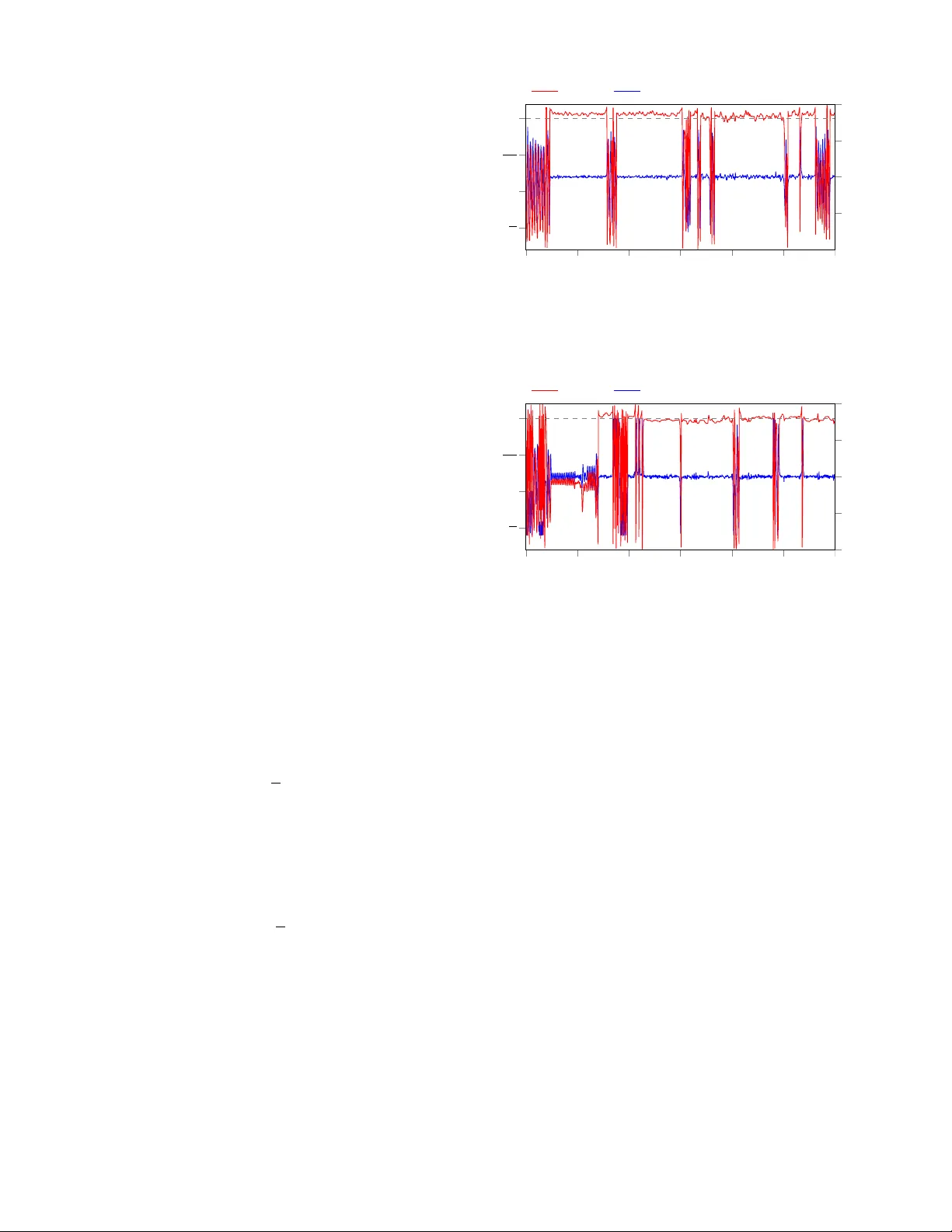
P artner Approximating Learners (P AL): Simulation-Accelerated Learning with Explicit P artner Modeling in Multi-Agent Domains ∗∗ Florian K ¨ opf ∗ , Alexander Nitsch ∗ , Michael Flad and S ¨ oren Hohmann Institute of Contr ol Systems (IRS) Karlsruhe Institute of T echnology (KIT) Karlsruhe, Germany florian.koepf@kit.edu, soeren.hohmann@kit.edu Abstract —Mixed cooperative-competiti ve control scenarios such as human-machine interaction with individual goals of the interacting partners are very challenging for reinfor cement learning agents. In order to contribute towards intuitive human- machine collaboration, we focus on problems in the continuous state and control domain wher e no explicit communication is considered and the agents do not know the others’ goals or con- trol laws but only sense their control inputs retrospecti vely . Our proposed framework combines a learned partner model based on online data with a reinf orcement learning agent that is trained in a simulated en vironment including the partner model. Thus, we over come drawbacks of independent learners and, in addition, benefit from a r educed amount of real world data r equired for reinf orcement learning which is vital in the human-machine context. W e finally analyze an example that demonstrates the merits of our pr oposed framework which learns fast due to the simulated envir onment and adapts to the continuously changing partner because of the partner appr oximation. Index T erms —Reinf orcement Learning, Mixed Cooperative- Competitive Contr ol, Machine Learning in Control, Opponent Modeling I . I N T R O D U C T I O N In numerous control problems such as robotics, intelligent manufacturing plants and highly-automated driving, sev eral so-called agents (e.g. machines and/or humans) are in volv ed and need to adapt to each other in order to improve their behavior . Allo wing the agents to pursue indi vidual, not nec- essarily opposing, goals by means of indi vidual re ward struc- tures leads to mixed cooperativ e-competitive [1] reinforcement learning (RL) problems. Although, especially in control prob- lems, the system dynamics is often known, the reward struc- tures and control laws of other agents are usually unknown to each agent. If the agents adapt their behavior during runtime, this leads to non-stationary en vironments from the point of view of each agent. Thus, rather than being ignorant concern- ing the presence of other agents, it is advisable to consider their influence explicitly [2]. Another challenge arising when control tasks are learned by means of RL is the lack of data ef- ficiency as much real-world data is required in order to obtain ∗ These authors contributed equally to this work. ∗∗ This work has been submitted to IEEE for possible publication. decent performance. Major successes in training an agent in simulated en vironments rather than solely based on real data hav e been reported by [3] and [4]. In simulated en vironments, powerful hardware can be used to speed up simulations and thus increase the rate of interactions without risk of erratic exploration. Howe ver , concerning the multi-agent case, RL based solely on simulations would not appropriately consider the other agents’ non-stationary behavior . In this work, we focus on control problems in continuous state and control spaces where no explicit communication or rew ard sharing is av ailable b ut the agents are solely able to sense or deduce the other agents’ control inputs after they ha ve been applied. In order to account for the above-mentioned challenges, we propose a general framew ork that combines the merits of maintaining a partner model that is constantly updated based on real data with learning in a simulated en- vironment. More precisely , each agent approximates a partner model that incorporates the aggregated controls of all other agents. This approximation is constantly updated based on real data in order to capture their changing behavior . Then, each agent simulates a virtual replica of the real control loop containing the system model, the partner approximation and his own control law . In this virtual simulation, the agent updates his control law by means of RL methods in order to improve the performance w .r .t. his reward function. The control la w learned in the virtual en vironment is then trans- ferred to the real control loop and the partner approximation is updated again in order to capture the other agents’ changes and reaction. That way , potentially non-stationary partners are steadily approximated and explicitly considered by the RL agent learning in a simulated en vironment. In the next section, we define our problem and the concept of partner approximating learners (P AL). Then, we place our framew ork in the context of related work before we propose our main topology . Finally , we give an example choice of the components and analyse our method by means of a swing-up task of an in verted pendulum. I I . P R O B L E M A N D PA RT N E R A P P R OX I M A T I N G L E A R N E R D E FI N I T I O N Consider a discrete-time system controlled by N agents that is gi ven in nonlinear state space representation x k +1 = f ( x k , u 1 ,k , . . . , u N ,k ) , where x k ∈ X ⊆ R n and u i,k ∈ U i ⊆ R q i are the continuous state and continuous control of agent i ∈ { 1 , . . . , N } . From the point of vie w of agent i , let u p i =  u | 1 . . . u | i − 1 u | i +1 . . . u | N  | be the aggregated control input of all other agents. Then, agent i aims to adapt his control la w π i : X → U i in order to maximize his long-term discounted rew ard R i = ∞ X k =0 γ k i r i ( x k , u i,k , u p i ,k ) = ∞ X k =0 γ k i r i ( x k , π i ( x k ) , π p i ( x k )) . (1) In this mixed cooperativ e-competitiv e setting with continuous state and control spaces, no explicit communication between the agents is allo wed. Each agent i maintains a model of the system dynamics f , either as a result of model design or approximated via e.g. recurrent neural networks. Furthermore, each agent senses the partners’ controls u p i ,k − 1 , i.e. after one step delay , as well as the system state x k and is aware of his own re ward function r i ( x k , u i,k , u p i ,k ) and discount factor γ i , but has no knowledge of the other agents’ rew ard functions r j ( · ) , j 6 = i and control laws π p i ( x k ) = u p i ,k . Based on this problem definition, the notion of partner approximating learners (P AL) is giv en as follows. Definition 1: A partner appr oximating learner (P AL ) is an RL agent in a multiagent setting acting in continuous state and control spaces that • does not explicitly communicate with other agents and does not know their reward structures and control la ws • is able to sense or deduce the other agents’ control inputs after they ha ve been applied • maintains and updates a model of the other agents’ aggregated control law (partner model) based on real data • updates his control law based on simulated data while explicitly incorporating the partner model. In the follo wing section, we outline related work before our proposed framew ork is introduced. I I I . R E L AT E D W O R K The idea to incorporate simulated data from a system model into the learning process of an RL agent was proposed in the Dyna architecture [5]. Extensions of this concept to use a simulated environment rather than solely learning from real data marked a breakthrough in order to cope with the sample complexity when using high-dimensional function approxi- mators in continuous control tasks. One example is the use of Normalized Advantage Functions (NAF) with Imagination Rollouts [6], which not only allows for the use of continuous state and control spaces, b ut accelerates learning by means of model-based simulated data that is additionally fed into the replay buf fer . Another example is gi ven by [4], where a com- plex dexterous hand manipulation task has successfully been learned in simulation based on Proximal Policy Optimization (PPO) [7] and transferred to a physical robot. On the multi-agent side, independent learners ha ve shown limited performance [2] due to the non-stationarity of the en vironment. In fully cooperative settings, optimistic learning such as hysteretic Q-learning [8] was proposed assuming that all agents tend to improve collectiv e rewards. Other approaches require explicit communication [9], [10] or share actor parameters [11], [12]. Partner modeling stri ves to av oid the disadv antages of independent learners without the neces- sity of communication or parameter sharing. In Self Other- Modeling [13], the agent updates his belief of the partners’ hidden goals and predicts the others’ controls inputs based on his o wn control law . In the work of [14], the maximum- likelihood is used to predict the partners’ future controls based on previous controls in finite state and control spaces under the requirement that the payoff matrix is known to all agents. Multi-agent Deep Deterministic Policy Gradient MADDPG [1] is a remarkable extension to DDPG [15], thus allowing continuous state and control spaces. MADDPG uses centralized training with decentralized execution. Thus, the Q- function of each agent not only depends on the state and his own control but also the controls of all other agents. In order to remove the assumption of knowing all agents’ control laws, it is suggested in [1, Section 4.2] to infer control laws of other agents. Usually , multi-agent RL algorithms do not explicitly assume knowledge of the system dynamics f and therefore learn only based on observ ed data. In contrast, our frame work benefits from kno wn system dynamics, which is often available in control engineering as a result of model design or can be approximated, and requires real data solely to update the partner model whereas the RL agent is able to explore and generate huge amounts of data in a virtual environment. Our framew ork proposed in the next section incorporates partner modeling into the paradigm to accelerate learning by using simulated data and can therefore be interpreted to extend powerful mechanisms such as the Dyna-architecture [5] or Imagination Rollouts [6] to the multi-agent case. I V . P RO P O S E D A D A P T I V E M I X E D C O O P E R A T I V E - C O M P E T I T I V E C O N T RO L L E R In this section, we introduce the topology of the proposed Partner Approximating Learner frame work (P AL-frame work), which can be used with v arious partner identification and RL algorithms due to its modularity . W e refer to all controllers implemented in the P AL-framew ork as Partner Approximating Learners (P ALs). Our frame work consists of three main com- ponents that can be seen in Fig. 1: the identification which approximates all partners’ aggregated control law π p i with a model ˆ π p i and the internal simulation where RL is used to improv e the last component namely the contr ol law π i which is applied to the real physical system to be controlled. In the following, the components will be explained in more detail. internal simulation reality identification rew ard RL agent controller π i partners π p i sim. system real system ˆ u p i ˆ x ˆ u i u i u p i x x u p i partner model ˆ π p i Fig. 1: Structure of the proposed framew ork. Each agent iden- tifies an aggregated partner model from online data, optimizes his control la w based on the partner model and system model by means of RL in the internal simulation and transfers the learned control law to the controller in reality . A. Online partner identification with experience r eplay T o be able to improve the own control law π i tow ard a higher long-term reward R i , the behavior of the partners must be taken into account. W e therefore continuously identify and improv e a model ˆ π p i : X → U ˆ p i of π p i in order to predict the aggregate control input u p i ,k of all partners from the current state x k . Note howe ver , that π p i is not always fixed and might change, e.g. because the partners are learning as well. Thus, the model ˆ π p i should be a flexible and powerful function approximator in order to accurately capture a wide range of possible partner control laws. Supervised learning algorithms typically require a lot of training data before any useful approximation of the target is obtained. Due to the f act that the data has to be obtained from interactions of the partners with the system, the rate of new information about the partners’ behavior is quite lo w . Additionally , using only the newest set of input-output data ( x k , u p i ,k ) for training leads to a high v ariance in the direction of the applied updates to the models which often leads to unstable learning algorithms [16]. Both the relative scarcity of data and the high variance of updates also pre vented the use of deep neural networks in RL for many years. A breakthrough to both problems was introduced to deep RL by [16] in the form of e xperience replay (ER). Instead of training on only the latest experience, m RL samples are chosen from the replay buf fer B RL uniformly at random (u.a.r .) and form the mini- batch, which is used for training. Because both online identification and deep RL exhibit these problems, we adapt experience replay for the use in online identification. T o this end, we save the input-output data of the partner as experiences e k = ( x k , u p i ,k ) into an identification b uffer B ID . T o update the approximate model of the partner , we pick m ID experiences from the buf fer and use a supervised learning algorithm that is appropriate for the specific task. The size of the buf fer should be large enough to have a high chance of holding information about dif ferent regions of the state space and thus capturing nonlinearities in partner model supervised learning experience replay identification buf fer x u p i identification Fig. 2: Online identification. Each time step k , the state x k and control input of the partners u p i ,k are stored in the iden- tification buf fer B ID . A mini-batch is formed by picking m ID experiences using an applicable experience replay algorithm and the model ˆ π p i of the partners’ behavior π p i is improved. the identification step. Limiting it in size is ho wev er not only a memory requirement, but helps to discard experiences that are outdated and thus do not capture the current behavior of the potentially changing partner . Even improved ER algorithms which differ in the way the experiences are drawn from B ID , such as prioritized experience replay (PER) [17] and combined experience replay (CER) [18], can be used directly as long as they do not take the reward of an experience into account (there is no rew ard associated with the input-output data e k = ( x k , u p i ,k ) of the partner). T o use PER, the priorities are weighted according to the prediction error rather than the TD error . Fig. 2 shows the different components of the identification part of the controller . B. Internal simulation The core idea of the P AL-framework lies within the internal simulation that the controller runs in order to improve its control law . It consists of two parts, a virtual replica of the real control loop and an RL agent acting on this replica. 1) V irtual replica: In order to capture the interactions of the real control loop, the three components of “reality” in Fig. 1 have to be known. The controller’ s behavior π i and the system dynamics are both known, while the partners’ behavior π p i is not. This is where the approximate partner model ˆ π p i (see Section IV -A) is used. W e are no w able to simulate the behavior of the real control loop offline and typically much faster , with no wear of the hardware and without cumbersome and costly RL on the physical system. 2) Reinfor cement learning algorithm: W ith a simulation of the real control loop at hand, RL can be applied in a straightforward way , when the system and approximate partner model are combined into a single Mark ov De- cision Process (MDP) with state space X , action space U i , system dynamics f  ˆ x ˆ k , ˆ u i, ˆ k , ˆ π p i ( ˆ x ˆ k )  , rew ard function r i  ˆ x ˆ k , ˆ u i, ˆ k , ˆ π p i ( ˆ x ˆ k )  and discount factor γ i , where ˆ k denotes the time step in the simulation. In this auxiliary MDP , the RL agent chooses simulated controls ˆ u i, ˆ k and obtains the resulting simulated state ˆ x ˆ k of the simulated system. In addition, the agent experiences a reward r i  ˆ x ˆ k , π i ( ˆ x ˆ k ) , ˆ π p i ( ˆ x ˆ k )  . Based on these experiences, which are usually stored in a replay buf fer B RL , the agent improves his control la w . The complete setup of the simulated control loop can be seen in Fig. 3 for the example of an actor-critic RL agent, where the critic estimates replay buf fer internal simulation RL agent training critic actor rew ard r ˆ u i ˆ x ˆ x ˆ x ˆ u p i partner model sim. system Fig. 3: An RL agent improv es his control law in the internal simulation based on the partner model and system dynamics. the long-term re ward and the actor represents the control la w . Note that for some RL algorithms, the partner model ˆ π p i may additionally be used directly by the RL agent, e.g. in the case of MADDPG [1]. C. Contr ol law π i The control law learned in simulation can then be used as the control law of the controller acting on the physical system (i.e. “reality” in Fig. 1). The representation of the control la w π i that acts on the physical system therefore depends on the kind of RL agent that is used in the internal simulation. Since the formulation of the problem is done in discrete time, π i will be used every timestep k to calculate u i,k for the duration of the next timestep. V . E X P E R I M E N T S In this section, we giv e the example system that is used in order to demonstrate the effecti veness of the proposed topology , define concrete algorithms for the experiments and discuss results. A. Example system Because of the relev ance both in control theory [19] and machine learning [20] literature, a pendulum swing-up task is selected. T o easily and reproducibly test the potential of the proposed controller, the “real, i.e. physical, system is replaced by a separate simulation, not to be confused with the internal simulation implemented by P ALs. The pendulum has a two- dimensional state space, an angle ϕ , where ϕ = 0 = 2 π is defined to be the upright position, and an angular velocity ω and two agents are able to control the pendulum simul- taneously . Both control variables u 1 and u 2 that represent a momentum applied to the pendulum are clipped to the range of [ − 5 , +5] rad / s 2 which necessitates a swing-up of the pendulum. The pendulum model is based on the pendulum from OpenAI Gym [21] and modified to additionally allow a second agent to apply torque to the pendulum. At first, the goal is for both controllers to swing-up and hold the pendulum vertically , later we shift the goal to an inclined position. On reset, the pendulum starts at a random state within ϕ ∈ ( − π , + π ] rad , ω ∈ ( − 8 , +8] rad / s , which means it has some potential and/or kinetic energy at initialization. The nonlinear system equations are giv en by x k +1 =  ϕ ω  k +1 =  ϕ + ω · ∆ t ω + ( − 3 g 2 l · sin( ϕ + π ) + 3 ml 2 ) · ∆ t  k +  0 0 ∆ t ∆ t  ·  u 1 u 2  k , where ∆ t = 0 . 05 s , g = 10 m / s 2 , m = 1 kg and l = 1 m . In the follo wing, concrete algorithms will be chosen to implement P ALs. B. DDPG-P AL T o approximate the partners, we use a multilayer perceptron (MLP) to be able to capture highly nonlinear control laws π p i . In order to train this partner model ˆ π p i , we use CER [22], as it uses new information right when it is available and is fairly robust to the size of the replay buffer . For the RL agents, the Deep Deterministic Policy Gradient (DDPG) algorithm [15] is chosen. This makes the use of continuous state and control spaces possible. Because of the actor-critic nature of the DDPG algorithm, the control law can also be easily used on the real system, since it is directly av ailable in the form of the actor . W e will refer to this specific P AL implementation as DDPG-P AL. The choice of optimizers, learning rates and other hyperparameters are giv en in the supplementary details in Appendix A. C. Examined contr oller setups In order to examine the functionality of DDPG-P ALs, the internal simulation, the partner approximation and the RL agent hav e to work properly . T o examine whether all of these components contribute to the proper functioning, several experiments are conducted and presented in the follo wing. Since we are focusing on interacting agents, both controllers are learning. The metrics that are reported are averaged ov er ten test runs and the plots are from one of the two runs that were closest to the median. The four dif ferent setups that are examined are defined as follo ws. 1) Baseline (no internal simulation; no explicit identifica- tion): The direct b ut naiv e way of using RL for a cooperative swing-up task follo ws the independent learner paradigm (cf. [2]). In this case, both the controller and its partner are regular DDPG agents interacting with the same physical environment without using an internal simulation. In order not to withhold information that the DDPG-P AL possesses, the baseline agents can measure the delayed output of each other and treat it like a third state of the system. For the agent, this can reduce the perceiv ed instationarity of the MDP containing an adapti ve partner [1]. 2) Oblivious DDPG-agents in a simulated en vironment (using an internal simulation; identification disabled): Since both agents, while initialized differently , hav e the same goal, it might be possible for them to achieve the swing-up without knowledge of the other controller . T o test if the identification is indeed improving the agents’ performance, we use the internal simulation while disabling the identification. This results in each controller learning in an internal simulation which only incorporates the system model. They learn as if there were no partner influencing the system, with no way of realizing that there is, which is why we call them oblivious DDPG-agents. 3) DDPG-P ALs (using an internal simulation and identifi- cation): In order to improve both learning time and quality through simulated experience and a partner model, we use DDPG-P AL for both partners. Therefore, this controller setup represents an example of our proposed P AL-architecture. For the scenarios above, the goal of swinging up the pendulum and holding it upright is expressed with the rew ard function r ( x k , u k ) = − ϕ 2 k − 0 . 1 ω 2 k − 0 . 01 u 2 k for both agents, i.e. u k ∈ { u 1 ,k , u 2 ,k } . It punishes the control effort u 2 k , the deviation from the vertical position ϕ = 0 = 2 π and the angular velocity ω . 4) DDPG-P ALs with differ ent r ewar d functions: While the aforementioned settings serve to examine the adv antages of the P AL-architecture, the fourth experiment uses partners with dif ferent re ward functions. This is moti vated by the case of human-robot-collaboration, where, although goals are typically aligned, different humans might prefer different ways of achieving the goal. As an example, imagine the task for a human to transport a piece of equipment from A to B with support by a robot. Understandably , taller people might hav e different preferences regarding the height it should be transported at compared to shorter people. A suitable robot controller would ideally both realize and account for those preferences and thus learn to support different human partners differently when transporting the piece of equipment as long as this aligns with its own goals. T o mimic this situation, we use two DDPG-P ALs with slightly different reward functions. Here, the machine con- troller (agent 1), trying to cooperate with the partner (agent 2), uses the rew ard r 1 ( x k , u 1 ,k ) = −  | ϕ k | − π 4  2 − 0 . 1 ω 2 k − 0 . 1 u 2 1 ,k . (2) Thus, agent 1 has two optima for the pendulum position, ϕ opt and − ϕ opt . Note that ϕ opt ≈ 0 . 3 is the angle at which the negati ve reward caused by the de viation from π / 4 and the constant control effort to hold this position are balanced. On the other hand, the partner (e.g. representing the human) uses r 2 ( x k , u 2 ,k ) = −  ϕ k − π 4  2 − 0 . 1 ω 2 k − 0 . 1 u 2 2 ,k . (3) This means he would like to swing-up the pendulum and hold it at ϕ opt . The second optimum for agent 1 at − ϕ opt thus leads to a lo wer rew ard for agent 2. T o ease the swing-up for this task, the limits of u 1 and u 2 are widened to [ − 10 , 10] rad / s 2 . D. Results As is depicted in Fig. 4, baseline DDPG-agents swing-up the pendulum towards the vertical position ϕ = 0 = 2 π at around 1220 s for the first time. In addition to taking relativ ely − 10 − 5 0 5 10 ω in rad/s 1200 1250 1300 1350 1400 1450 1500 π 2 π 3 π 2 2 π t in s ϕ in rad angle ϕ angular velocity ω Fig. 4: Cooperativ e swing-up with two baseline agents. Note the shifted time axis. − 10 − 5 0 5 10 ω in rad/s angle ϕ 0 50 100 150 200 250 300 π 2 π 3 π 2 2 π t in s ϕ in rad angle ϕ angular velocity ω Fig. 5: T wo oblivious DDPG-agents performing the swing-up task without knowledge of each other . long until the first successful swing-up is performed, holding the pendulum upright is very unstable and it can be seen that the pendulum tips over multiple times with no significant improv ement. Considering the oblivious DDPG-a gents , Fig. 5 sho ws that ev en without the identification a swing-up can generally be learned much faster in the simulated en vironment compared to the baseline. Ho wev er , because the impact of the partner is ignored, the pendulum can not be held upright for longer periods of time. This leads to an average reward per second of − 61 . 8 over all runs in the first 300 s whereas for the baseline the av erage rew ard in this time is − 1104 and clearly much worse as the pendulum is not held in the upright position at all during this time. Fig. 6 re veals that the swing-up is successful after just 70 s when using DDPG-P ALs . In addition, it can be seen that the pendulum is held upright more stable compared to the baseline and the oblivious DDPG-agents and is easily re-erected after tipping over . The cooperating DDPG-P ALs achiev e an average rew ard per second of − 36 , 79 which is a significant improve- ment compared to the obli vious DDGP-agents which do not include the partner model. These results show that not only the internal simulation, but also the identification significantly 0 50 100 150 200 250 300 − 10 − 5 0 5 10 ω in rad/s 0 50 100 150 200 250 300 π 2 π 3 π 2 2 π t in s ϕ in rad angle ϕ angular velocity ω Fig. 6: Both agents learn using DDPG-P AL including internal simulations. 0 50 100 150 200 250 300 − 10 − 5 0 5 10 ω in rad/s angle ϕ 0 50 100 150 200 250 300 π 2 π 3 π 2 − ϕ opt ϕ opt t in s ϕ in rad angle ϕ angular velocity ω Fig. 7: T wo DDPG-P ALs with different goals agree on the optimum that suits both. improv es the results. For DDPG-P ALs with differ ent re ward functions , Fig. 7 shows that swinging up the pendulum is also achieved quite fast. At t = 75 s , the pendulum is held vertically , which already leads to fairly high reward. This vertical position is, howe ver , not the optimum for either of the controllers. Right after tipping over at roughly t = 130 s , they agree on the optimal position at around ϕ opt . E. Discussion The results above indicate that the desired behavior can successfully be learned by P ALs. In order to make broader claims about the applicability especially in the case of P ALs with dif ferent re ward functions, it is necessary to show that agent 1 has indeed learned to prefer ϕ opt ov er − ϕ opt , ev en though this does not follo w directly from r 1 . Instead, prefer- ring ϕ opt is better for agent 1 because agent 2 is uncooperati ve at − ϕ opt , which leads to a lower reward for agent 1 in the region around − ϕ opt . The preferences of agent 1 can not only be found by experimentation, but explicitly in the DDPG critic, i.e. the action-value function Q 1 ( x , u 1 ) , that is used in the internal simulation. Removing the dependency on the control (i.e. action), we get the state-value function V 1 ( x ) = max u 1 ( Q 1 ( x , u 1 )) , which allows us to compare the value that the agent assigns to the two states at ± ϕ opt (with ˙ ϕ opt = 0 ). As reference, we perform ten runs where agent 1 has his partner approximation disabled, i.e. follows the oblivious-agent mechanism. This leads to the average v alues of V 1 ( x = ( − ϕ opt , 0)) = − 35 . 52 and V 1 ( x = (+ ϕ opt , 0)) = − 34 . 69 which makes a difference of only 0 . 83 , meaning that the controller does not significantly prefer one of the states over the other . Furthermore, note that this v alue is solely based on the estimation of the agent in the internal simulation and not on actual rewards. W ith partner approximation disabled, the MDP in the internal simulation is less complex because the influence of the partner is missing. This leads to the agent estimating higher re wards than he would actually get when acting in the real world where the partner influences the system as well (cf. the oblivious DDPG-agents that suffer from the lack of an appropriate partner model). When using the full DDPG-P AL algorithm with part- ner approximation, the distinction becomes much more significant as V 1 , P AL ( x = ( − ϕ opt , 0)) = − 47 . 55 and V 1 , P AL ( x = (+ ϕ opt , 0)) = − 39 . 83 and reflects reality much better where − ϕ opt is penalized. Thus, the agent dev eloped understanding of the situation. This indicates that P ALs can indeed learn the preferences of their partner and subsequently improv e the control law to wards goal-oriented cooperation. V I . C O N C L U S I O N This work introduces a framework named P artner Approx- imating Learners (P AL-framew ork) which combines learning the partners’ behavior in mixed cooperative-competiti ve set- tings under restricted information with deep RL in a simulated en vironment. The frame work offers tw o major benefits over independent learners merely training on online data. On one hand, maintaining and constantly updating an e xplicit model of the partners’ aggregated control law takes their influence into consideration and allows the agents to adapt to each other . On the other hand, P ALs learn in a simulated en vironment where the current partner model is explicitly used. Thus, P ALs reduce wear on the system explore the state space more safely , while relying on the latest partner model. After proposing our framew ork, we show its merits by an example of a pendulum swing-up task. Here, utilizing the simulated en vironment rather than simply working on online data significantly speeds up learning. Furthermore, maintaining a partner model improves the performance. Finally , two DDPG-P ALs, where one is indif- ferent to tw o states and the other prefers one state o ver another , successfully assess the situation and agree on a reasonable solution despite the challenging setting of the agents having different reward functions. R E F E R E N C E S [1] R. Lo we, Y . W u, A. T amar , J. Harb, O. P . Abbeel, and I. Mor- datch, “Multi-agent actor-critic for mixed cooperative-competiti ve en- vironments, ” in Advances in Neural Information Pr ocessing Systems , pp. 6379–6390, 2017. [2] L. Matignon, G. J. Laurent, and N. Le Fort-Piat, “Independent rein- forcement learners in cooperative marko v games: A survey regarding coordination problems, ” The Knowledge Engineering Review , v ol. 27, no. 1, pp. 1–31, 2012. [3] A. Broka w , “Google hooked 14 robot arms together so the y can help each other learn, ” 2016. [4] M. Andrycho wicz, B. Baker, M. Chociej, R. Jozefo wicz, B. McGrew , J. Pachocki, A. Petron, M. Plappert, G. Powell, A. Ray , J. Schneider, S. Sidor, J. T obin, P . W elinder , L. W eng, and W . Zaremba, “Learning dexterous in-hand manipulation, ” Arxiv .or g , vol. 1808.00177, 2018. [5] R. S. Sutton, “Dyna, an integrated architecture for learning, planning, and reacting, ” ACM SIGART Bulletin , vol. 2, no. 4, pp. 160–163, 1991. [6] S. Gu, T . Lillicrap, I. Sutskever , and S. Levine, “Continuous deep q- learning with model-based acceleration, ” in International Confer ence on Machine Learning , pp. 2829–2838, 2016. [7] J. Schulman, F . W olski, P . Dhariwal, A. Radford, and O. Klimov , “Proximal policy optimization algorithms, ” CoRR , vol. abs/1707.06347, 2017. [8] L. Matignon, G. J. Laurent, and N. Le Fort-Piat, “Hysteretic q-learning: An algorithm for decentralized reinforcement learning in cooperative multi-agent teams, ” in 2007 IEEE/RSJ International Conference on Intelligent Robots and Systems , pp. 64–69, 2007. [9] J. Foerster, I. A. Assael, N. d. Freitas, and S. Whiteson, “Learning to communicate with deep multi-agent reinforcement learning, ” 30th Confer ence on Neural Information Pr ocessing Systems , 2016. [10] S. Sukhbaatar , A. Szlam, and R. Fergus, “Learning multiagent com- munication with backpropagation, ” in Advances in Neural Information Pr ocessing Systems 29 , pp. 2244–2252, Curran Associates, Inc, 2016. [11] J. K. Gupta, M. Egorov , and M. Kochenderfer , “Cooperative multi-agent control using deep reinforcement learning, ” in Autonomous Agents and Multiagent Systems (G. Sukthankar and J. A. Rodriguez-Aguilar, eds.), vol. 10642 of Lecture Notes in Computer Science , pp. 66–83, Cham: Springer International Publishing, 2017. [12] M. J. Hausknecht, Cooperation and Communication in Multiagent Deep Reinfor cement Learning . Phd thesis, University of Austin, T exas, USA, 2016. [13] R. Raileanu, E. Denton, A. Szlam, and R. Fergus, “Modeling oth- ers using oneself in multi-agent reinforcement learning, ” Arxiv .org , vol. 1802.09640v3, 2018. [14] J. Foerster , R. Y . Chen, M. Al-Shediv at, S. Whiteson, P . Abbeel, and I. Mordatch, “Learning with opponent-learning awareness, ” in Pr oceed- ings of the 17th International Confer ence on A utonomous Agents and MultiAgent Systems , AAMAS ’18, pp. 122–130, 2018. [15] T . P . Lillicrap, J. J. Hunt, A. Pritzel, N. Heess, T . Erez, Y . T assa, D. Silver , and D. Wierstra, “Continuous control with deep reinforcement learning, ” Arxiv .org , vol. 1509.02971v5, 2015. [16] V . Mnih, K. Kavukcuoglu, D. Silver, A. Graves, I. Antonoglou, D. Wier - stra, and M. Riedmiller , “Playing atari with deep reinforcement learn- ing, ” 2013. [17] T . Schaul, D. Horgan, K. Gregor, and D. Silver , “Universal value func- tion approximators, ” in International Conference on Machine Learning , pp. 1312–1320, 2015. [18] K. Zhang, H. Zhang, G. Xiao, and H. Su, “Tracking control optimization scheme of continuous-time nonlinear system via online single network adaptiv e critic design method, ” Neurocomputing , vol. 251, pp. 127–135, 2017. [19] K. J. ˚ Astr ¨ om and K. Furuta, “Swinging up a pendulum by ener gy control, ” Automatica , vol. 36, no. 2, pp. 287–295, 2000. [20] S. Adam, L. Busoniu, and R. Babuska, “Experience replay for real-time reinforcement learning control, ” IEEE T ransactions on Systems, Man, and Cybernetics, P art C (Applications and Reviews) , vol. 42, no. 2, pp. 201–212, 2012. [21] G. Brockman, V . Cheung, L. Pettersson, J. Schneider, J. Schulman, J. T ang, and W . Zaremba, “Openai gym, ” Arxiv .org , v ol. 1606.01540, 2016. [22] S. Zhang and R. S. Sutton, “ A deeper look at experience replay , ” Arxiv .or g , vol. 1712.01275, 2017. A P P E N D I X The hyperparameters of the identification algorithm as well as the RL agent are giv en below . T ABLE I: Hyperparameters of the identification. hyperparameter value time steps between ident. updates 1 learning episodes per ident. update 4 number of hidden layers 3 neurons per hidden layer 16 size of identification buf fer B ID last 100 s of “reality” experience replay CER [18] training data per ident. update 10% of buf fer mini batch size 20 initial weights hidden layer u.a.r . ∈ [ − 1 , 1] initial weights output layer u.a.r . ∈  − 10 − 4 , 10 − 4  activ ation function hidden layer sigmoid activ ation function output layer linear optimizer Adam, learning rate 0 . 01 , β 1 = 0 . 9 , β 2 = 0 . 999 , no gradient clipping, decay , fuzz factor or AMSGrad error metric MSE size of validation set 0 shuffle mini batch before training true T ABLE II: Hyperparameters of the DDPG agents. Here, A/C stands for “actor and critic” hyperparameter value time steps between RL updates 2 size of replay buf fer B RL last 10 s of “reality” length episode RL training 10 s simulated time, m RL = 200 number of hidden layers A/C 3 neurons per hidden layer actor 16 neurons per hidden layer critic 32 activ ation f. hidden layer A/C sigmoid activ ation f. output layer A/C linear initial weights all layers A/C u.a.r . ∈ [ − 1 , 1] optimizer A/C Adam, learning rate 0 . 001 , β 1 = 0 . 9 , β 2 = 0 . 999 gradient clipping = 1 . 0 no decay , fuzz factor or AMSGrad experience replay u.a.r . [15] discount factor γ 0 . 99 batch size 32 warm up A/C 100 error metric MAE target network update rate 0 . 001 exploration Ornstein-Uhlenbeck with θ = 0 . 15 , µ = 0 , σ = 0 . 3