Computationally Efficient Distributed Multi-sensor Fusion with Multi-Bernoulli Filter

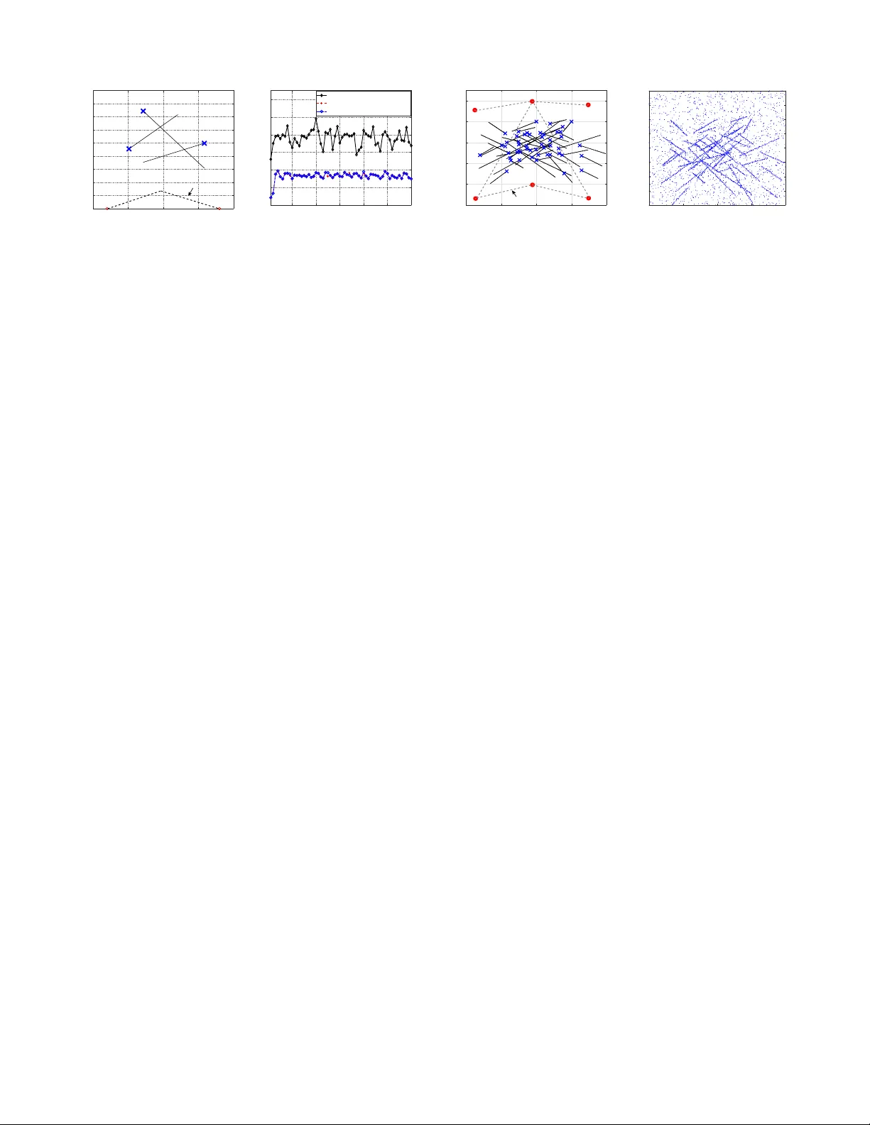
Computationally Ef ﬁcient Distrib uted Multi-sensor Fusion with Multi-Bernoulli Filter W ei Y i, Suqi Li ∗ , Bailu W ang, Reza Hoseinnezhad and Lingjiang K ong Abstract —This paper proposes a computationally efﬁcient al- gorithm f or distrib uted fusion in a sensor netw ork in which multi- Bernoulli (MB) ﬁlters are locally running in e very sensor node for multi-target tracking. The generalized Covariance Intersection (GCI) fusion rule is employed to fuse multiple MB random ﬁnite set densities. The fused density comprises a set of fusion hypotheses that gro w exponentially with the number of Bernoulli components. Thus, GCI fusion with MB ﬁlters can become computationally intractable in practical applications that in volve tracking of even a moderate number of objects. In order to accel- erate the multi-sensor fusion procedure, we derive a theoretically sound approximation to the fused density . The number of fusion hypotheses in the resulting density is signiﬁcantly smaller than the original fused density . It also has a parallelizable structure that allows multiple clusters of Bernoulli components to be fused independently . By carefully clustering Bernoulli components into isolated clusters using the GCI divergence as the distance metric, we pr opose an alter native to build exactly the approximated density without exhaustively computing all the fusion hypotheses. The combination of the proposed approximation technique and the fast clustering algorithm can enable a novel and fast GCI- MB fusion implementation. Our analysis shows that the pro- posed fusion method can dramatically r educe the computational and memory requir ements with small bounded L 1 -error . The Gaussian mixture implementation of the proposed method is also presented. In various numerical experiments, including a challenging scenario with up to forty objects, the efﬁcacy of the proposed fusion method is demonstrated. I . I N T RO D U C T I O N D ISTRIBUTED Multi-sensor Multi-object Tracking (DMMT) technology is recently advocated in the information fusion community , since it generally beneﬁts from lo wer communication costs and immunity to single-node fault, compared with optimal centralized fusion solutions. In practice, the correlations between the posterior densities from different sensors are usually unknown, and this makes it very challenging to devise DMMT solutions. The optimal solution to this problem has been proposed by Chong et al. [1], b ut the heavy computational burden of extracting the common information can rule out this solution in many applications. A suboptimal solution with demonstrated tractability has been formulated based on the Generalized Cov ariance Intersection (GCI) method proposed by Mahler [2]. Essentially , GCI is the generalization of Cov ariance Intersection (CI) [3]. Compared to the CI fusion rule, which mainly utilizes the ﬁrst and second W . Y i, S. Li, B. W ang and L. Kong are with the School of In- formation and Communication Engineering, the University of Electronic Science and T echnology of China. (Suqi Li is the corresponding author , Email:qi qi zhu1210@163.com) R. Hoseinnezhad is with the School of Engineering, RMIT Uni versity , V ictoria 3083, Australia. order statistical characteristics of the single-object densities, the GCI fusion rule is capable to fuse multiple full multi- object densities with unkno wn correlations among sensor nodes, while intrinsically av oiding the double counting of common information [4]. The GCI fused multi-object density is also named as Exponential Mixture Density (EMD) [5], [6] or Kullback-Leibler A verage (KLA) [7]. Clark et al. [8] deri ved tractable implementations of the GCI fusion rule for especial cases where the multi-object distributions are Poisson, independent identically distributed (i.i.d.) clusters and Bernoulli distributions. Utilizing these formulations, the GCI fusion method can be implemented for distributed fusion in sensor networks where the Probability Hypothesis Density (PHD)/Cardinalized PHD (CPHD) ﬁlter or the Bernoulli ﬁlter are running locally in ev ery sensor node. Battistelli et al. [7] and Guldogan [9] proposed the Gaus- sian Mixture (GM) implementation of distributed fusion with CPHD ﬁlter and Bernoulli ﬁlter , respectively . Furthermore, a consensus approach to distributed multi-object tracking was ﬁrst introduced in [7], with which the GCI fusion can be implemented in a fully distributed manner . The Sequential Monte Carlo (SMC) implementation of the GCI fusion with CPHD ﬁlter was proposed by Uney et al. [5]. Compared with PHD [10], [11] and CPHD [12]–[15] ﬁlters, the Multi-Bernoulli (MB) ﬁlter [15], [16] can be more efﬁ- cient and accurate in problems that require object indi vidual existence probabilities. The performance of the MB ﬁlters has been well demonstrated in a wide range of practical monitoring problems such as radar tracking [17], video and audio tracking [16], [18], sensor control [19], [20], and acoustic sensor tracking [21]. In addition, a number of novel extensions of the MB recursion have also been in vestigated. Examples include the multiple model multi-Bernoulli ﬁlter proposed to cope with maneuvering objects [22], a robust multi-Bernoulli ﬁlter that can accommodate an unknown non-homogeneous clutter and detection proﬁle [23], a joint multi-object estimator for multi- Bernoulli models [24], and a few enhanced multi-Bernoulli ﬁlters [25], [26]. The generalization of MB ﬁlters to the DMMT problem was ﬁrstly in vestigated in [27], where a distributed fusion algorithm based on GCI fusion rule (called GCI-MB in this paper) is proposed. While the enhanced performance of the GCI- MB fusion has been demonstrated [27], its major drawback is the hea vy computational cost that increases e xponentially with the number of objects in the surveillance area. For the DMMT ov er a sensor network, it is of paramount importance to reduce the local (in-node) computational e xpenses as much as possible, since in the typical distributed sensor networks, 2 each node usually has limited processing po wer and energy resources. In this paper, the computations in volved in GCI-MB fusion are inv estigated, showing that the major contributor to the heavy computational burden is the exhausti ve calculation of the weights and fused single-object densities of the GCI- MB fusion hypotheses, noting that the number of hypotheses increases super-exponentially with the number of objects. This observation provides the insight that leads to a novel compu- tationally efﬁcient and naturally parallelizable implementation of the GCI-MB fusion. The major contributions are summarized as follows: 1) Devising a principled appr oximation to the fused den- sity : By discarding all the insigniﬁcant GCI-MB fusion hypotheses with negligible weights, then normalizing the rest of hypotheses, we obtain a principled approximation to the original fused density . This approximation not only consists of signiﬁcantly smaller number of fusion hypotheses but also enjoys an appealing structure: it can be factorized into several mutually independent and smaller size multi-object densities that lead to a principled independence approximation. Each of these factorized densities are sho wn to be equally returned by the GCI- MB fusion performed with a partial cluster of entire Bernoulli components. W e also quantify the approxima- tion error by deri ving the L 1 -error [28] between the original density and the approximated one, and show that it is reasonably small, and indeed, negligible for many practical applications. 2) F ast clustering of the Bernoulli components : The main challenge in obtaining the approximation is to truncate all the insigniﬁcant GCI-MB fusion hypotheses without computing them all in an e xhaustiv e manner . T o this end, by carefully clustering the Bernoulli components into isolated clusters according to a distance metric, i.e., GCI di vergence, and then discarding the hypotheses of the association pairs of Bernoulli components from different isolated clusters among sensors, one can build exactly the independence approximation without exhausti vely com- puting all the terms. By modeling the underline data structure of Bernoulli components among all sensors as a undirected graph, the clustering problem is tantamount to seeking connected components of a undirected graph dynamically , and can be solved by the disjoint-set data structure based fast solver with a computational cost that is only polynomial in the number of Bernoulli components. 3) Computationally efﬁcient GCI-MB fusion : The combina- tion of the independence approximation and the fast clus- tering algorithm can enable a computationally ef ﬁcient fu- sion algorithm. The fast clustering algorithm is employed at an early stage to obtain the approximated density . Then by utilizing the structure of the approximated density , GCI fusion is performed within each smaller clusters of Bernoulli components independently and in a parallelized manner , namely , via performing fusion between each pair of the factorized multi-object densities among sensors. The GM implementation of the proposed fast GCI-MB fusion is also presented. In numerical results, the ef ﬁciency and accurac y of the pro- posed fast GCI-MB fusion algorithm with GM implementation is tested in a challenging scenario with up to forty objects. Preliminary results hav e been published in the conference paper [29]. This paper presents a more complete theoretical and numerical study . The rest of the paper is organized as follows. Background material and notation are introduced in Section II. The GCI- MB fusion is brieﬂy revie wed and its computational in- tractability is discussed in Section III. Section IV de votes to the dev elopment of the proposed distributed fusion algorithm with MB ﬁlter based on the independence approximation and the fast clustering algorithm. Section V presents the GM implementation of the proposed GCI-MB fusion algorithm, including the algorithm pseudocode, and the analysis of its computational complexity . Section VI demonstrates the effec- tiv eness of the proposed fusion algorithm via various numer- ical experiments. Concluding remarks are ﬁnally provided in Section VII. I I . B AC K G R O U N D A N D N OTA T I O N Consider a sensor network which is constructed by a set of sensor nodes, s = 1 , · · · , N s . Each sensor node is link ed with its neighbours to exchange information, and is assumed to be equipped with some limited processing, memory and other electronic hardw are for sensing, signal processing and communication. T o describe the statistics of unkno wn and time-varying number of objects, the multi-object state at time k is nat- urally represented as a Random F inite Set (RFS) [11], [30] X k = { x k 1 , x k 2 , . . . , x k n } ∈ F ( X ) , where X is the space of single-object states, and F ( X ) is the collection of all ﬁnite subsets of X . Also, F n ( X ) denotes the collection of all ﬁnite subsets of X with the cardinality n . At each time step k , each sensor node s receiv es the observations of multiple objects, denoted by Z k s = { z k 1 ,s , · · · , z k m,s } ∈ F ( Z ) , where Z is the space of observations, and F ( Z ) is the collection of all ﬁnite subsets of Z . Let Z 1: k s = ( Z 1 s , . . . , Z k s ) denotes the history of observations from time 1 to time k at sensor s . A. Distributed multi-object trac king DMMT for a sensor network usually consists of three stages described as follow: – Local ﬁltering : Each node s collects observations of multiple objects Z k s at each time step k , and performs local ﬁltering based on the multi-object Bayesian recursion [11]. – Information e xchange: Each sensor node exchanges the multi-object posteriors with its neighbours via communication links. – Fusion of posteriors: Each node performs a fusion oper- ation to combine its locally computed posterior with the ones communicated by its neighbours. 3 B. Local ﬁltering using multi-Bernoulli ﬁlters 1) Multi-Bernoulli distribution: An RFS X distributed ac- cording to an MB distribution is deﬁned as the union of M independent Bernoulli RFSs X ( ` ) [2], X = M [ ` =1 X ( ` ) . (1) The MB distribution is completely characterized by a set of parameters { ( r ( ` ) , p ( ` ) ) } M ` =1 , where r ( ` ) denotes the existence probability and p ( ` ) ( · ) denotes the probability density of the ` -th Bernoulli RFS, or Bernoulli component. The multi-object probability density of an MB RFS is given by [2], π ( { x 1 , . . . , x n } ) = X 1 ≤ i 1 6 = ... 6 = i n ≤ M Q ( i 1 , ··· ,i n ) n Y j =1 p ( i j ) ( x j ) (2) where n = { 1 , · · · , M } and Q ( i 1 , ··· ,i n ) = M Y ` =1 (1 − r ( ` ) ) n Y j =1 r ( i j ) 1 − r ( i j ) . (3) In addition to (2), another equi valent form of MB distrib ution could be expressed as [27] π ( { x 1 ,. . .,x n } ) = X σ X I ∈F n ( L ) Q I n Y i =1 p ([ I ] v ( i )) ( x σ ( i ) ) (4) where L , { 1 , . . . , M } is a set of index es numbering Bernoulli components, I is the set of indexes of densities, σ denotes one possible permutation of I , σ ( i ) denotes the i -th element of the permutation, the summation P σ is taken over all permutations on the numbers { 1 , · · · , n } , [ I ] v is a vector constructed by sorting the elements of the set I , and Q I = Y ` 0 ∈ I r ( ` 0 ) Y ` ∈ L \ I (1 − r ( ` ) ) . (5) Hereafter , each Bernoulli component ` ∈ L , paramerized by ( r ( ` ) , p ( ` ) ( · )) , is also called as a hypothetic object. This naming is natural and intuiti ve in the sense that r ( ` ) describes the probability of existence of the hypothetic object, while p ( ` ) ( · ) describes the probability distribution of the hypothetic object conditioned on existence. Note that the subsequent results of this paper follow the MB distribution of form (4). 2) Multi-Bernoulli ﬁltering: An MB ﬁlter recursively com- putes and propagates an MB posterior forwards in time, via Bayesian prediction and update steps. Under the standard motion model, the MB density is closed for the Chapman- K olmogorov equation [11]. Howe ver , the multi-object pos- terior resulted from the update step of the MB ﬁlter is not necessarily an MB posterior and depends on the observation models. The standard observation model, image model, and superpositional sensor model lead to dif ferent forms of multi- object posteriors that are approximated by dif ferent v ariants of MB densities [15], [16], [21]. C. Information exc hange and fusion based on GCI At time k , assume two nodes 1 and 2 in a sensor network maintain their local posteriors π 1 ( X k | Z 1: k 1 ) and π 2 ( X k | Z 1: k 2 ) which are both RFS multi-object densities. Each sensor node exchanges its local multi-object posterior with the other . The fused posterior based on GCI fusion rule is the geometric mean, or the exponential mixture of the local posteriors, π ω ( X k | Z 1: k 1 , Z 1: k 2 ) = π 1 ( X k | Z 1: k 1 ) ω 1 π 2 ( X k | Z 1: k 2 ) ω 2 R π 1 ( X k | Z 1: k 1 ) ω 1 π 2 ( X k | Z 1: k 2 ) ω 2 δ X (6) where ω 1 and ω 2 represent the relati ve fusion weights of each nodes. The weights are normalized, i.e. ω 1 + ω 2 = 1 . One possible choice of the weights to ensure conv erge of the fusion is the so-called Metropolis weights [7], [31], [32]. An alternativ e is based on an optimization process in which the objectiv e weights minimize a selected cost function, such as the determinant or the trace of the covariance of the fused density (see [5], [6], [33] for more detailed discussions). For con venience of notation, in what follows we omit explicit references to the time index k , and the condition Z 1: k s . The fused posterior given by (6) minimizes the weighted sum of its Kullback-Leibler Di ver gence (KLD) [7] with re- spect to two giv en distributions, π ω = arg min π ( ω 1 D KL ( π k π 1 ) + ω 2 D KL ( π k π 2 )) (7) where D KL denotes the KLD deﬁned as D KL ( f || g ) , Z f ( X ) log f ( X ) g ( X ) δ X (8) where the integral in (8) admits both the set inte gral [11] and Euclidean notion of integral. Remark 1. The GCI fusion can be easily extended to N s > 2 sensors by sequentially applying (6) N s − 1 times, where the or dering of pairwise fusions is irr elevant. A similar appr oach has been used in distrib uted fusion, for instance in the GCI fusion with CPHD ﬁlters [7] and MB ﬁlters [27]. I I I . G C I - M B F U S I O N A N D I T S C O M P U TA T I O N A L I N T R AC TA B I L I T Y This section presents a brief revie w of the GCI-MB fusion algorithm in [27], then discusses its computational intractabil- ity . A. GCI fusion of MB distributions Let the local multi-object density π s , s = 1 , 2 be an MB density parameterized by π s = { ( r ( ` ) s , p ( ` ) s ( · )) } M s ` =1 . (9) Consistent with the second form of MB distribution given in (4), we deﬁne L s = { 1 , · · · , M s } (10) which is a set of indexes numbering Bernoulli components of sensor s , s = 1 , 2 . 4 For the subsequent de velopment, a deﬁnition of the fusion map, which describes a hypothesis that a set of hypothetic objects in sensor 2 are one-to-one matching with a set of hypothetic objects in sensor 1, is provided ﬁrstly . Deﬁnition 1. W ithout loss of generality , assume that | L 1 | ≤ | L 2 | . A fusion map (for the current time) is a function θ : L 1 → L 2 such that θ ( i ) = θ ( i ∗ ) implies i = i ∗ . The set of all such fusion maps is called fusion map space denoted by Θ . The subset of Θ with domain I is denoted by Θ( I ) . F or notational con venience, we deﬁne θ ( I ) , { θ ( i ) , i ∈ I } . According to Propositions 2-3 in [27], the GCI-MB fusion contains the following two steps: Step 1 - Calculation of the fused density : The GCI fusion of two MB densities in form of (4) yields a generalized multi- Bernoulli (GMB) density 1 [27] of the following form, π ω ( { x 1 , · · · , x n } ) = X σ X ( I 1 ,θ ) ∈F n ( L 1 ) × Θ( I 1 ) w ( I 1 ,θ ) ω n Y i =1 p ([ I 1 ] v ( i ) ,θ ) ω ( x σ ( i ) ) (11) where w ( I 1 ,θ ) ω = e w ( I 1 ,θ ) ω η ω (12) p ( `,θ ) ω ( x ) = p ( ` ) 1 ( x ) ω 1 p ( θ ( ` )) 2 ( x ) ω 2 Z ( `,θ ) ω , ` ∈ I 1 (13) with e w ( I 1 ,θ ) ω =  Q I 1 1  ω 1  Q θ ( I 1 ) 2  ω 2 Y ` ∈ I 1 Z ( `,θ ) ω (14) η ω = X I 1 ∈F ( L 1 ) X θ ∈ Θ( I 1 ) e w ( I 1 ,θ ) ω (15) Z ( `,θ ) ω = Z p ( ` ) 1 ( x ) ω 1 p ( θ ( ` )) 2 ( x ) ω 2 dx. (16) It can be seen from (11)-(16) that the fusion process is simple and intuiti ve. The fused GMB density of (11) is a mixture of multi-object e xponentials. The fused single-object density p ( `,θ ) ω ( x ) of (13) can be viewed as the GCI fusion result of the single-object densities of two paired hypothetic objects from sensors 1 and 2. The quantity η ω in (15) is a normalization constant, and the following un-normalized fused density is referred to as the un-normalized GMB density hereafter, e π ω ( { x 1 , · · · , x n } ) = X σ X ( I 1 ,θ ) ∈F n ( L 1 ) × Θ( I 1 ) e w ( I 1 ,θ ) ω n Y i =1 p ([ I 1 ] v ( i ) ,θ ) ω ( x σ ( i ) ) . (17) Step 2 - MB appr oximation of the GMB density : T o allow the subsequent fusion with another MB density , the fused density should be also in the MB form. T o this end, π ω ( X ) is approx- imated by an MB distribution, π ω , MB ( X ) = { ( r ( ` ) ω , p ( ` ) ω ) } ` ∈ L 1 , which matches exactly its ﬁrst-order moment, where r ( ` ) ω = X I 1 ∈F ( L 1 ) X θ ∈ Θ( I 1 ) 1 I 1 ( ` ) w ( I 1 ,θ ) ω (18) 1 Note that the GMB density can be viewed as the unlabeled version of the generalized labeled multi-Bernoulli (GLMB) distribution [28], [34]. p ( ` ) ω ( x ) = X I 1 ∈F ( L 1 ) X θ ∈ Θ( I 1 ) 1 I 1 ( ` ) w ( I 1 ,θ ) ω p ( `,θ ) ω ( x )  r ( ` ) ω , (19) where 1 I 1 ( ` ) = 1 if ` ∈ I 1 ; otherwise, 1 I 1 ( ` ) = 0 . It is remarked that the ﬁrst-order moment matching approxi- mation adopted here is a widely used approximation technique in the RFS based multi-object tracking algorithms [15], [35], [36]. B. Computational intractability of the GCI-MB fusion Observing (11), the calculation of the fused GMB density in volves a weighted sum of products of single-object den- sities. Hereafter , each term in the summation, index ed by ( I 1 , θ ) ∈ F ( L 1 ) × Θ for the fused GMB density is called as a fusion hypothesis . Hence direct implementation of GCI- MB fusion needs to e xhaust all fusion hypotheses and compute their corresponding weights and fused single-object densities. Remark 2. Observing (11) – (16), calculation of eac h fusion hypothesis ( I 1 , θ ) implicitly means that given the existence of the set of hypothetic objects I 1 , any hypothetic object ` ∈ I 1 of sensor 1 and the associated hypothetic object θ ( ` ) of sensor 2 ar e considered to be originated fr om the same object, and the r espective statistical information should be fused based on (13). According to Binomial theorem, the cardinality of F ( L 1 ) is |F ( L 1 ) | = X | L 1 | n =0 C n | L 1 | = 2 | L 1 | , (20) where C n m denotes the number of n -combinations from a set of m elements. The cardinality of the set Θ of fusion maps is | Θ | = A | L 1 | | L 2 | . (21) where A n m denotes the number of n -permutations of m ele- ments. Consequently , the total number of fusion hypotheses, denoted by N H , is computed by N H = |F ( L 1 ) × Θ | = 2 | L 1 | × A | L 1 | | L 2 | ≥ 2 | L 1 | × | L 1 | ! . (22) It can be seen from (22) that the number of fusion hypotheses grows as the number of local Bernoulli components with a speed of at least O (2 | L 1 | × | L 1 | !) . Note that due to the factorial term, the computational complexity grows super-exponentially with the number of local Bernoulli components, | L 1 | . The number of local Bernoulli components is directly related to the implementation of the local MB ﬁlter . Theoret- ically , this number increases linearly with time steps k (with no bound) due to the inclusion of of birth components at each time step. In practice, ev en in presence of a pruning strategy (to curb the growing number of Bernoulli components), this number can be signiﬁcantly larger than the true number of objects. The super -exponential rate of gro wth of number of hypoth- esis with the number of Bernoulli components which itself grows with the number of existing objects, together make the original GCI-MB fusion computationally stringent in many practical applications, especially those inv olving tracking of numerous objects. Thus, it is of practical importance to de vise an efﬁcient implementation of GCI-MB fusion algorithm. 5 I V . C O M P U T AT I O NA L L Y E FFI C I E N T G C I - M B F U S I O N This section ﬁrstly pro vides an intuitiv e perception of the GCI-MB fusion through the analysis of “bad” association pair . Motiv ated by this analysis, we advocate a principled independence approximation to the original GMB density , and also characterize its approximation error in terms of the L 1 - error . Finally , by utilizing this independence approximation, a computationally efﬁcient GCI-MB fusion algorithm is devel- oped. A. “Bad” association pair Deﬁnition 2. An or der ed pair that is comprised of hypothe- sized objects ` fr om sensor 1 and ` 0 fr om sensor 2, is called an association pair of hypothetic objects (or an association pair for short), and denoted by ( `, ` 0 ) ∈ L 1 × L 2 . As we discussed in Remark 1, a fusion hypothesis ( I , θ ) implicitly means that under the existence of the set of hypo- thetic objects I 1 for sensor 1, each hypothetic object ` ∈ I 1 is considered to be associated with the hypothetic object ` 0 = θ ( ` ) of sensor 2. In this respect, a fusion hypothesis ( I 1 , θ ) can be interpreted as a set of association pairs. W ith a little notational abuse, in the rest of the paper, we adopt the following notation, ( I 1 , θ ) , { ( `, θ ( ` )) : ` ∈ I 1 } . (23) Intuitiv ely , if statistical information relev ant to the states of two hypothetic objects in an association pair hav e a large discrepancy , there is a small chance that they describe the same object and hence, the corresponding fusion is not well-posed. As a result, this association pair can be considered as a “bad” association pair . In the context of the GCI fusion rule, we choose the GCI div ergence [37] between location densities to quantify the discrepancy between the statistics of the corresponding hypothetic objects. For any two hypothetic objects ` and ` 0 with location densities p ( ` ) 1 ( x ) and p ( ` 0 ) 2 ( x ) , respectively , the GCI diver gence between them is computed by d ( `, ` 0 ) = − ln Z h p ( ` ) 1 ( x ) i ω 1 h p ( ` 0 ) 2 ( x ) i ω 2 dx. (24) Remark 3. GCI divergence was ﬁrst proposed in [37] as a tool to quantify the de gree of similarity/differ ence between statistical densities. It is an extension of the Bhattacharyya distance which is a well-known measur e for the amount of overlap between two statistical samples or populations [38]. In the special case with ω 1 = ω 2 = 1 2 , the GCI diver gence deﬁned in (24) returns the Bhattacharyya distance. Remark 4. It has been demonstrated that a lar ge GCI diver - gence between two densities, leads to the GCI fusion being signiﬁcantly violating the Principle of Minimum Discrimina- tion Information [37]. In the extr eme case wher e the GCI diver gence appr oaches + ∞ , the densities are not compatible fr om the Bayesian point of view because their supports ar e disjoint, and the GCI fusion is not well deﬁned. Utilizing the GCI di vergence as a distance between hypo- thetic objects, we present a measurable deﬁnition of a “bad” association pair . Deﬁnition 3. Given an association pair ( `, ` 0 ) ∈ L 1 × L 2 , if the distance between hypothetic objects ` and ` 0 satisﬁes d ( `, ` 0 ) = − ln Z h p ( ` ) 1 ( x ) i ω 1 h p ( ` 0 ) 2 ( x ) i ω 2 dx > γ , (25) ( `, ` 0 ) is said to be a “bad” association pair , wher e γ is a pr edeﬁned sufﬁciently larg e thr eshold. Note that in GCI-MB fusion equations (14) and (16), the weight of any fusion hypothesis ( I 1 , θ ) is functionally related to the distance d ( `, θ ( ` )) between hypothetic objects in the association pairs included in ( I 1 , θ ) . Indeed, we hav e: w ( I 1 ,θ ) ∝  Q I 1 1  ω 1  Q θ ( I 1 ) 2  ω 2 Y ` ∈ I 1 Z ( `,θ ) ω =  Q I 1 1  ω 1  Q θ ( I 1 ) 2  ω 2 Y ` ∈ I 1 exp − d ( `,θ ( ` )) . (26) Hence, when fusion hypothesis ( I 1 , θ ) includes a “bad” as- sociation pair ( `, θ ( ` )) , then the corresponding weight w ( I 1 ,θ ) after GCI-MB fusion becomes negligible, with no considerable contribution to the fusion results. B. Isolated clustering and the truncated GMB fused density In this subsection, we attempt to conv eniently ﬁnd and truncate all the negligible fusion hypotheses, which include at least one “bad” association pairs, by resorting to an isolated clustering of hypothetic objects of sensors s = 1 , 2 . In the following, a formal deﬁnition for a clustering is presented ﬁrst. Then, we deﬁne an isolated clustering based on the concept of “bad” association pair as outlined in Deﬁnition 3. Deﬁnition 4. A clustering C = {C 1 , · · · , C N C } of L 1 and L 2 is a set of clusters formed as pair ed subsets of hypothetic objects C g = ( L 1 ,g , L 2 ,g ) , wher e every cluster g = 1 , . . . , N C satisﬁes the following conditions: • L 1 ,g ⊆ L 1 , • L 2 ,g ⊆ L 2 , • L 1 ,g ∪ L 2 ,g 6 = ∅ . In addition, the subsets that pair to form the clusters are disjoint and partition the overall hypothetic objects, i.e. • L 1 = ∪ N C g =1 L 1 ,g , L 2 = ∪ N C g =1 L 2 ,g , •  ( g , g 0 ) ∈ [1 : N C ] 2 , g 6 = g 0  ⇒ ( L 1 ,g ∩ L 1 ,g 0 ) = ∅ , •  ( g , g 0 ) ∈ [1 : N C ] 2 , g 6 = g 0  ⇒ ( L 2 ,g ∩ L 2 ,g 0 ) = ∅ . Based on Deﬁnition 4, the hypothetic objects from different sensors belonging to different clusters are further referred to as inter-cluster association pairs . Then, an isolated clustering is constructed in a principled way that any inter -cluster as- sociation pairs of this clustering are “bad” association pairs. The formal deﬁnition is giv en as follows. Deﬁnition 5. A clustering C = {C 1 , · · · , C N C } for index sets L 1 and L 2 is said to be an isolated clustering, if C satisﬁes: min ( `,` 0 ) ∈P d ( `, ` 0 ) > γ , (27) 6 wher e P = [ ( g ,g 0 ) ∈ [1: N C ] 2 ,g 6 = g 0 L 1 ,g × L 2 ,g 0 . (28) Remark 5. In an isolated clustering C , any two differ ent clusters C g and C g 0 , g 6 = g 0 ∈ [1 : N C ] ar e said to be mutually isolated as they satisfy: min ( `,` 0 ) ∈ ( L 1 ,g × L 2 ,g 0 ) S ( L 1 ,g 0 × L 2 ,g ) d ( `, ` 0 ) > γ , (29) wher e the union ( L 1 ,g × L 2 ,g 0 ) ∪ ( L 1 ,g 0 × L 2 ,g ) describes a set of inter-cluster association pairs for clusters g and g 0 . The isolation between cluster g and g 0 essentially demands that all the corresponding inter-cluster association pairs are “bad” association pairs. A hypothesis ( I 1 , θ ) is called an inter-cluster fusion hypoth- esis if it includes at least one inter-cluster association pair , ( I 1 , θ ) \ P 6 = ∅ . (30) As a result, for an isolated clustering, due to the inclusion of inter-cluster association pair(s) (bad association pair(s)), all the inter-cluster fusion hypothesis hav e a negligible contribution to the GMB density according to (26), and they are e xactly what we want to ﬁnd and truncate. Discarding all the inter - cluster hypotheses, denoted by D = { ( I 1 , θ ) ∈ F ( L 1 ) × Θ : ( I 1 , θ ) ∩ P 6 = ∅ ) } , the un-normalized GMB density giv en by (17) can be approximated by e π 0 ω ( { x 1 , · · · , x n } ) = X σ X ( I 1 ,θ ) ∈F n ( L 1 ) × Θ( I 1 ) − D e w ( I 1 ,θ ) ω n Y i =1 p ([ I 1 ] v ( i ) ,θ ) ω ( x σ ( i ) ) , (31) and the normalization factor is given by η 0 ω = X ( I 1 ,θ ) ∈F n ( L 1 ) × Θ( I 1 ) − D e w ( I 1 ,θ ) ω . (32) Hence, the normalized truncated GGI-MB density is π 0 ω ( X ) = e π 0 ω ( X ) /η 0 ω . (33) Omitting the inter-cluster hypotheses results in a heavily reduced number of hypotheses, N 0 H = |F ( L ) × Θ | − | D | . The truncated fused density (31) is also a transitional form of the independence approximation presented in the ne xt subsection. C. Independence appr oximation of the fused GMB density Further than the truncated GMB fused density , in this subsection, we derive another equi valent form of equation (33), called the independence approximation, as outlined in Propo- sition 1. The structure of this independence approximation suggests a parallelizable implementation of GCI fusions within individual clusters, in which the number of fusion hypotheses is ev en smaller than that of the truncated GMB fused density in most cases as concluded in Proposition 2. W ithout loss of generality , an isolated clustering C for inde x sets L 1 and L 2 is a union of three types of clusters, C = C I ∪ C II ∪ C III , (34) where L 1 ,g 6 = ∅ , L 2 ,g 6 = ∅ , for g ∈ C I L 1 ,g = ∅ , L 2 ,g 6 = ∅ , for g ∈ C II L 1 ,g 6 = ∅ , L 2 ,g = ∅ , for g ∈ C III . (35) For cluster types C II or C III , the counterpart of one sensor in cluster g is an empty set, because pairing an y hypothetic object in that cluster with an y hypothetic object at the other sensor yields a “bad” association pair . In the following proposition, we sho w how a principled approximation to the original GMB density can be obtained by discarding all the insigniﬁcant inter-cluster hypotheses. This approximation not only consists of signiﬁcantly smaller number of fusion hypotheses but also enjoys an appealing structure. Proposition 1. Given an isolated clustering of index sets L 1 and L 2 , C = {C 1 , · · · , C N C } = C I ∪ C II ∪ C III , the normalized truncated GGI-MB density of form (33) can be expr essed as π 0 ω ( X ) = X U g : C g ∈ C I X g = X Y g : C g ∈ C I π ω ,g ( X g ) (36) wher e the summation is tak en over all mutually disjoint subsets X g , g : C g ∈ C I of X such that S g : C g ∈ C I X g = X ; each π ω ,g ( · ) ( g : C g ∈ C I ) is a GMB density returned by the GCI fusion performed with the MB distributions of the g th cluster of Bernoulli components, i.e., π s,g = { ( r ( ` ) s , p ( ` ) s ) } ` ∈ L s,g , s = 1 , 2 , i.e., π ω ,g ( { x 1 , · · · , x n } ) = X σ X ( I 1 ,g ,θ g ) ∈F n ( L 1 ,g ) × Θ g ( I 1 ,g ) w ( I 1 ,g ,θ g ) ω Y n i =1 p ([ I 1 ,g ] v ( i ) ,θ g ) ω ( x σ ( i ) ) , (37) wher e the injective function θ g : L 1 ,g → L 2 ,g denotes the fusion map of the g th cluster (without loss of gener ality , assume L 1 ,g ≤ L 2 ,g ), Θ g denotes the set of all such fusion maps, and w ( I 1 ,g ,θ g ) ω ,g = e w ( I 1 ,g ,θ g ) ω ,g η ω ,g (38) p ( `,θ g ) ω ,g ( x ) = p ( ` ) 1 ( x ) ω 1 p ( θ g ( ` )) 2 ( x ) ω 2 Z ( `,θ g ) ω ,g , ` ∈ I 1 ,g , (39) with e w ( I 1 ,g ,θ g ) ω ,g =  Q I 1 ,g 1 ,g  ω 1  Q θ g ( I 1 ,g ) 2 ,g  ω 2 Y ` ∈ I 1 ,g Z ( `,θ g ) ω ,g (40) Z ( `,θ g ) ω ,g = Z p ( ` ) 1 ( x ) ω 1 p ( θ g ( ` )) 2 ( x ) ω 2 dx (41) η ω ,g = X I 1 ,g ∈F ( L 1 ,g ) X θ g ∈ Θ g ( I 1 ,g ) e w ( I 1 ,g ,θ g ) ω . (42) The detailed proof of Proposition 1 is giv en in Appendix A. The expression (36) indicates that • The fused GMB densities of different clusters in C I are mutually independent [11] after discarding all the inter- cluster hypotheses (see [11, chap. 11, pg. 385] for the 7 standard expression for the independence of random ﬁnite subsets); • The clusters of types C II and C III disappear in this approximated density , since all the relev ant hypotheses are inter-cluster hypotheses. Thus, we refer to this approximated density as an indepen- dence appr oximation since it can be factorized into se veral mutually independent and smaller size multi-object densities. The structure of this independence approximation suggests an efﬁcient and intuitive implementation of GCI-MB fusion, namely parallelizable implementation of GCI fusions within individual clusters. In such an implementation, the total num- ber of fusion hypotheses ov er all clusters becomes N 00 H = X g : C g ∈ C I ( |F ( L 1 ,g ) × Θ g | ) . (43) Proposition 2. As long as | L 1 ,g | ≥ 1 with g : C g ∈ C I , and N C I = | C I | ≥ 2 , the following holds: N 00 H ≤ N 0 H , (44) wher e the equality holds if and only if | L 1 ,g | = 1 , | L 2 ,g | = 1 and N C I = 2 . The proof of Proposition 2 is giv en in Appendix B. It sho ws that in most cases, the number of fusion hypotheses ov er all clusters is e ven smaller than that of only subtracting the inter- cluster hypotheses, which is the case of the truncated fused GMB density given in the previous subsection. Moreov er, due to its parallelizable structure, the ex ecution time only depends on the cluster with the largest number of hypothetic objects. D. Appr oximation err or The only source of error in the independence approxima- tion (36) is due to the omitting of the inter-cluster hypotheses. The following proposition establishes the upper bound of the L 1 error between (36) and the original GMB density in (11). The L 1 error was used by V o et al. [28] to analyze the approximation error between the GLMB density and its truncated version. Proposition 3. Let k f k 1 , R | f ( X ) | δX denotes the L 1 -norm of f : F ( X ) → R . The following results hold: (1) the L 1 -err or between π ω ( · ) of (11) and π 0 ω ( · ) of (36) satisﬁes, k π ω ( · ) − π 0 ω ( · ) k 1 6 2 X ( I 1 ,θ ) ∈ D w ( I 1 ,θ ) ω 6 A exp ( − γ ) (45) wher e γ is the GCI diver gence threshold in (25) to deﬁne an bad association pair , and A =2 X ( I 1 ,θ ) ∈ D K ( I 1 ,θ )  η ω (46) K ( I 1 ,θ ) =  Q I 1 1  ω 1  Q θ ( I 1 ) 2  ω 2 ; (47) (2) if the clustering thr eshold γ → + ∞ , k π ω ( · ) − π 0 ω ( · ) k 1 → 0 . See Appendix C for the proof of Proposition 3. It follows from the above results that the upper bound of L 1 -error between (11) and (36) is determined by the weights of inter- cluster hypotheses in D . This further veriﬁes that the only source of error in the approximation gi ven by equation (36) is the truncation of inter-cluster hypotheses. In addition, it can be seen from (45) that the upper bound of the L 1 - error decreases exponentially with the clustering threshold. When the clustering threshold γ → + ∞ , the L 1 -error will be zero, which indicates that a suf ﬁciently large clustering threshold can guarantee a high accuracy of the independence approximation. Remark 6. The L 1 -err or between (11) and (36) can also be viewed as a measur e of statistical dependence between the factorized GMB densities of differ ent clusters. The smaller this L 1 -err or is, the weaker the dependence between these factorized densities will be. When this L 1 -err or appr oaches zer o, the factorized densities of differ ent clusters become closer to being mutually independent [11], and the factorization (36) appr oaches the exact density . E. Disjoint-set data structure-based fast clustering As described in Section IV -B, by carefully clustering the Bernoulli components into isolated clusters according to GCI div ergence, and discarding the inter -cluster hypotheses, we can obtain an efﬁcient approximation of the GMB density . There are two challenges in the designing of the clustering routine. The ﬁrst challenge is that clustering needs to be accomplished beforehand without exhausting all the fusion hypotheses. The second challenge is to seek an isolated clustering with the largest number of clusters, referred to as the Lar gest Isolated Clustering (LIC) as deﬁned below . Deﬁnition 6. Consider a clustering of index sets L 1 and L 2 , C = {C 1 , · · · , C N C } . F or a given cluster C g , g ∈ [1 : N C ] , consider two subsets L a 1 ,g ⊆ L 1 ,g , L a 2 ,g ⊆ L 2 ,g (48) and deﬁne L b 1 ,g , L 1 ,g \ L a 1 ,g , L b 2 ,g , L 2 ,g \ L a 2 ,g . (49) C is an indivisible clustering if for any cluster C g and any subsets L a 1 ,g and L a 2 ,g that are not both empty , the cluster ( L a 1 ,g , L a 2 ,g ) and the cluster ( L b 1 ,g , L b 2 ,g ) ar e not mutually isolated. Deﬁnition 7. A clustering of index sets L 1 and L 2 , C = {C 1 , · · · , C N C } is the LIC, if it is both an isolated clustering, and indivisible. Remark 7. In an indivisible clustering C , each cluster C g can not be divided into smaller size isolated clusters any mor e, which guarantees the lar gest number of isolated clusters. Note that based on Deﬁnitions 4 and 5, the isolated cluster - ings are not unique, but for any pair of index sets L 1 and L 2 , there is only one LIC. Truncation of the inter -cluster hypotheses of the LIC guarantees that all the insigniﬁcant GCI- MB fusion hypotheses are discarded. 8 In the following, by modeling the underline data structure of hypothetic objects among all sensors as a undirected graph, we present how the formation of the LIC is tantamount to seeking connected components of an undirected graph dynam- ically , which can be solved by the disjoint-set data structure- based fast solver with a computational expense that is only polynomial in the number of hypothetic objects. In addition, using this solver , the search for connected components can be performed at an early stage, since it only takes the pairwise distances between hypothetic objects of two sensors as inputs. 1) Structur e modeling of hypothetic objects: This subsec- tion presents the construction of the undirected graph using the hypothetic objects of sensors s = 1 , 2 , i.e., ( L 1 , L 2 ) , and their mutual relationship. Speciﬁcally , the constructions of v ertices, edges and the paths of the undirected graph are as follows: • The vertex set V : Each hypothetic object of sensor 1, ` ∈ L 1 is considered as a vertex, and then all the hypothetic objects of sensor 1 form the vertex set, i.e., V = L 1 . • The edge set E : T o deﬁne the relationship between each pair of vertices, ﬁrstly , for each hypothetic object ` ∈ L 1 , extract all associated hypothetic objects from L 2 which fall within the gate, i.e., Ψ ( ` ) 2 = { ` 0 ∈ L 2 : d ( `, ` 0 ) ≤ γ } . (50) If any two hypothetic objects ` 1 6 = ` 2 ∈ L 1 hav e common associated hypothetic objects from sensor 2, i.e., Ψ ( ` 1 ) 2 ∩ Ψ ( ` 2 ) 2 6 = ∅ , (51) then ` 1 and ` 2 are paired to be an edge, e = ( ` 1 , ` 2 ) . All pairs of hypothetic objects in L 1 satisfying (51) form the edge set E , E = { ( ` 1 , ` 2 ) ∈ L 2 1 : ` 1 6 = ` 2 , Ψ ( ` 1 ) 2 ∩ Ψ ( ` 2 ) 2 6 = ∅} . (52) • A path in G ( V , E ) is a walk in which all vertices (except possibly the ﬁrst and last) are distinct, and all edges are distinct. A path of length K in a graph is an alternating sequence of vertices and edges, i.e., ` 0 , e 0 , ` 1 , e 1 · · · , e K − 1 , ` K , where e k − 1 connects vertices ` k − 1 and ` k , k = 1 , · · · , K , ` 0 and ` K are the end-points, and ` 1 , · · · , ` K − 1 are the non-end-points. Fig. 1 sho ws a sketch map for the construction of the undi- rected graph using the hypothetic objects of sensors 1 and 2. 2) Clustering based on union-ﬁnd algorithm: This subsec- tion details how to get the LIC by utilizing the undirected graph G ( V , E ) . Recall (35), C III can be constructed as follo w: C III = { ( ∅ , { ` 0 } ) : ` 0 ∈ L 2 \ ( ∪ ` ∈ L 1 Ψ ( ` ) 2 ) } . (53) The counterpart of sensor 2 in any cluster belonging to C III is a singleton whose element is an individual hypothetic object of sensor 2 having no associated hypothetic objects from L 1 . The choice of the singleton is to ensure the lar gest number of clusters. Then, construction of C I and C II is the problem of seeking connected components of the undirected graph G ( V , E ) . A connected component of an undirected graph is a subgraph H y p o t h e t i c t a r g e t s o f s e n s o r 1 ( V e r t e x o f t h e u n d i r e c t e d g r a p h ) H y p o t h e t i c t a r g e t s o f s e n s o r 2 E d g e o f t h e u n d i r e c t e d g r a p h T h r e s h o l d o f G C I d i v e r g e n c e     P a t h o f L e n g t h 2 P a t h o f L e n g t h 1 Fig. 1. A sketch map for the construction of the undirected graph using the hypothetic objects of sensors 1 and 2. Algorithm 1: Union Find Algorithm. Input: The undirected graph G ( V , E ) ; for each ` ∈ V do M A K E S E T ( ` ) end for each ( ` 1 , ` 2 ) ∈ E do if F I N D ( ` 1 ) 6 = F I N D ( ` 2 ) then U N I O N ( ` 1 , ` 2 ) end end Output: Connected components of G . that satisﬁes two conditions: – any two vertices are connected to each other by a path; – it is connected to no additional vertices in the supergraph. Dynamic tracking of the connected components of a graph as vertices and edges is a straightforward application of disjoint-set data structures [39]. A disjoint-set data structure maintains a dynamic collection of disjoint subsets that together cov er the whole set. The underline data structure of each set is typically a rooted-tree, identiﬁed by a representativ e element of the set, also called the parent node. The tw o main operations are to F I N D which set a gi ven element belongs to by locating its father node and to replace two existing sets with their U N I O N . W e outline a primary U N I O N - F I N D algorithm from the viewpoint of its use in ﬁnding connected components of the graph G ( V , E ) as shown in Algorithm 1. The procedure of seeking connected components can be expanded as follows. Firstly , initialize | V | trees, each of which takes an individual element of V as the parent node and a rank of 0, which is exactly the operation M A K E S E T . Then, for each edge ( ` 1 , ` 2 ) ∈ E , ﬁnd their parent nodes through the operation F I N D . If parent nodes of ` 1 and ` 2 are the same, i.e. if they hav e already been in the same tree, then no operation is needed; otherwise, merge the trees which ` 1 and ` 2 belong to, respectiv ely , using the operation U N I O N . Finally , we get all the connected components of G ( V , E ) , denoted by 9 G g ( V g , E g ) , g = 1 , · · · , N G . Accordingly , L 1 is partitioned into N G disjoint subsets, i.e., L 1 ,g = V g , g = 1 , · · · , N G ; (54) and for each L 1 ,g , all the associated hypothetic objects from sensor 2 are merged, i.e., L 2 ,g = ∪ ` ∈ L 1 ,g Ψ ( ` ) 2 . (55) Then each pair of L 1 ,g and L 2 ,g forms an isolated cluster C g = ( L 1 ,g , L 2 ,g ) , and all the isolated clusters form the clusters of types C I ∪ C II in the ﬁnalized LIC, C I ∪ C II = {C 1 , · · · , C N G } . (56) Remark 8. Any vertex satisfying Ψ ( ` ) 2 = ∅ is a connected component, since it cannot be linked to any other vertex. Hence, it is easy to separate C II fr om the union in (56), i.e., C II = { ( { ` } , ∅ ) : Ψ ( ` ) 2 = ∅ , ` ∈ L 1 } , (57) for which the counterpart of sensor 1 in any cluster is a singleton whose element is an individual hypothetic object having no associated hypothetic object fr om sensor 2. Proposition 4. The union C = C I ∪ C II ∪ C III with C I , C II and C III , respectively , given in (56) and (53) is the LIC. The proof of Proposition 4 is gi ven in Appendix D. Propo- sition 4 ensures that one can obtain a unique LIC using the disjoint-set data structure-based f ast clustering, thus b uilding exactly the independence approximation of form (36). Remark 9. Algorithm 1 only shows the primary U N I O N - F I N D algorithm. Actually , ther e exist many classical theoretical studies pr oviding enhanced implementations of the U N I O N - F I N D algorithm, including Link-by-Rank or Link-by-Size for the union operation and P ath-Compr ession, P ath-Splitting, or P ath-Halving for the ﬁnd operation [40], [41]. The worst- case time complexity of the enhanced union-ﬁnd algorithm is O ( n + mα ( m, n )) for any combination of m M A K E S E T , U N I O N , and F I N D operations on n elements, wher e α is the very slowly gr owing in verse of Ack ermanns function. F . Summary The combination of the independence approximation (36) and Proposition 4 enables a computationally efﬁcient GCI-MB fusion algorithm. The fast clustering algorithm is employed at an early stage to form the LIC and thus obtain the approxi- mated density . Then GCI-MB fusion is performed within each smaller clusters of LIC independently and parallelizablly by exploiting the structure of the approximated density . W e refer to this fusion method as the parallelizable GCI-MB (P-GCI- MB) to emphasize its intuitiv e implementation structure. Note that Proposition 4 also ensures that the only approxi- mation error arises from discarding the inter-cluster hypothe- ses. The analysis in Proposition 3 further shows that as long as the clustering threshold is sufﬁciently large, the approximation error is negligible. Hence, the proposed P-GCI-MB method is able to reduce the computational expense as well as memory requirements with slight and bounded error . Remark 10. Theoretically in the worst case wher e all hypo- thetic objects ar e in close pr oximity , it may not be possible to partition objects into smaller clusters. In this case, the complexity of P-GCI-MB is the same as that of the original GCI-MB fusion. V . I M P L E M E N T AT I O N O F P - G C I - M B F U S I O N In this section, two common implementation approaches of the P-GCI-MB Fusion, i.e., GM and SMC approaches are presented. The GM approach is suitable for the case of linear or weak non-linear models, while the SMC approach is general enough for both linear and non-linear models. Compared with SMC approach, the advantage of GM approach lies on its lower load in terms of both local (in-node) computations and inter-node data communications. A. The GM implementation At the ﬁrst step of the P-GCI-MB fusion, the quantities needed to calculate are the distances (i.e., GCI diver gences) d ( `, ` 0 ) , ( `, ` 0 ) ∈ L 1 × L 2 in (24). Then, we need to calculate p ( `,θ ) ω and w ( I 1 ,θ ) for each fusion hypothesis ( I 1 , θ ) of each cluster . Since their calculations in volve the integrations which do not hav e closed form solutions in general, we resort to GM realization. Ha ving the results of quantities d ( `, ` 0 ) , p ( `,θ ) ω and w ( I 1 ,θ ) , other terms required in P-GCI-MB can be calculated accordingly . 1) GM evaluation of d ( `, ` 0 ) : The pairwise distances be- tween hypothetic tracks of two sensors need to be computed ﬁrst since they are the inputs to the clustering algorithm in order to obtain the LIC. Using the GM approximation, the posterior of the s -th local sensor can be expressed as { ( r ( ` ) s , p ( ` ) s ( x )) } ` ∈ L s , with each probability density p ( ` ) s ( x ) being represented as a mixture of Gaussian components: p ( ` ) s ( x ) = X J ( ` ) s j =1 α ( `,j ) s N  x ; m ( `,j ) s , P ( `,j ) s  (58) where N ( x ; m, P ) denotes a Gaussian density with mean m and covariance P , J ( ` ) s is the number of Gaussian components for the ` -th Bernoulli component, α ( `,j ) s is the weight of the j -th Gaussian component for the ` -th Bernoulli component. Observing (19) and (24), we ﬁnd that calculation of both p ( `,θ ) ω and d ( `, ` 0 ) in volv es integrating the Gaussian mixture in (58) taken to the power of ω s , which in general has no analytical solution. In this respect, we adopt the principled approximation suggested by Battistelli et al. [7] and Julier [42],  X J ( ` ) s j =1 α ( `,j ) s N  x ; m ( `,j ) s , P ( `,j ) s   ω s u X J ( ` ) s j =1 h α ( `,j ) s N  x ; m ( `,j ) s , P ( `,j ) s i ω s (59) with the condition that the Gaussian components of p ( ` ) s ( x ) are well separated relativ ely to their corresponding cov ariances. If this condition is not satisﬁed, one can either perform merging before fusion (this is possible, since, for an MB, each probability density p ( ` ) s ( · ) is corresponding to a single hypothetic object) or use other approximations, e.g., replacing the GM representation by a sigma-point approximation [43]. 10 Using (59), the term p ( ` ) 1 ( x ) ω 1 p ( ` 0 ) 2 ( x ) ω 2 is expressed as p ( ` ) 1 ( x ) ω 1 p ( ` 0 ) 2 ( x ) ω 2 = J ( ` ) 1 X j =1 J ( ` 0 ) 2 X j 0 =1 α ( `,j,` 0 ,j 0 ) ω N  x ; m ( `,j,` 0 ,j 0 ) 12 , P ( `,j,` 0 ,j 0 ) 12  (60) where α ( `,j,` 0 ,j 0 ) ω = e α ( `,j,` 0 ,j 0 ) ω N m ( `,j ) 1 − m ( ` 0 ,j 0 ) 2 ; 0 , P ( `,j ) 1 ω 1 + P ( ` 0 ,j 0 ) 2 ω 2 ! (61) P ( `,j,` 0 ,j 0 ) 12 =  [ P ( `,j ) 1 ] − 1 + [ P ( θ ( ` ) ,j 0 ) 2 ] − 1  − 1 (62) m ( `,j,` 0 ,j 0 ) 12 = P ( `,j ) 12  [ P ( `,j ) 1 ] − 1 m ( `,j ) 1 + [ P ( ` 0 ,j 0 ) 2 ] − 1 m ( ` 0 ,j 0 ) 2  (63) with e α ( `,j,` 0 ,j 0 ) ω = ( α ( `,j ) 1 ) ω 1 ( α ( ` 0 ,j 0 ) 2 ) ω 2 ρ ( P ( `,j ) 1 ,ω 1 ) ρ ( P ( ` 0 ,j 0 ) 2 ,ω 2 ) (64) ρ ( P , ω ) = p det[2 π P ω − 1 ](det[2 π P ]) − ω . (65) Substituting (60) into (24) and performing inte gration, we ha ve d ( `, ` 0 ) = − log X J ( ` ) 1 j =1 X J ( ` 0 ) 2 j 0 =1 α ( `,j,`,j 0 ) ω ! . (66) 2) Evaluation of p ( `,θ ) ω ( · ) and w ( I 1 ,θ ) ω : After discov ering the LIC based on the pairwise distances (66), for each cluster g , let ` ∈ L 1 ,g , θ ∈ Θ g . Substituting ` 0 = θ ( ` ) into (60), we can obtain the numerator of density p ( `,θ ) ω ( · ) as p ( ` ) 1 ( x ) ω 1 p ( θ ( ` )) 2 ( x ) ω 2 = J ( ` ) 1 X j =1 J ( θ ( ` )) 2 X j 0 =1 α ( `,j,θ ( ` ) ,j 0 ) ω N  x ; m ( `,j,θ ( ` ) ,j 0 ) 12 ,P ( `,j,θ ( ` ) ,j 0 ) 12  . (67) Further , the parameter Z ( `,θ ) ω in (16) can be computed by Z ( `,θ ) ω = exp( − d ( `, θ ( ` )) . (68) By substituting (68) and (67) into (13), the parameter p ( `,θ ( ` )) ω turns out to be p ( `,θ ( ` )) ω ( x ) = p ( ` ) 1 ( x ) ω 1 p ( θ ( ` )) 2 ( x ) ω 2 Z ( `,θ ) ω = P J ( ` ) 1 j =1 P J ( θ ( ` )) 2 j 0 =1 α ( `,j,θ ( ` ) ,j 0 ) ω N  x ; m ( `,j,θ ( ` ) ,j 0 ) 12 , P ( `,j,θ ( ` ) ,j 0 ) 12  exp( − d ( `, θ ( ` )) . (69) By combing (68) with (14), (15), the un-normalized weight e w ( I 1 ,θ ) ω for each ( I 1 , θ ) ∈ F ( L 1 ,g ) × Θ g ( I 1 ) and the normal- ization constant η ω are calculated as e w ( I 1 ,θ ) ω =  Q I 1 1  ω 1  Q θ ( I 1 ) 2  ω 2 Y ` ∈ I 1 exp( − d ( `, θ ( ` )) (70) η ω = X I 1 ∈F ( L 1 ) X θ ∈ Θ g ( I 1 ) e w ( I 1 ,θ ) ω . (71) Thus, by substituting (70) and (71) into (12), the GM repre- sentation of the normalized weight w ( I 1 ,θ ) ω is calculated. B. SMC implementation The SMC realization of GCI-MB was previously given in [27]. Since the P-GCI-MB fusion contains parallelizable GCI-MB fusion operations with sev eral smaller clusters, the SMC implementation of P-GCI-MB fusion for each cluster is straightforward and similar to [27]. As for the pair-wise distances d ( `, ` 0 ) , ( `, ` 0 ) ∈ L 1 × L 2 which are the outputs of the clustering algorithm, one can also refer to the SMC ev aluation of Z ( `,θ ) ω giv en in [27], since the distance d ( `, θ ( ` )) is functionally related to Z ( `,θ ) ω following (68). C. Pseudo-code of P-GCI-MB fusion The psedo-code of P-GCI-MB fusion are giv en in Algo- rithms 2 and 3. Speciﬁcally , Algorithm 2 forms the LIC using the disjoint-set data structure; and Algorithm 3 describes the whole fusion algorithm in a two-sensor case. This implemen- tation can also be easily extended to N s > 2 sensors by sequentially applying the pairwise fusion (18) and (19) under each clusters N s − 1 times, where the ordering of pairwise fusions is irrelev ant. Similar mechanism has been used in CPHD ﬁlters and LMB ﬁlters based GCI fusions [7], [35]. In addition, by exploiting the consensus approach, the P-GCI- MB fusion can be also implemented in a fully distributed way , similar to [7]. The consensus based P-GCI-MB fusion achiev es the global P-GCI-MB fusion ov er the whole network by iterating the local fusion steps among neighbouring sensor nodes. D. Computational complexity The computational complexity of P-GCI-MB is then an- alyzed by comparison with the GCI fusion of the CPHD ﬁlter (GCI-CPHD) [5], [7], considering both GM and SMC implementations. For the GM implementation, assume that the probability density of each Bernoulli component of each local MB ﬁlter is represented by a mixture of J Gaussian components, and the location density of each local CPHD ﬁlter by a mixture of n max J Gaussian components, where n max denotes the maximum number of objects. Similarly , for the SMC implementation, assume that the probability density of each Bernoulli component of each local MB ﬁlter is approximated by N p particles, while the location density of each local CPHD ﬁlter is approximated by n max N p particles. Further , assume that the dimension of the single-object state x is N d . The computational comple xity of P-GCI-MB mainly con- sists of the following four parts: 1) Computation of pairwise distances between hypothetic objects of two sensors: • GM implementation – O  L 2 max J 2 N 3 d  ; • SMC implementation – O  L 2 max N p N 3 d  ; where L max = max {| L 1 | , | L 2 |} ; 11 Algorithm 2: Pseudo-code of the Clustering Function. Input: π s = { ( r ( ` ) s , p ( ` ) s ( · )) } ` ∈ L s from nodes s = 1 , 2 Output: The LIC C and the distance matrix D ω function Clustering Function ( π 1 , π 2 ) D E FI N E a undirected graph, G = ( V , E ) with V = L 1 ; I N I T I A L I Z E the set of edges, E = ∅ ; I N I T I A L I Z E a distance matrix D ω = ∅ with | L 1 | columns and | L 2 | rows; I N I T I A L I Z E the row number of D ω , i = 0 ; I N I T I A L I Z E the column number of D ω , j = 0 ; for ` = 1 : | L 1 | do Ψ ( ` ) 2 = ∅ ; for ` 0 = 1 : | L 2 | do Evaluate the distance parameter d ( `, ` 0 ) ; B (24); if d ( `, ` 0 ) < Γ then Ψ ( ` ) 2 = Ψ ( ` ) 2 ∪ { ` 0 } ; end D ω [ i + 1 , j + 1] = d ( `, ` 0 ) ; i =: i + 1 end if ` > 1 then for ` temp = 1 : ` do if Ψ ( ` ) 2 ∩ Ψ ( ` temp ) 2 6 = ∅ then E = E ∪ { ( `, ` temp ) } end end end j =: j + 1 end [ L 1 , 1 , · · · , L 1 ,N C ] = Union Find Algorithm ( G ( V , E )) ; for g = 1 : N C do L 2 ,g = ∪ ` ∈ L 1 ,g Ψ ( ` ) 2 ; end Return: The LIC C = { ( L 1 ,g , L 2 ,g ) } N C g =1 and D ω . 2) Finding the LIC: O ( | E | + L max α ( | E | , L max )) , where | E | = L max ( L max − 1) 2 in the worst case; 3) Calculation of the fused single-object densities p ( `,` 0 ) ( · ) : • GM implementation – O ( N C I [ L C max ] 2 J 2 N 3 d ) ; • SMC implementation – O ( N C I [ L C max ] 2 N p N 3 d ) ; where L C max = max g : C g ∈ C I | L 1 ,g | denotes the number of hypothetic objects in the largest cluster; 4) Calculation of the weight e w ( I 1 ,θ ) ω : O  N C I 2 L C max L C max !  . It can be seen that the dominant part of the ov erall computa- tional complexity is the last part which in volv es an exponential term and a factorial calculation which grows exponentially with the number of hypothetic objects in the largest cluster L C max . In contrast, the computational complexity of the GM imple- mentation of the GCI-CPHD fusion is about O  n 2 max J 2 N 3 d  [7], while the SMC implementation is O  n 2 max N p N 3 d  . Com- paring it with the complexity of P-GCI-MB, the computational costs of GCI-CPHD and P-GCI-MB become comparative when the number of hypothetic objects in the largest cluster L C max is small. Algorithm 3: Pseudo-code of the GM P-GCI-MB fusion Input: π s = { ( r ( ` ) s , p ( ` ) s ( · )) } ` ∈ L s from nodes s = 1 , 2 Output: The fused density π ω = { ( r ( ` ) ω , p ( ` ) ω ( · )) } ` ∈ L ω function: P GCI MB Fusion ( π 1 , π 2 ) C = Clustering Function ( π 1 , π 2 ) ; I N I T I A L I Z E the fused MB parameter set, π ω = ∅ ; for g = 1 : N C do C R E A T E the map space Θ g = { θ g : L 1 ,g → L 2 ,g } ; for I 1 ∈ F ( L 1 ,g ) do for θ ∈ Θ g ( I 1 ) do for ` ∈ I 1 do F I N D the quantity d ( `,θ ( ` )) ω in D ω ; C A L C U L A T E the quantity Z ( `,θ ) ω ; B (68) E V A L UAT E the quantity p ( `,θ ) ω ( x ) ; B (69) end C A L C U L A T E the weight e w ( I 1 ,θ ) ω ; B (70) end end C A L C U L A T E normalized factor η ; B (71) N O R M A L I Z E the weight e w ( I 1 ,θ ) ω ; B (12) for ` ∈ L 1 ,g do C A L C U L A T E the MB parameter r ( ` ) ; B (18) C A L C U L A T E the MB parameter p ( ` ) ( x ) ; B (19) end π ω = π ω ∪ { ( r ( ` ) , p ( ` ) ( x )) } ` ∈ L 1 ,g ; end retur n: π ω . V I . P E R F O R M A N C E A S S E S S M E N T In this section, the performance of the proposed P-GCI- MB fusion is examined in two tracking scenarios in terms of the Optimal Sub-Pattern Assignment (OSP A) error [44]. The P-GCI-MB fusion is implemented using the GM approach proposed in Section IV . Since this paper does not focus on the problem of weight selection, we choose the Metropolis weights [31] in P-GCI-MB fusion for conv enience. All performance metrics are averaged ov er 200 Monte Carlo (MC) runs. The standard object and observation models [28] are used. The number of objects is time varying due to births and deaths. The single-object state x k = [ p k x , p k y , v k x , v k y ] > at time k is a vector composed of 2-dimensional position and velocity , and ev olves to the next time according a linear Gaussian model, f k ( x k | x k − 1 ) = N ( x k ; F k x k − 1 , Q k ) (72) with its parameters given for a nearly constant velocity motion model: F k =  I 2 ∆ I 2 0 2 I 2  , Q k = σ 2 v " 1 4 ∆ 4 I 2 1 2 ∆ 2 I 2 1 3 ∆ 2 0 2 ∆ 2 I 2 # (73) where I n and 0 n denote the n × n identity and zero matrices, ∆ = 1 s is the sampling period, and σ 2 ν = 5 m/s 2 is the standard de viation of the process noise. The probability of object survi val is P k S = 0 . 98 . Each sensor detects an object independently with probability P k D = 0 . 95 . The single-object 12 -1000 -500 0 500 1000 X-Coordinate [m] -1000 -800 -600 -400 -200 0 200 400 600 800 Y-Coordinate [m] Sensor 1 Sensor 2 Communication line (a) 10 20 30 40 50 60 Time Step [k] 4 6 8 10 12 14 16 OSPA Error [m] Local filter The Standard GCI-MB fusion P-GCI-MB fusion (b) Fig. 2. (a) The scenario of the distributed sensor network with two sensors tracking three objects. The initial positions of the objects are indicated by crosses. (b) The curves of OSP A errors of local ﬁlter, the standard GCI-MB fusion and the P-GCI-MB fusion. observation model is linear Gaussian g k ( z k | x k ) = N ( z k ; H k x k , R k ) (74) with parameters H k =  I 2 0 2  and R k = σ 2 ε I 2 , where σ ε = 10 m is the standard deviation of the measurement noise. The number of clutter reports in each scan is Poisson distributed with λ = 10 . Each clutter report is sampled uniformly over the whole surveillance region. A. Scenario 1 W e ﬁrst study the estimation accuracy of the proposed P- GCI-MB algorithm by comparing it with the standard GCI-MB fusion in [27]. Considering the computational intractability of the standard GCI-MB fusion, here we use a simple scenario only in volving two sensors and three objects on a two di- mensional surveillance region [ − 500 500] m × [ − 500 500] m. T o bound the complexity of the standard GCI-MB fusion, we also assume that the true times of births are known as prior knowledge, and hence, only at the ﬁrst time step, a birth distribution with 3 Bernoulli components is adopted. Then during the whole duration of T = 65 s, only three Bernoulli components are in running. The sketch map of scenario 1 is shown in Fig. 2 (a). Other parameters for GM implementation are set as follo ws. For both algorithms, the maximum number of Gaussian components for each Bernoulli components is 5 . The pruning and merging thresholds for Gaussian components are γ p = 10 − 5 and γ m = 4 , respectively . For P-GCI-MB, the GCI diver gence threshold γ is set to 4. The curves of OSP A errors for local ﬁlter , the standard GCI- MB fusion and P-GCI-MB fusion are plotted against time steps in Fig. 2 (b). The curve of the standard GCI-MB fusion can be viewed as the performance upper bound since it is a complete implementation without discarding an y fusion hypothesis. W e can see clearly that the curves of the standard GCI-MB fusion and P-GCI-MB fusion are almost identical, hence verifying the accuracy of the adopted independence assumption. Besides, both of the two fusion methods outperform the local ﬁlter signiﬁcantly due to the information exchange and posterior fusion of two sensors. -2000 -1000 0 1000 2000 X-Coordinate [m] -3000 -2000 -1000 0 1000 2000 Y-Coordinate [m] Communication line Sensor 1 Sensor 3 Sensor 2 Sensor 5 Sensor 4 Sensor 6 (a) -2000 -1000 0 1000 2000 X-Coordinate [m] -2000 -1500 -1000 -500 0 500 1000 1500 2000 Y-Coordinate [m] (b) Fig. 3. (a) The scenario of a distributed sensor network with three sensors tracking 50 objects, where the initial positions of objects are indicated by crosses. Each sensor can only exchange posteriors with its neighbor(s); (b) Superposition of all observations acquired by Sensor 5 during 1–200 s, where each blue dot denotes either the observation of an object or a clutter report. B. Scenario 2 T o examine the performance of the P-GCI-MB fusion in challenging scenarios, we consider a distributed sen- sor network with six sensors tracking forty objects in a [ − 2000 2000] m × [ − 2000 2000] m surveillance region. The sketch map of this scenario is giv en in Fig. 3 (a), and the duration of tracking is T = 200 s. Further , Fig. 3 (b) sho ws superposition of all observations acquired by Sensor 5 during the period of 1–200 s. In order to demonstrate both the computational efﬁciency and estimation accuracy of the proposed P-GCI-MB method, here we compare it with the GCI fusion with PHD ﬁlter (GCI- PHD) in [5] and the GCI fusion with CPHD ﬁlter (GCI-CPHD) in [7]. The PHD ﬁlter [10], CPHD ﬁlter [14] and cardinality balanced MB ﬁlter [15] are chosen as the local ﬁlter for GCI-PHD fusion, GCI-CPHD fusion and P-GCI-MB fusion, respectiv ely . Since the objects appear at unknown positions and unknown time, the MB ﬁlters adopt the adaptiv e birth procedure introduced in [35], and the PHD/CPHD ﬁlters use the adaptive birth distribution introduced in [45]. The implementation parameters of different algorithms are chosen as follo ws. For the P-GCI-MB fusion, the maximum number of Bernoulli components is set to 100 ; the truncation threshold for Bernoulli components is γ t = 10 − 4 ; the maxi- mum number, the pruning and merging thresholds of Gaussian components, and the GCI div ergence threshold are set to be the same as Scenario 1. For the GCI-CPHD and GCI-PHD fusion, the maximum number of Gaussian components is set to 150 ; the pruning and merging thresholds for Gaussian components are the same as the P-GCI-MB fusion. Regarding the sensor network topological structure, each sensor is linked with its neighbor(s) via the communication line as shown in Fig. 3 (a). Through the communication line, sensors can only exchange posteriors with their neighbor(s). Therefore, for example, sensor 5 performs fusion with ﬁve posteriors from sensors 1, 3, 4 and 6, and the local ﬁlter by sequentially applying the pairwise fusion four times. Fig. 4 (b) ﬁrst shows the outputs of P-GCI-MB for a single MC run. It can be seen that P-GCI-MB performs accurately and consistently in the sense that it maintains locking on all objects and correctly estimates object positions for the entire scenario. 13 -2000 -1000 0 1000 2000 X-Coordinate [m] -2000 -1500 -1000 -500 0 500 1000 1500 2000 Y-Coordinate [m] (a) 50 100 150 200 Time Step [k] 0 20 40 60 80 100 OSPA Error [m] GCI-PHD Fusion GCI-CPHD Fusion P-GCI-MB Fusion (b) Fig. 4. (a) Output of P-GCI-MB fusion for a single MC run, with object estimates indicated by red circles; (b) Tracking performance of P-GCI-MB, GCI-PHD and GCI-CPHD fusion algorithms at Sensor 5. 50 100 150 200 Time Step [k] 0 5 10 15 20 25 30 Cardinality True Cardinality P-GCI-MB:Cardinality Std. P-GCI-MB:Cardinality Estimates (a) 50 100 150 200 Time Step [k] 0 5 10 15 20 25 30 Cardinality True Cardinality GCI-PHD:Cardinality Std. GCI-PHD:Cardinality Estimates (b) 50 100 150 200 Time Step [k] 0 5 10 15 20 25 30 Cardinality True Cardinality GCI-CPHD:Cardinality Std. GCI-CPHD:Cardinality Estimates (c) 0 50 100 150 200 Time Step [k] 0 20 40 60 80 100 120 Exeution Time [s] GCI-PHD Fusion GCI-CPHD Fusion P-GCI-MB Fusion (d) Fig. 5. Cardinality statistics at Sensor 5: (a) P-GCI-MB fusion; (b) GCI-PHD fusion; (c) GCI-CPHD fusion; (d) execution times. Next, the OSP A errors for tracking results returned by the fusion algorithms performed at Sensor 5 are shown in Fig. 4 (b). The OSP A error curves clearly demonstrate the perfor- mance dif ference among the P-GCI-MB, GCI-CPHD and GCI- PHD fusions. Generally speaking, both P-GCI-MB and GCI- CPHD outperform GCI-PHD, with much lower OSP A errors. Moreov er , at the times of object death including 30 s, 60 s, 65 s, 70 s, 120 s, etc., the OSP A errors of the P-GCI-MB fusion con verge very fast, while the fusion performance of GCI- CPHD decreases a lot and hence a “peak” arises at its curve. After each transients, the performance of P-GCI-MB and GCI- CPHD are at the same lev el. Figs. 5 (a) - (c) present the cardinality estimates and the corresponding standard deviations (Std.) returned by P-GCI- MB, GCI-CPHD and GCI-PHD at Sensor 5. It sho ws that the cardinality estimates giv en by both P-GCI-MB and GCI- CPHD are more accurate with less variations (higher lev el of conﬁdence) than the GCI-PHD fusion. Further, when objects disappear , the con ver gence rate of cardinality estimation curve for the P-GCI-MB is faster than the GCI-CPHD. Additionally , the comparison of the averaged ex ecution time per time step among the P-GCI-MB, GCI-PHD and GCI- CPHD fusion methods are shown in Fig. 5 (d). It can be seen that the average execution time of P-GCI-MB fusion is less than GCI-CPHD and GCI-PHD ov er almost all time steps. Furthermore, the time gaps among P-GCI-MB, GCI-CPHD and GCI-PHD fusions become more distinct when there are more than ten objects appear in the scenario. V I I . C O N C L U S I O N This paper in vestigates an efﬁcient distributed fusion with multi-Bernoulli ﬁlters based on generalized Cov ariance In- tersection. By discarding the inter-cluster hypotheses in the original fused posterior, the fused posterior is simpliﬁed to multiple independent fused ones with a smaller number of hypothetic objects, which leads to a signiﬁcant computational reduction as well as an appealing parallel calculation. The characterization of the L 1 -error for the approximation is also analysed. The efﬁcienc y of the proposed algorithm is veriﬁed via numerical results. A P P E N D I X A P RO O F O F P RO P O S I T I O N 1 Pr oof. Recall that e π 0 ω ( X ) , which is the un-normalized GMB fused density after discarding all inter-cluster hypotheses, is computed by (31). For each hypothesis in volved in e π 0 ω ( X ) , i.e., ( I 1 , θ ) ∈ F ( L 1 ) × Θ − D , we have θ ( ` ) = θ g ( ` ) for each ` ∈ L 1 ,g , g ∈ { g : C g ∈ C I } . Then, utilzing Deﬁnition 1, the space F ( L 1 ) × Θ − D can be further represented as F ( L 1 ) × Θ − D = [ g : C g ∈ C I F ( L 1 ,g ) × Θ g . (75) According to (5), the parameter Q I 1 1 in (14) can be further rewritten as Q I 1 1 = Y g : C g ∈ C I Y ` ∈ L 1 ,g \ ( I 1 ∩ L 1 ,g ) (1 − r ( ` ) s ) Y ` 0 ∈ I 1 ∩ L 1 ,g r ( ` ) s = Y g : C g ∈ C I Q I 1 ∩ L 1 ,g 1 ,g , (76) where Q I 1 ∩ L 1 ,g 1 ,g is the corresponding parameter of the g th cluster at sensor 1; while, similarly , Q θ ( I 1 ) 2 in (14) can be rewritten as Q θ ( I 1 ) 2 = Y g : C g ∈ C I Q θ ( I 1 ) ∩ L 2 ,g 2 ,g = Y g : C g ∈ C I Q θ ( I 1 ∩ L 1 ,g ) 2 ,g . (77) Since we have θ ( ` ) = θ g ( ` ) for each ` ∈ I 1 ∩ L 1 ,g , hence, Q θ ( I 1 ) 2 = Y g : C g ∈ C I Q θ g ( I 1 ∩ L 1 ,g ) 2 ,g . (78) Similarly , the following holds: p ( `,θ ) ( x ) = p ( `,θ g ) ( x ) , ` ∈ I 1 ∩ L 1 ,g , g ∈ { g : C g ∈ C I } , (79) and hence the term, Q ` ∈ I 1 Z ( `,θ ) ω in (14) can be factorized as Y ` ∈ I 1 Z ( `,θ ) ω = Y g : C g ∈ C I Y ` ∈ I 1 ∩ L 1 ,g Z ( `,θ g ) ω ,g , (80) 14 where Z ( `,θ g ) ω ,g is given in (41) . As a result, based on (76), (78) and (80), the un-normalized weight in (14) yields e w ( I 1 ,θ ) ω = Y g : C g ∈ C I e w ( I 1 ∩ L 1 ,g ,θ g ) ω , (81) where e w ( I 1 ∩ L 1 ,g ,θ g ) ω is giv en in (40). Then, using (75), (79) and (81), (31) can be further simpliﬁed as (83), where e π ω ,g ( · ) is the un-normalized fused density of the g th cluster , e π ω ,g ( { x 1 , · · · , x n } ) = X σ X ( I 1 ,g ,θ ) ∈F n ( L 1 ,g ) × Θ g ( I 1 ,g ) e w ( I 1 ,g ,θ g ) ω · Y n i =1 p ([ I 1 ,g ] v ( i ) ,θ g ) ω ( x σ ( i ) ) . (82) Further , based on (83), the normalized constant η ω can be computed by: η ω = X I 1 ∈F ( L 1 ) X θ ∈ Θ I 1 e w ( I 1 ,θ ) ω = Y g : C g ∈ C I X I 1 ,g ∈F ( L 1 ,g ) X θ g ∈ Θ g ( I 1 ) e w ( I 1 ,θ ) ω = Y g : C g ∈ C I η ω ,g . (84) Hence, substituting (83) and (84) into (33), we have π 0 ω ( X ) = X U g : C g ∈ C I X g = X Y g : C g ∈ C I e π ω ,g ( X g ) /η ω ,g = X U g : C g ∈ C I X g = X Y g : C g ∈ C I π ω ,g ( X g ) . (85) Hence, the Proposition holds. A P P E N D I X B P RO O F O F P RO P O S I T I O N 2 Pr oof. Based on (75), we can further obtain that N 0 H = |F ( L ) × Θ − D | = Y g : C g ∈ C I |F ( L 1 ,g ) × Θ g | . (86) Consider a function φ ( a 1 , · · · , a N ) = N Y i =1 a i − N X i =1 a i , (87) with N ≥ 2 . It can be easily checked that if a 1 = · · · = a N = 2 , the following holds: φ ( a 1 , · · · , a N ) ≥ 0 (88) where the equality holds up if and only if N = 2 . The partial deriv ati ve of φ ( a 1 , · · · , a N ) with respective to a i is computed by d φ d a i = a i ( Y i 0 ∈{ 1 , ··· ,N }\{ i } a i 0 − 1) , i = 1 , · · · , N (89) Hence, for a i > 2 , i = 1 , · · · , N , we have d φ d a i > 0 , (90) and thus the following holds: φ ( a 1 , · · · , a N ) > 0 . (91) Deﬁne each item a i in (87) as , |F ( L 1 ,g ) × Θ g | for each g : C g ∈ C I . It can be easily checked that |F ( L 1 ,g ) × Θ g | ≥ 2 if L 1 ,g ≥ 1 , where the equality holds if and only if L 1 ,g = 1 and L 2 ,g = 1 . Hence, we have Y g : C g ∈ C I |F ( L 1 ,g ) × Θ g | − X g : C g ∈ C I |F ( L 1 ,g ) × Θ g | ≥ 0 (92) if L 1 ,g ≥ 1 , g : C g ∈ C I , where the equality holds if and only if L 1 ,g = 1 , L 2 ,g = 1 and N C I = 2 . A P P E N D I X C P RO O F O F P RO P O S I T I O N 3 Pr oof. Based on the deﬁnition of L 1 -norm, we have, k π ω ( · ) − π 0 ω ( · ) k 1 6 Z       X σ X ( I 1 ,θ ) ∈ H − D e w ( I 1 ,θ ) ω η ω − e w ( I 1 ,θ ) ω η 0 ω ! n Y i =1 p ([ I 1 ] v ( i ) ,θ ) ω ( x σ ( i ) )       δ X + Z       X σ X ( I 1 ,θ ) ∈ D e w ( I 1 ,θ ) ω η 0 ω n Y i =1 p ([ I 1 ] v ( i ) ,θ ) ω ( x σ ( i ) )       δ X = X ( I 1 ,θ ) ∈ H − D      e w ( I 1 ,θ ) ω η ω − e w ( I 1 ,θ ) ω η 0 ω      + X ( I 1 ,θ ) ∈ D e w ( I 1 ,θ ) ω η 0 ω = 1 − η 0 ω η ω + η ω − η 0 ω η 0 ω = 2 ( η ω − η 0 ω ) η ω = 2 X ( I ,θ ) ∈ D e w ( I 1 ,θ ) ω  η ω = 2 X ( I 1 ,θ ) ∈ D  Q I 1 1  ω 1  Q θ ( I 1 ) 2  ω 2 exp( − X ` ∈ I 1 d ( `, θ ( ` )))  η ω (93) Hence, the Proposition holds. A P P E N D I X D L E M M A 1 A N D P RO O F O F P RO P O S I T I O N 4 A. Lemma 1 and a pr oof Lemma 1. Suppose that ( L a 1 , L a 2 ) and ( L b 1 , L b 2 ) are two mu- tually isolated clusters of ( L 1 , L 2 ) . There is no path between any label ` a ∈ L a 1 and any label ` b ∈ L b 1 in the undir ected graph G ( V , E ) constructed by ( L 1 , L 2 ) . Pr oof. This proposition is prov ed by reductio. Suppose that there exists a path between ` a ∈ L a 1 and ` b ∈ L b 1 , de- noted by an alternating sequence of vertices and edges, ` a , e a , ` 1 , e 1 , · · · , ` K , e K , ` b . Three cases which exhaust all possible paths are discussed as follow . • All non-end vertices ` 1 , · · · , ` K belong to L a 1 . Based on the deﬁnition of path, e K = ( ` K , ` b ) is an edge. That is to say , ` K has common associated hypothetic objects from sensor 2 with hypothetic object ` b . Thus, there is a hypothetic object ` 0 ∈ L b 2 such that, d ( ` K , ` 0 ) ≤ γ , (94) 15 e π 0 ω ( { x 1 , · · · , x n } ) = X σ X ( I 1 ,θ ) ∈F n ( L 1 ) × Θ I 1 − D e w ( I 1 ,θ ) ω Y n i =1 p ( I v 1 ( i ) ,θ ) ω ( x σ ( i ) ) = X U g : C g ∈ C I { x g 1 , ··· ,x g n g } = { x 1 , ··· ,x n } X σ g : { 1 , ··· ,n g }→{ 1 , ··· ,n g } , g : C g ∈ C I X ( I 1 ,g ,θ g ) ∈F n g ( L 1 ,g × Θ g ) , g : C g ∈ C I Y g : C g ∈ C I e w ( I 1 ,g ,θ g ) ω n g Y j =1 p ([ I 1 ,g ] v ( j ) ,θ g ) ω ( x σ ( g j ) ) = X U g : C g ∈ C I { x g 1 , ··· ,x g n g } = { x 1 , ··· ,x n } Y g : C g ∈ C I X σ g : { 1 , ··· ,n g }→{ 1 , ··· ,n g } X ( I 1 ,g ,θ g ) ∈F n g ( L 1 ,g ) × Θ g e w ( I 1 ,g ,θ g ) ω ,g n g Y j =1 p ([ I 1 ,g ] v ( j ) ,θ g ) ω ,g ( x g σ ( j ) ) = X U g : C g ∈ C I X g = { x 1 , ··· ,x n } N C Y g =1 e π ω ,g ( X g ) (83) or there is a hypothetic object ` 0 ∈ L a 2 such that d ( ` b , ` 0 ) ≤ γ (95) • All non-end vertices ` 1 , · · · , ` K belong to L b 1 . Similarly , e a = ( ` a , ` 1 ) is an edge, and thus there is a h ypothetic object ` 0 ∈ L b 2 such that d ( ` a , ` 0 ) ≤ γ , (96) or or there is a hypothetic object ` 0 ∈ L a 2 such that d ( ` 1 , ` 0 ) ≤ γ . (97) • A part of non-end vertices ` 1 , · · · , ` K belong to L a 1 , while the other part ` K 0 +1 , · · · , ` K belong to L b 1 . Similarly , ( ` K 0 , ` K 0 +1 ) is an edge. and thus there is a hypothetic object ` 0 ∈ L b 2 such that d ( ` K 0 , ` 0 ) ≤ γ , (98) or there is a hypothetic object ` 0 ∈ L a 2 such that d ( ` K 0 +1 , ` 0 ) ≤ γ . (99) T o summary , all the aforementioned cases are inconsistent with that ( L a 1 , L a 2 ) and ( L b 1 , L b 2 ) are isolated clusters. Consequently , there does not exist a path between ` a and ` b , and the proposition holds. B. A Pr oof of Pr oposition 4 Pr oof. Firstly , we focus on proving that C is an isolated clus- tering. As presented in Section IV -C 2), the union C I ∪ C II in the ﬁnalized clustering C of (56) is obtained through seeking the connected components of the constructed undirected graph G ( V , E ) . Recall the structure of the undirected graph, each verte x ` represents a hypothetic object in L 1 , and the edge means that two hypothetic objects of sensor 1 have common associated hypothetic objects from sensor 2. Based on the deﬁnition of the connected component, for any g 1 6 = g 2 ∈ { g : C g ∈ C I ∪ C II } , any vertex in V g 1 is not connected with any vertex in V g 2 , and thus cannot be paired to be an edge. Hence, any hypothetic object ` 1 ∈ L 1 , g 1 ( L 1 ,g 1 = V g 1 ) and any hypothetic object ` 2 ∈ L 1 ,g 2 ( L 1 ,g 2 = V g 2 ) have no common associated hypothetic objects from sensor 2. That is to say that for any two different clusters C g 1 and C g 2 of C I ∪ C II , the following holds: L 2 ,g 1 ∩ L 2 ,g 2 = ∅ . (100) In addition, for any cluster C g 3 ∈ C III where C III is giv en in (53), we hav e L 1 ,g 3 is an empty set and L 2 ,g 3 ⊆ L 2 \ ( ∪ ` ∈ L 1 Ψ ( ` ) 2 ) . Then, based on (50) and (55), we have L 2 ,g 3 ∩   [ g : C g ∈ C I ∪ C II L 2 ,g   = ∅ . (101) As a result, for any two different clusters C g 6 = C g 0 ∈ ( C I ∪ C II ∪ C III ) : • if L 1 ,g × L 2 ,g 0 6 = ∅ any hypothetic object ` in L 1 ,g of the g th cluster and any ` 0 in L 2 ,g 0 of the g 0 th cluster satisfy d ( `, ` 0 ) > γ ; (102) • if L 1 ,g 0 × L 2 ,g 6 = ∅ , any hypothetic object ` in L 1 ,g 0 of the g 0 th cluster and any ` 0 in L 2 ,g of the g th cluster satisfy d ( `, ` 0 ) > γ . (103) Thus, the following inequality holds: min ( `,` 0 ) ∈P d ( `, ` 0 ) > γ , (104) where P is given in (28). According to Deﬁnition 5, C is an isolated clustering. Secondly , that C is indi visible is proved by reductio. Suppose that any isolated cluster C g ∈ C can be further divided into two isolated clusters C a g = ( L a 1 ,g , L a 2 ,g ) and C b g = ( L b 1 ,g , L b 2 ,g ) , where L a s,g = L s,g \ L b s,g , s = 1 , 2 . (105) If C g ∈ ( C I ∪ C I ) , based on Lemma 1, there do e s not exist a path between an arbitrary vertex ` a ∈ L a 1 ,g and an arbitrary verte x ` b ∈ L b 1 ,g . Then, the corresponding sub- graph G g ( V g , E g ) is not a connected component, which is inconsistent with that all G 1 ( V 1 , E 1 ) , · · · , G N G ( V N G , E N G ) are connected components of G ( V , E ) . If C g ∈ C III , since L 1 ,g = ∅ , we have L a 1 ,g = L b 1 ,g = ∅ . Based on Deﬁnition 4, L a 1 ,g ∪ L a 2 ,g 6 = ∅ and L b 1 ,g ∪ L b 2 ,g 6 = ∅ , 16 hence, neither L a 2 ,g or L b 2 ,g is an empty set. Also because the sets L a 2 ,g and L b 2 ,g are disjoint, then L 2 ,g = L a 2 ,g ∪ L b 2 ,g is not a singleton set, which is inconsistent with clusters of type C III . Abov e all, the proposition holds. R E F E R E N C E S [1] C.-Y . Chong, S. Mori, and K.-C. Chang, “Distributed multitarget mul- tisensor tracking, ” Multitar get-multisensor tracking: Advanced applica- tions , vol. 1, pp. 247–295, 1990. [2] R. P . Mahler , “Optimal/robust distributed data fusion: a uniﬁed ap- proach, ” in Pr oc. SPIE Defense and Security Symp. , 2000, pp. 128–138. [3] J. Uhlmann, “Dynamic map building and localization for autonomous vehicles, ” Unpublished doctoral dissertation, Oxford University , vol. 36, 1995. [4] G. Battistelli, L. Chisci, C. Fantacci, A. Farina, and R. Mahler , “Distributed fusion of multitar get densities and consensus PHD/CPHD ﬁlters, ” in SPIE Defense, Security and Sensing , vol. 9474, Baltimore, MD, 2015. [5] M. Uney , D. E. Clark, and S. J. Julier, “Distributed fusion of PHD ﬁlters via exponential mixture densities, ” IEEE J. Sel. T opics Signal Pr ocess. , vol. 7, no. 3, pp. 521–531, 2013. [6] S. J. Julier , T . Bailey , and J. K. Uhlmann, “Using exponential mixture models for suboptimal distributed data fusion, ” in Pr oc. IEEE Nonlinear Statist. Signal Pr ocess. W orkshop (NSSPW’6), Cambridge, U. K. , 2006, pp. 160–163. [7] G. Battistelli, L. Chisci, C. Fantacci, A. Farina, and A. Graziano, “Consensus CPHD ﬁlter for distributed multitarget tracking. ” IEEE J. Sel. T opics Signal Process. , vol. 7, no. 3, pp. 508–520, 2013. [8] D. Clark, S. Julier, R. Mahler , and B. Ristic, “Robust multi-object sensor fusion with unknown correlations, ” in Pr oc. Sensor Signal Pr ocess. for Defence (SSPD’10) . IET , 2010, pp. 1–5. [9] M. B. Guldogan, “Consensus Bernoulli ﬁlter for distributed detection and tracking using multi-static doppler shifts, ” IEEE Signal Process. Lett. , vol. 6, no. 21, pp. 672–676, 2014. [10] B.-N. V o and W .-K. Ma, “The Gaussian mixture probability hypothesis density ﬁlter , ” IEEE T rans. Signal Process. , vol. 54, no. 11, pp. 4091– 4104, 2006. [11] R. Mahler , Statistical Multisour ce-Multitar get Information Fusion . Nor- well, MA, USA: Artech House, 2007. [12] ——, “PHD ﬁlters of higher order in target number , ” IEEE Tr ansactions on Aer ospace and Electr onic Systems , vol. 43, no. 4, pp. 1523–1543, Oct. 2007. [13] D. Franken, M. Schmidt, and M. Ulmke, “” Spooky action at a distance” in the cardinalized probability hypothesis density ﬁlter, ” IEEE Tr ans. Aer osp. Electron. Syst. , vol. 4, no. 45, pp. 1657–1664, 2009. [14] B.-T . V o, B.-N. V o, and A. Cantoni, “ Analytic implementations of the cardinalized probability hypothesis density ﬁlter , ” IEEE Tr ans. Signal Pr ocess. , vol. 55, no. 7, pp. 3553–3567, 2007. [15] B. T . V o, B. N. V o, and A. Cantoni, “The cardinality balanced multi- target multi-Bernoulli ﬁlter and its implementations, ” IEEE T rans. Signal Pr ocess. , vol. 57, no. 2, pp. 409–423, 2009. [16] B.-N. V o, B.-T . V o, N.-T . Pham, and D. Suter , “Joint detection and estimation of multiple objects from image observations, ” IEEE T rans. Signal Process. , vol. 58, no. 10, pp. 5129–5141, 2010. [17] P . Zong and M. Barbary , “Improved multi-Bernoulli ﬁlter for extended stealth targets tracking based on sub-random matrices, ” IEEE Sensors Journal , vol. 16, no. 5, pp. 1428–1447, 2016. [18] R. Hoseinnezhad, B.-N. V o, and B.-T . V o, “V isual tracking in back- ground subtracted image sequences via multi-Bernoulli ﬁltering, ” IEEE T rans. Signal Process. , vol. 61, no. 2, pp. 392–397, 2013. [19] A. K. Gostar, R. Hoseinnezhad, and A. Bab-Hadiashar, “Multi-Bernoulli sensor control via minimization of expected estimation errors, ” IEEE T rans. Aer osp. Electron. Syst. , vol. 51, no. 3, pp. 1762–1773, 2015. [20] ——, “Robust multi-Bernoulli sensor selection for multi-target tracking in sensor networks, ” IEEE Signal Process. Lett. , vol. 20, no. 12, pp. 1167–1170, 2013. [21] S. Nannuru and M. Coates, “Hybrid multi-Bernoulli and CPHD ﬁlters for superpositional sensors, ” IEEE T ransactions on Aerospace and Electr onic Systems , vol. 51, no. 4, pp. 2847–2863, 2015. [22] D. Dunne and T . Kirubarajan, “Multiple model multi-Bernoulli ﬁlter for manoeuvring targets, ” IEEE T rans. Aerosp. Electron. Syst. , vol. 49, no. 4, pp. 2679–2692, Oct. 2013. [23] B. T . V o, B. N. V o, and R. Hoseinnezhad, “Robust multi-bernoulli ﬁltering, ” IEEE J. Sel. T opics Signal Pr ocess. , vol. 7, no. 3, pp. 399–409, Jun. 2013. [24] E. Baser , T . Kirubarajan, M. Efe, and B. Balaji, “ A novel joint multitarget estimator for multi-Bernoulli models, ” IEEE T rans. Signal Process. , vol. 64, no. 19, pp. 5038–5051, 2016. [25] J. L. Williams, “ An efﬁcient, variational approximation of the best ﬁtting multi-Bernoulli ﬁlter , ” IEEE T rans. Signal Pr ocess. , vol. 63, no. 1, pp. 258–273, 2015. [26] K. Granstrom, P . W illett, and Y . Bar-Shalom, “ Approximate multi- hypothesis multi-Bernoulli multi-object ﬁltering made multi-easy , ” IEEE T rans. Signal Process. , vol. 64, no. 7, pp. 1784–1797, 2016. [27] B. W ang, W . Y i, R. Hoseinnezhad, S. Li, L. Kong, and X. Y ang, “Distributed fusion with multi-Bernoulli ﬁlter based on generalized Cov ariance Intersection, ” IEEE T rans. Signal Pr ocess. , vol. 65, pp. 242– 255, Jan. 2017. [28] B.-N. V o, B.-T . V o, and D. Phung, “Labeled random ﬁnite sets and the Bayes multi-target tracking ﬁlter , ” IEEE T rans. Signal Pr ocess. , vol. 62, no. 24, pp. 6554–6567, 2014. [29] S. Li, W . Y i, B. W ang, and L. Kong, “Computationally efﬁcient distributed multi-sensor multi-bernoulli ﬁlter, ” in Pr oc. IEEE Int. Fusion Conf. , Cambridge, UK, Jul. 2018, pp. 1–8. [30] R. P . Mahler, Advances in statistical multisour ce-multitarg et information fusion . Artech House, 2014. [31] L. Xiao, S. Boyd, and S. Lall, “ A scheme for robust distributed sensor fusion based on av erage consensus, ” in Pr oc. 4th Int. Symposium on Information Pr ocessing in Sensor Networks, Los Angeles, USA, 2005, pp. 63–70. [32] G. C. Calaﬁore and F . Abrate, “Distributed linear estimation over sensor networks, ” Int. J. Control , vol. 82, no. 5, pp. 868–882, 2009. [33] M. B. Hurley , “ An information-theoretic justiﬁcation for covariance intersection and its generalization, ” in Proc. FUSION Conf . (FUSION ’02) , vol. 1, July 2002, pp. 505–511. [34] B. N. V o and B. T . V o, “Labeled random ﬁnite sets and multi-object conjugate priors, ” IEEE T rans. on Signal Process. , vol. 61, no. 10, Jul. 2013. [35] S. Reuter , B.-T . V o, B.-N. V o, and K. Dietmayer, “The labeled multi- Bernoulli ﬁlter, ” IEEE T rans. Signal Process. , vol. 62, no. 12, pp. 3246– 3260, 2014. [36] S. Li, G. Battistelli, L. Chisci, W . Y i, B. W ang, and L. Kong, “Computa- tionally efﬁcient multi-agent multi-object tracking with labeled random ﬁnite sets, ” IEEE T rans. Signal Pr ocess. , vol. 67, no. 1, pp. 260–275, 2019. [37] S. Li, W . Y i, R. Hoseinnezhad, G. Battistelli, B. W ang, and L. Kong, “Robust distributed fusion with labeled random ﬁnite sets, ” IEEE Tr ans. on Signal Process. , vol. 66, no. 2, pp. 278–293, Jan. 2018. [38] A. Bhattacharyya, “On a measure of diver gence between two multino- mial populations, ” Indian Journal of Statistics , vol. 7, no. 4, 1946. [39] J. Hopcroft and J. D. Ullman, Set-merging algorithms . SIAM J. Comput., 1973. [40] M. A. Patw ary , P . Refsnes, and F . Manne, “Multi-core spanning forest algorithms using the disjoint-set data structure, ” in Pro of the 26th IEEE International P arallel and Distributed Processing Symposium (IPDPS 2012) , 2012. [41] M. Patw ary , J. Blair, and F . Manne, “Experiments on union-ﬁnd algo- rithms for the disjoint-set data structure, ” in Pro of the 9th International Symposium on Experimental Algorithms (SEA 2010). Springer , LNCS 6049 , 2010, pp. 411–423. [42] S. J. Julier, “ An empirical study into the use of Chernoff information for robust, distributed fusion of Gaussian mixture models, ” in Pr oc. 9th Int. Conf. Inf. Fusion , 2006, pp. 1–8. [43] S. Julier and J. Uhlmann, “Unscented ﬁltering and nonlinear estimation, ” Pr oceedings of the IEEE , vol. 92, no. 3, pp. 401–422, Mar. 2004. [44] D. Schuhmacher , B.-T . V o, and B.-N. V o, “ A consistent metric for performance evaluation of multi-object ﬁlters, ” IEEE T rans. Signal Pr ocess. , vol. 56, no. 8, pp. 3447–3457, 2008. [45] B. Ristic, D. Clark, B.-N. V o, and B.-T . V o, “ Adaptive target birth intensity for PHD and CPHD ﬁlters, ” IEEE T rans. Aerosp. Electr on. Syst. , vol. 48, no. 2, pp. 1656–1668, 2012.

Computationally Efficient Distributed Multi-sensor Fusion with Multi-Bernoulli Filter

Original Paper

Comments & Academic Discussion

Leave a Comment

Original Paper

Related Papers

Comments & Academic Discussion

Leave a Comment