Adaptive Dynamic Programming for Model-free Tracking of Trajectories with Time-varying Parameters

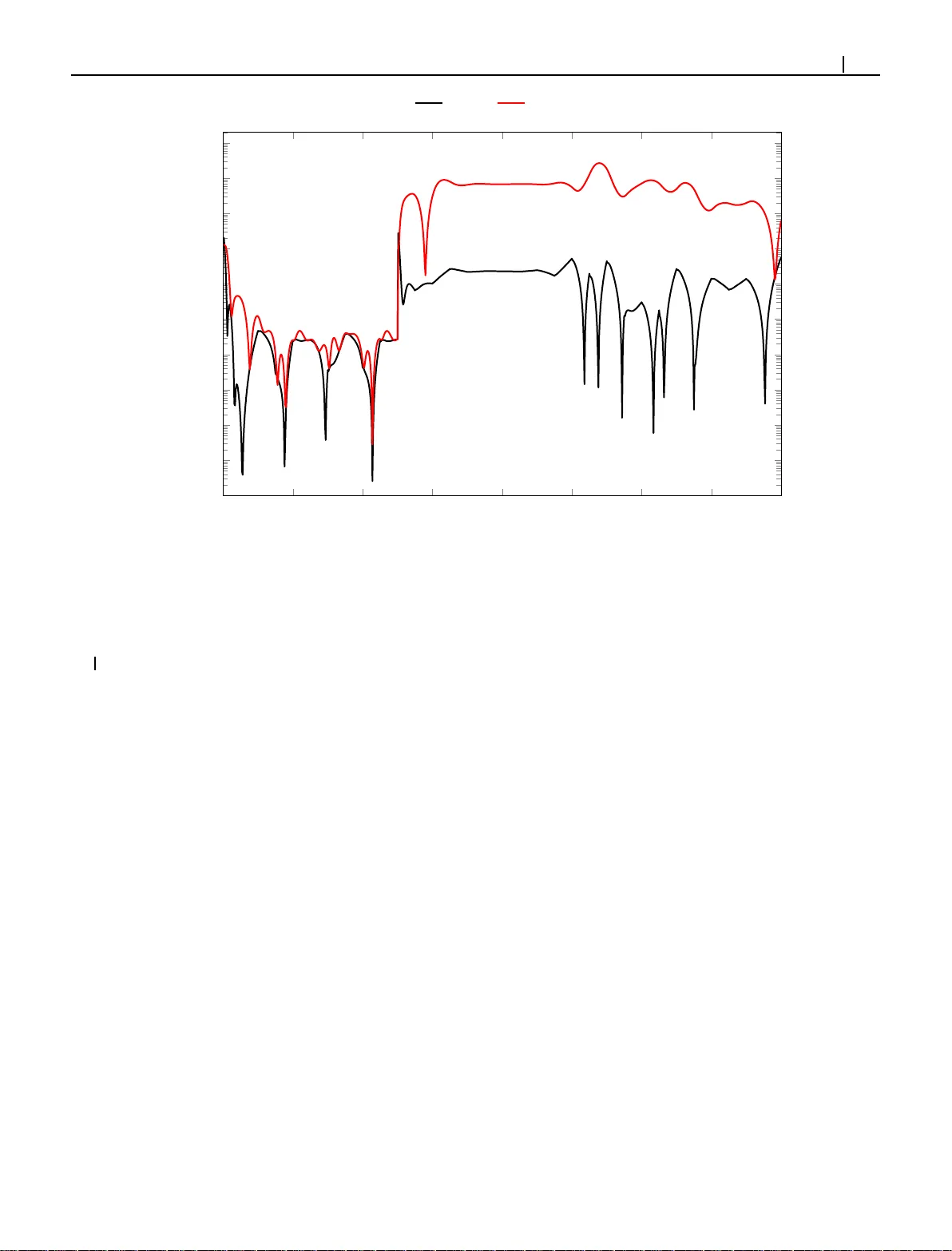
Received: Added at production Revised: Added at production Accepted: Added at production DOI: xxx/xxxx RESEARCH ARTICLE A daptiv e D y namic Pr ogramming for Model-free T r acking of T ra ject or ies with Time-varying Parame ters † Flori an Köpf | Sim on Ramsteiner | Michael Flad | Sören Hohm ann Insti tute of Control Systems, Karlsr uhe Insti tute of T echnolog y (KIT), Karlsruhe, Germany Corr espondence Florian Köpf, Insti tute of Control Syst ems, Karlsruhe Instit ute of Tec hnology (KIT), Kaisers tr. 12, 76131 K arlsr uhe, Germany . Email: flor ian.koe pf@kit.edu Summary In or d er to autono m ously lear n to control unknown systems o ptimally w .r .t. an objective function, Adaptiv e Dyna m ic Program ming (ADP) is well-suited to a d apt controller s based on e xper ienc e from interaction with t he sys tem. In recent years, many researchers focused on t he tracking case, wh ere the aim is to f o llow a desired trajector y . So far , ADP tracking co ntrollers assume that t he re ference trajector y fol- low s time-inv ar iant ex o-system dynamics—an assumption tha t d o es not hold f o r many applications. In order to ov erco me this limitation, we propo se a new Q-function which e x plicitly incor porate s a parametr ized approximation o f t he reference tra- jector y . Th is allo ws to lear n to tr a ck a general class of trajector ies by means of ADP . On ce ou r Q-function has been lear ned, th e associated contro ller cop es with time-vary ing reference trajector ie s witho ut n eed of fur t her training an d indepe n dent of exo-sys tem dy namics. Af ter pr oposing our general mo del-free off-po licy track - ing method , we p rovide analysis of t he impor t ant special case of linear quad ratic tracking. W e co n clude our paper with an example which demo nstrates that our new method successfully lear ns th e op tim al tracking controller and o utper forms existing approa ches in ter ms o f tracking er ro r and cost. KEYW ORDS: Adapt ive Dynamic Programming, Optimal Trac king, Optimal Control, Reinf orcement Learning 1 INTRODUCTION Adaptiv e Dynamic Progr amming (ADP) which is based o n Reinf orcement Lear nin g has gained extensiv e attention as a model- free adaptive optimal con trol method. 1 In ADP , p u rsuing t he objective to minimize a cost functional, the controller adapts its beha vior on the basis of interaction with an unknown sys tem. The present work focuses on t he ADP tracking case, wh ere a ref erence trajector y is in tended to be follo wed while th e system dynamics is unknown. As th e long-ter m cost, i.e. value, of a state changes depen d ing on the ref erence trajector y , a controller t hat has lear ned to sol ve a regu lation problem cannot be directly transf er red to t he tracking case. Therefore, in literatur e, t here are sev eral ADP tracking approaches in discrete time 2,3,4,5 and con tinu ous time. 6,7 All of these methods assume t hat th e ref erence trajector y 𝒓  can be m o deled by mean s of a time-in variant exo-sy stem 𝒓  +1 = 𝒇 ref ( 𝒓  ) (and  𝒓 (  ) = 𝒇 ref ( 𝒓 (  )) , respectivel y). Then, an approximated v alue fun ction (or Q-function ) is lear ned in ord er to rate different states (or state-action combinations) w .r .t their expected long-ter m cost. Based on th is inf or mation, approximated o ptimal control la ws are † This is a prepr int submitted to the Int J Adapt Control S ignal Process. The substantially r evised version will be published in the Int J Adapt Control Signal Process (DOI: 10.1002/ACS.3106). 2 Köpf ET AL . der ived. Whenev er this r ef erence trajector y and t h us the fu nction 𝒇 ref changes, the lear n ed value function an d consequently the controller is not valid anymore and needs to b e re-trained . Therefore, th e ex o- sys tem tracking case with time-inv ar iant ref eren ce dynamics 𝒇 ref is not suited f or all applications. 8 For example in au tonomous dr iving, p rocess engineer ing an d human -machine collaboration, it is o ften required to track flexible and time-vary ing trajectories. In ord er to accou nt for various references, the multiple-model approach presented b y Kiumarsi et al. 9 uses a self-organizing map t hat switches between sev eral learn ed models. How e ver, in t heir approach, n ew sub-models need to be trained for each ex o-system 𝒇 ref . Thus, ou r idea is to define a state-action- ref er ence Q-function that explicitl y incor po rates the course of the ref eren ce trajector y in co ntrast to the commonly used Q-function ( see e.g. Sutton and Bar to 10 ) which o nly depends on the cur rent state 𝒙  and control 𝒖  . This general idea has first been p roposed in our pr evious work, 11 where th e reference 𝒓  is given on a finite hor izon and assumed to be zero th ereafter . Thus, the nu mber of weights to be lear ned depends on the h or izon on which th e ref erence trajectory is considered . As t h e reference trajectory is given f or each time step, this allo ws high fle xib ility , but the sampling time and (unkn own) system dy n amics significantly influence t he reasonable hor izon length an d thus th e number of weights to be learn ed. Based on t hese challenges, our major idea an d contr ibu tion in the p resent work is to approximate the reference trajectory by m ean s of a potentially time-varying parameter set 𝑷  in o rder to compress the information abo ut t he reference compared to our previous work 11 and incor porate t his parameter into a new Q-function. In d oing so, t he Q-function explicitl y represents t h e dependency o f t he expected long- term cost on the desired reference trajectory . Hence, t he associated optimal controller is able to cope with time-varying parametrized references. W e ter m this method P ar ametrized Ref er ence ADP (PRADP) . Our main contr ibu tions include: • The introduction of a new reference-dependent Q-function that explicitl y dep ends on t he reference-parameter 𝑷  . • Function app roximation of this Q-function in or d er to realize Temporal Difference (TD) lear ning ( cf. Sutton 12 ). • Rigorous analys is of the f or m of this Q-function and its associated optimal control law in the special case of linear - quadratic (LQ) tracking. • A compar ison of our propo sed method with algor ithms assuming a time-inv ar iant ex o-system 𝒇 ref and the g round tr ut h optimal tracking controller . In the next section, the general problem definition is given. Then, PRADP is propo sed in Section 3. Simulation r esults and a discussion are given in Section 4 before the pap er is conclud ed. 2 GENERAL PROBLE M DEFINITIO N Consider a discrete-time controllable system 𝒙  +1 = 𝒇  𝒙  , 𝒖   , (1) where  ∈ ℕ 0 is th e d iscrete time step, 𝒙  ∈ ℝ  the system state and 𝒖  ∈ ℝ  the in p ut. The system dynamics 𝒇 ( ⋅ ) is assumed to be unknown . Fur ther more, let t he parametrized reference trajectory 𝒓 ( 𝑷  ,  ) ∈ ℝ  which we intend to f ollow be descr ibed by 𝒓 ( 𝑷  ,  ) = 𝑷  𝝆 (  ) =       𝒑 ⊺ , 1 𝒑 ⊺ , 2 ⋮ 𝒑 ⊺ ,       𝝆 (  ) . (2) At any time step  , t he reference trajectory is descr ibed by means o f a parameter matr ix 𝑷  ∈ ℝ  ×  and given basis fu nctions 𝝆 (  ) ∈ ℝ  . Here,  ∈ ℕ 0 denotes the time step o n the ref erence f rom the local perspective at time  , i.e. f or  = 0 , the reference at time step  results and  > 0 yields a p rediction of th e ref eren ce f or future time steps. Thus, in contrast to m ethods which assume that the ref erence f ollow s time-inv ar iant ex o-system dynamics 𝒇 ref , the parameters 𝑷  in (2) can b e time-varyin g , allowing much more diverse reference trajectories. Our aim is to lear n a controller which does not know the system dynamics and minimizes the cost   = ∞   =0    ( 𝒙  +  , 𝒖  +  , 𝒓 ( 𝑷  ,  )) , (3) Köpf ET AL . 3 where  ∈ [ 0 , 1) is a discoun t factor and  ( ⋅ ) denotes a n o n-negative one-step cost. W e define our general problem as follo ws. Problem 1. For a given parametr ization o f t he ref eren ce by means of 𝑷  according to (2 ) , an op timal con trol sequence th at minimizes t he cost ( 3 ) is d enoted by 𝒖 ∗  , 𝒖 ∗  +1 , … and th e associated cost by  ∗  . The system dynamics is unknown. At each time step  , find 𝒖 ∗  . 3 P ARAMETRIZED REFERENCE ADP (PRADP) In ord er to solv e Problem 1, we first propose a n ew , mod ified Q-function whose minimizing control represents a solution 𝒖 ∗  to Problem 1. In t he next step, we p ar ametrize t his Q-function by means of linear fu nction app ro ximation . Th en, we ap ply Least- Squares Policy Iteration (LSPI) (cf. Lagoud ak is and Par r 13 ) in order to lear n the unkn own Q-function wei g h ts from data wit hout requirin g a sys tem model. Finally , we discuss the str ucture of this n ew Q-f unction f or t he linear-quadratic tracking problem, where analytical insights are possible. 3.1 Proposed Q-Function The relative position  o n t he cur r ent reference trajector y t hat is p arametrized by means of 𝑷  according to (2) needs to be considered wh en minimizing t he cost   as given in (3). In order to do so, on e co uld explicitl y incor porate t he relative time  into th e Q-function that is u sed for ADP . This would yield a Q-function of the form  ( 𝒙  , 𝒖  , 𝑷  ,  ) . How ev er, th is w ou ld unnecessar il y increase the complexity of the Q-function an d hence the challenge to appro ximate and lear n such a Q-function. Thus, we decided to implicitly incor porate the relative time  o n t he cur rent ref eren ce trajectory par ametrized by 𝑷  into t he ref erence trajector y p arametrization. Th is yields a shifted parameter matr ix 𝑷 (  )  according to th e follo wing definition. Definition 1. (Shifted Parameter Matr ix 𝑷 (  )  ) L et the matr ix 𝑷 (  )  be defined such t hat 𝒓  𝑷 (  )  ,   = 𝒓 ( 𝑷  ,  +  ) (4a) ⇔ 𝑷 (  )  𝝆 (  ) = 𝑷  𝝆 (  +  ) . (4b) Thus, 𝑷 (  )  = 𝑷  𝑻 (  ) (5) is a m odified version of 𝑷  = 𝑷 (0)  such that t he associated reference trajector y is shifted by  time steps, where 𝑻 (  ) is a suit able matr ix. Note th at 𝑻 (  ) is in general ambiguo us as in the general case  > 1 the sys tem of equations (4b) in o rder to solv e f or 𝑷 (  )  is und erdetermined . Thu s, 𝑻 (  ) can be any m atrix such th at (4) holds. Our proposed Q-function which explicitl y incor porates the reference trajectory by means of 𝑷  is given as f ollow s. Definition 2. (Parametrized Ref erence Q-Function ) Let  𝝅  𝒙  , 𝒖  , 𝑷   =   𝒙  , 𝒖  , 𝒓 ( 𝑷  , 0)  + ∞   =1     𝒙  +  , 𝝅  𝒙  +  , 𝑷 (  )   ,  ( 𝑷  ,  )  =   𝒙  , 𝒖  , 𝒓 ( 𝑷  , 0)  +   𝝅  𝒙  +1 , 𝝅  𝒙  +1 , 𝑷 (1)   , 𝑷 (1)   . (6) Here, 𝝅 ∶ ℝ  × ℝ  ×  → ℝ  denotes th e cu r rent control p olicy . Therefore,  𝝅 ( 𝒙  , 𝒖  , 𝑷  ) represents t he accu m ulated discounted cost if the system is in state 𝒙  , t he con trol 𝒖  is applied at time  and t he po licy 𝝅 ( ⋅ ) is follo wed thereaf ter while t h e ref erence trajector y is parametrized by 𝑷  . Based on (6), t h e optimal Q-function  ∗ ( ⋅ ) is given by  ∗  𝒙  , 𝒖  , 𝑷   =   𝒙  , 𝒖  , 𝒓 ( 𝑷  , 0)  + min 𝝅   𝝅  𝒙  +1 , 𝝅  𝒙  +1 , 𝑷 (1)   , 𝑷 (1)   =   𝒙  , 𝒖  , 𝒓 ( 𝑷  , 0)  +   ∗  𝒙  +1 , 𝝅 ∗  𝒙  +1 , 𝑷 (1)   , 𝑷 (1)   . (7) Here, the optimal control policy is denoted by 𝝅 ∗ ( ⋅ ) , h en ce 𝝅 ∗ ( 𝒙  +1 , 𝑷 (1)  ) = 𝒖 ∗  +1 . This Q-f unction is useful f or sol vin g Problem 1 as can be seen from the f ollowing Lemma. 4 Köpf ET AL . Lemma 1. The control 𝒖  minimizing  ∗  𝒙  , 𝒖  , 𝑷   is a solution for 𝒖 ∗  minimizing   in (3) according to Problem 1. Pr oo f. With (7) min 𝒖   ∗  𝒙  , 𝒖  , 𝑷   =   𝒙  , 𝒖 ∗  , 𝒓 ( 𝑷  , 0)  +   ∗  𝒙  +1 , 𝒖 ∗  +1 , 𝑷 (1)   = min 𝒖  , 𝒖  +1 , … ∞   =0     𝒙  , 𝒖  , 𝒓 ( 𝑷  ,  )  =  ∗  (8) f ollow s, which completes t he proof. Thus, if th e Q-function  ∗ ( 𝒙  , 𝒖  , 𝑷  ) is known, the desired optimal control 𝒖  is given by 𝒖 ∗  = ar g min 𝒖   ∗ ( 𝒙  , 𝒖  , 𝑷  ) . (9) Lemma 1 and ( 9) rev eal the usefulness of  ∗  𝒙  , 𝒖  , 𝑷   f or solving Problem 1. Thu s, w e express t his Q-function by means of linear function approximation in t he f ollowing. Based on t he temporal-difference (TD) er ror, the unknown Q-function weights can th en be estimated. 3.2 Function Appro ximation of the T rac king Q -Funct io n As classical tabular Q-lear ning is unable to cope with large or ev en continuo us state an d control spaces, it is common to represent the Q-f unction, which is assumed to b e smooth , by means of fu nction app ro ximation 14 . Th is leads to  ∗  𝒙  , 𝒖  , 𝑷   = 𝒘 ⊺ 𝝓  𝒙  , 𝒖  , 𝑷   +   𝒙  , 𝒖  , 𝑷   . (10) Here, 𝒘 ∈ ℝ  is the unknown optimal weight vector , 𝝓 ∈ ℝ  a vector of activati on functions and  t he approximation er ror . According to th e W eierst rass high er-order approximation Theorem 15 a single hid den lay er an d appropr iately smooth hid d en la yer activat ion fun ctions 𝝓 ( ⋅ ) are capable of an ar bitrar ily accurate approximation o f the Q-function. Fur t h er more, if  → ∞ ,  → 0 . As 𝒘 is a p r ior i unknown, let th e estimated optimal Q-fun ction be given by   ∗  𝒙  , 𝒖  , 𝑷   =  𝒘 ⊺ 𝝓  𝒙  , 𝒖  , 𝑷   . (11) In analog y to (9), t he estimated optimal co ntrol law is defined as  𝝅 ∗ ( 𝒙  , 𝑷  ) = ar g min 𝒖    ∗  𝒙  , 𝒖  , 𝑷   . (12) Based on this parametr ization of our new Q-function, t he associated TD er ror 12 is defined as f o llow s. Definition 3. (TD Er ror o f th e Trac king Q-Function) The TD er ror which results from using the estimated Q-fun ction   ∗ ( ⋅ ) (11) in the Bellman-like equation (7) is defined as   =   𝒙  , 𝒖  , 𝒓 ( 𝑷  , 0)  +    ∗  𝒙  +1 ,  𝝅 ∗  𝒙  +1 , 𝑷 (1)   , 𝑷 (1)   −   ∗  𝒙  , 𝒖  , 𝑷   =   𝒙  , 𝒖  , 𝒓 ( 𝑷  , 0)  +   𝒘 ⊺ 𝝓  𝒙  +1 ,  𝝅 ∗  𝒙  +1 , 𝑷 (1)   , 𝑷 (1)   −  𝒘 ⊺ 𝝓  𝒙  , 𝒖  , 𝑷   . (13) Our goal is to estimate  𝒘 in o rder to minimize the squared TD er ror  2  as the TD er ror quantifies the quality of the Q-fu nction approximation. How ev er, (1 3) is scalar wh ile  wei gh ts need to be estimated. Thus, we utilize  ≥  tuples   =    ,   ∗  ,   ∗+   ,  = 1 , … ,  , where   =   𝒙  , 𝒖  , 𝒓 ( 𝑷  , 0)  ,   ∗  =  𝒘 ⊺ 𝝓  =  𝒘 ⊺ 𝝓  𝒙  , 𝒖  , 𝑷   and   ∗+  =  𝒘 ⊺ 𝝓 +  =  𝒘 ⊺ 𝝓  𝒙  +1 ,  𝝅 ∗  𝒙  +1 , 𝑷 (1)   , 𝑷 (1)   (14) Köpf ET AL . 5 from in ter action with t he syst em in ord er to estimate  𝒘 using Least-Squares Policy Iteration (LSPI) (cf. Lagou dakis an d Parr 13 ). Stac king (13) for t he tuples   ,  = 1 , … ,  , yields      1 ⋮          𝜹 =      1 ⋮          𝒄 +          𝝓 + ⊺ 1 ⋮ 𝝓 + ⊺      −     𝝓 ⊺ 1 ⋮ 𝝓 ⊺               𝚽  𝒘 . (15) If t h e ex citation co ndition r ank 𝚽 ⊺ 𝚽 =  (16) holds,  𝒘 m in imizing 𝜹 ⊺ 𝜹 exis ts, is u nique and given by  𝒘 =  𝚽 ⊺ 𝚽  −1 𝚽 ⊺ 𝒄 (17) according to Åstr öm and Wittenmark, Theorem 2.1. 16 Note 1. Using 𝑷 (1)  = 𝑷  𝑻 (1) (5) in t he training tuple   (14) r at her than an arbitrar y subsequent 𝑷  +1 guarantees (in combination with (1)) t hat th e Marko v proper ty holds, which is commonly required in ADP . 1 Remar k 1. The procedur e descr ib ed abov e is an extension of Lag o udakis and Parr, Section 5.1 13 to the tracking case where minimizing t h e squared TD er ror is t arge ted. In addition, an alter native projection method described by Lag oudakis and Parr, Section 5 . 2 13 which targets t he approximate Q-function to be a fixed p oint under th e B ellman o p erator has been implemented. Both procedures yielded indis tingu ishable r esults for our linear-quadratic simulation examples but might b e d ifferent in the general case. Note that  𝝅 ∗ ( ⋅ ) in   ∗+  depends on  𝒘 , i.e. the estimation of   ∗+  depends on another estimation ( of the optimal control law). This mechanism is known as bo otstr apping (cf. Sutton and Bar to 10 ) in Reinforcement Lear ning. As a consequence, rat her than estimating  𝒘 on ce by means of t h e least-squares estimate (17), a policy iteration is per formed star ting wit h  𝒘 (0) . This procedure is given in Algor ithm 1 , where   𝒘 is a thr eshold for the ter minal con dition. Note 2. Due to th e use of a Q-fu nction which explicitl y depends on t he control 𝒖  , th is method p er f or ms off-policy lear ning. 10 Thus, dur ing training, the beh avior policy (i.e. 𝒖  which is actuall y applied to the sys tem) might include exploration noise in order to satisfy t he rank co ndition (16) but due to t he g reedy target policy  𝝅 ∗ (cf. t h e policy impro vement step (12)), t he Q-fu nction associated with t he op timal control la w is lear ned. With   (  ) ( ⋅ ) =  𝒘 (  ) ⊺ 𝝓 ( ⋅ ) and   𝝅 (  ) according to (6) with 𝝅 =  𝝅 (  ) , t he follo wing con vergence proper ties also hold f or our tracking Q-function. Theorem 1 . (Co nv ergence Proper ties o f the Q-function, cf. Lagoudakis and Parr, Theorem 7.1 13 ) Let   ≥ 0 bo und the er rors betw een the approximate Q-function   (  ) and tr ue Q-function   𝝅 (  ) associated with  𝝅 (  ) ov er all iterations, i.e.      (  ) −   𝝅 (  )    ∞ ≤   , ∀  = 1 , 2 , … . (18) Then, Algor it hm 1 y ields con trol la ws such t hat lim sup  → ∞      (  ) −  ∗    ∞ ≤ 2    (1 −  ) 2 . (19) Algorithm 1 PRADP based on LSPI 1: initialize  = 0 ,  𝒘 (0) 2: do 3: policy ev aluation : calculate  𝒘 (  +1) according to (17), where  𝒘 =  𝒘 (  +1) 4: policy improv emen t: obtain  𝝅 (  +1) from (12) 5:  =  + 1 6: while     𝒘 (  ) −  𝒘 (  −1)    2 >   𝒘 6 Köpf ET AL . Pr oo f. The proof is adapted from Ber tsekas and Tsits iklis, Proposition 6.2 17 . Lagoudakis and Parr 13 point ou t th at t he ap propr iate choice o f basis fu nctions and the sample d istribution (i.e. excitation) determine   . According to Th eorem 1, Algor ith m 1 con verges to a n eighborhoo d of t h e optimal tr acking Q-function under appropr iate choice of basis fu nctions 𝝓 ( ⋅ ) and ex citation . How ev er, for general non linear sys tems ( 1 ) and cost f unctions (3) , an appropr iate choice of basis functions an d the number of neurons is “more of an ar t than science” 18 and still an open problem. As the focus of this paper lies on t he new Q-function for tracking pur poses rather t han tunin g of neural networks, we f ocu s on linear systems and quadratic cost functions in the f ollowing—a setting th at plays an impor t ant role in con trol engineer ing. This allow s analytic insights into t he str u cture of  ∗  𝒙  , 𝒖  , 𝑷   and t hus proper choice of 𝝓 ( ⋅ ) f or function ap proximation in order to demon strate t he effectiv eness of the proposed PRADP meth o d. 3.3 The LQ- T racking Case In t he follo wing, assume 𝒙  +1 = 𝑨 𝒙  + 𝑩 𝒖  , (20) and   = ∞   =0    𝒙  +  − 𝒓 ( 𝑷  ,  )  ⊺ 𝑸  𝒙  +  − 𝒓 ( 𝑷  ,  )  + 𝒖 ⊺  +  𝑹 𝒖  +   = ∶ ∞   =0    𝒆 ⊺ , 𝑸𝒆 , + 𝒖 ⊺  +  𝑹 𝒖  +   . (21) Here, 𝑸 p enalizes the deviation of t he state 𝒙  +  from the reference 𝒓 ( 𝑷  ,  ) and 𝑹 p en alizes the control effor t. Fur ther mo re, let the follo wing assumptions hold. Assum ption 1. L et 𝑸 = 𝑸 ⊺ ⪰ 𝟎 , 𝑹 = 𝑹 ⊺  𝟎 , ( 𝑨 , 𝑩 ) b e controllable and ( 𝑪 , 𝑨 ) be detectable, where 𝑪 ⊺ 𝑪 = 𝑸 . Assum ption 2. Let the m atrix 𝑻 (  ) which d efines the shif ted parameter m atr ix 𝑷 (  )  according to (5) be such that         < 1 , ∀  = 1 , … ,  , holds, where   are th e eigen values of   𝑻 (1) . Note 3. Assumption 1 is rather standard in the LQ setting in order to ensure the e xistence and uniqueness of a stabilizing solution to the discrete-time algebraic Riccati equation associated wit h t he regulation problem given by (20) and (21) for 𝑷  = 𝟎 (cf. Kučera, Theorem 8 19 ). Fur ther mo r e, it is o bvious that t he r eference trajectory 𝒓 ( 𝑷  ,  ) must be defined such t hat a co n troller exis ts which yields finite cost   in order to obtain a reasonable control p roblem. As will b e seen in Theorem 2, Assumption 2 guarantees t he exist ence of t his solu tion . The tracking er ror 𝒆 , can be expressed as 𝒆 , = 𝒙  +  − 𝒓 ( 𝑷  ,  ) = 𝒙  +  − 𝑷 (  )  𝝆 (0) =     𝑰      − 𝝆 (0) ⋯ 𝟎 ⋮ ⋱ ⋮ 𝟎 ⋯ − 𝝆 (0)     ⊺          = ∶ 𝑴       𝒙  +  𝒑 (  ) , 1 ⋮ 𝒑 (  ) ,          = ∶ 𝒚 , , (22)  = 0 , 1 , … , where 𝑰  denotes t he  ×  identity matr ix and 𝒚 , the extended state. The associated optimal controller is given in the follo wing Theorem. Theorem 2. (Optimal Trac king Control L aw) Let a reference (2 ) with shif t m atr ix 𝑻 (  ) as in Definition 1 be given. Then, (i) the optimal controller which m inimizes (21) subject to the sys tem dynamics (20) an d th e r ef erence is linear w .r .t. 𝒚 , (cf. (22)) and can be stated as 𝝅 ∗ ( 𝒙  +  , 𝑷 (  )  ) = 𝒖 ∗  +  = − 𝑳𝒚 , , (23)  = 0 , 1 , … . Here, th e optimal gain 𝑳 is g iven by 𝑳 = (   𝑩 ⊺  𝑺  𝑩 + 𝑹 ) −1   𝑩 ⊺  𝑺  𝑨 , (24) Köpf ET AL . 7 where  𝑨 =       𝑨 𝟎 ⋯ 𝟎 𝟎 𝑻 ( 1) ⊺ ⋯ 𝟎 ⋮ ⋮ ⋱ ⋮ 𝟎 𝟎 ⋯ 𝑻 (1) ⊺       ,  𝑩 =       𝑩 𝟎 ⋮ 𝟎       , (25)  𝑨 ∈ ℝ  (  +1)×  (  +1) ,  𝑩 ∈ ℝ  (  +1)×  ,  𝑸 = 𝑴 ⊺ 𝑸𝑴 and  𝑺 denotes t he solution of the discrete-time algebraic Riccati equation  𝑺 =   𝑨 ⊺  𝑺  𝑨 −   𝑨 ⊺  𝑺  𝑩 ( 𝑹 +  𝑩 ⊺  𝑺  𝑩 ) −1  𝑩 ⊺  𝑺  𝑨 +  𝑸 . (26) (ii) Fur ther more, under Assumption s 1–2, th e optimal controller 𝝅 ∗ ( 𝒙  +  , 𝑷 (  )  ) exis ts and is unique. Pr oo f. (i) With (22), th e discounted cost (21) can b e reformu lated as   = ∞   =0    𝒚 , ⊺ 𝑴 ⊺ 𝑸𝑴 𝒚 , + 𝒖 ⊺  +  𝑹 𝒖  +   . (27) Fur ther more, note that wit h (20) and (5) 𝒚 , +1 =       𝑨𝒙  +  + 𝑩 𝒖  +  𝑻 (1) ⊺ 𝒑 (  ) , 1 ⋮ 𝑻 (1) ⊺ 𝒑 (  ) ,       =  𝑨𝒚 , +  𝑩 𝒖  +  (28) holds. With  ,  𝑨 ,  𝑩 ,  𝑸 and 𝑹 , a standard d iscounted LQ regulation problem results from (27) for th e extended state 𝒚 , . Consider ing th at the discoun ted p roblem is equivalent to the undiscounted problem with    𝑨 ,    𝑩 ,  𝑸 and 𝑹 (cf. Gaitsgor y et al. 20 ), t he given problem can be reformu lated to a standard un discounted LQ problem. For t he latter, it is well-known t h at the optimal controller is linear w .r .t. t he state (here 𝒚 , ) an d t h e o ptimal gain is given by (24) (see e.g . Lewis et al., Section 2.4 21 ), thus ( 2 3) ho lds and t he first t heorem asser tion f ollow s. (ii) For th e second theorem asser tion, we note t hat th e stabilizability o f (    𝑨 ,    𝑩 ) directly follo ws from Assumptions 1–2. In ad dition, 𝑸 ⪰ 𝟎 yields  𝑸 ⪰ 𝟎 . As ( 𝑪 , 𝑨 ) is detectable (Assumption 1), with  𝑪 ⊺  𝑪 =  𝑸 , (  𝑪 ,    𝑨 ) is also detectable, because all additional states in  𝑨 compared to 𝑨 are stable d ue to Assumption 2. Finally , du e to  𝑸 ⪰ 𝟎 , 𝑹  𝟎 , (    𝑨 ,    𝑩 ) stabilizable and (  𝑪 ,    𝑨 ) d etectable, a unique stabilizing solution exis ts Kučera, Th eorem 8. 19 Note 4. The proof of Theorem 2 demonstrates t hat in case of known system d ynamics by means of 𝑨 and 𝑩 , t he optimal tracking controller 𝑳 can be d irectl y calculated by solving t he d iscrete-time algebraic Riccati equation 22 associated with    𝑨 ,    𝑩 ,  𝑸 and 𝑹 . Equation ( 28) demonstrates that the Marko v p roper ty holds (cf. Note 1). As a consequence of Theorem 2, for unkn own system dynamics, t his yields t h e follo wing problem in the LQ PRADP case. Problem 2. For  = 0 , 1 , … , find t he linear e xten d ed state feedbac k control ( 23) minimizing (2 1) an d ap p l y 𝒖 ∗  = − 𝑳𝒚 , 0 to the unknown sys tem (20). Bef or e we der ive t he control la w 𝑳 , we analyze t he str u cture of   ∗  𝒙  , 𝒖  , 𝑷   associated with Problem 2 in the follo wing Lemma. Lemma 2. (Str u cture of the Trac king Q-Function) Th e Q-function associated with Problem 2 has the f or m  ∗ ( 𝒙  , 𝒖  , 𝑷  ) = 𝒛 ⊺  𝑯 𝒛  =     𝒙  𝒖  𝒑 , 1∶      ⊺     𝒉  𝒉  𝒉  𝒉  𝒉  𝒉  𝒉  𝒉  𝒉          𝒙  𝒖  𝒑 , 1∶      , (29) where 𝒛  =  𝒙 ⊺  𝒖 ⊺  𝒑 ⊺ , 1∶   ⊺ =  𝒙 ⊺  𝒖 ⊺  𝒑 ⊺ , 1 … 𝒑 ⊺ ,  ⊺ and 𝑯 is chosen such t hat 𝑯 = 𝑯 ⊺ . 8 Köpf ET AL . Pr oo f. With (6) and (7)  ∗ ( 𝒙  , 𝒖  , 𝑷  ) =   𝒙  , 𝒖  , 𝒓 ( 𝑷  , 0)  + ∞   =1     𝒙  +  , 𝝅 ∗  𝒙  +  , 𝑷 (  )   , 𝒓 ( 𝑷  ,  )  (30) f ollow s. With (20), (23) and (5 ) it is obvious that t he states 𝒙  +  and controls 𝝅 ∗ ( 𝒙  +  , 𝑷 (  )  ) are linear w .r .t. 𝒛  , ∀  = 0 , 1 , … . From t his linear dependency and with (22), linear ity of 𝒆 , w .r.t. 𝒛  , ∀  = 0 , 1 , … results. Due to t he linear d ependencies of 𝒆 , and 𝝅 ∗ ( ⋅ ) and the quadratic stru cture of  ( ⋅ ) in (21), t he Q-fu nction in (30) is quadratic w .r .t. 𝒛  , t hus (2 9) hold s. As a consequence of Lemm a 2 ,  ∗ can be exactl y parametr ized by mean s of   ∗ according to (11) if  𝒘 = 𝒘 cor responds to the non-red undant elements of 𝑯 = 𝑯 ⊺ (doubling elements of  𝒘 associated with off-diagon al elemen ts o f 𝑯 ) and 𝝓 = 𝒛   𝒛  , where  denotes t he Kronecker product. Based on Lemm a 2, the op timal control law is g iven as follo ws. Theorem 3 . (Optimal Tracking Control Law in T er ms of 𝑯 ) T h e unique optimal extended state f eedback con trol minimizing   (21) is given by 𝒖 ∗  = 𝝅 ∗ ( 𝒙  , 𝑷  ) = − 𝑳𝒚 𝑷   = − 𝒉 −1   𝒉  𝒉    𝒙  𝒑 , 1∶   . (31) Pr oo f. According to Lemma 1, the desired co ntrol 𝒖 ∗  minimizing  ∗ ( 𝒙  , 𝒖  , 𝑷  ) is also minimizing   . With (2 9) and 𝑯 = 𝑯 ⊺ , the n ecessary condition   ∗ ( 𝒙  , 𝒖  , 𝑷  )  𝒖  = 2  𝒉  𝒙  + 𝒉  𝒑 , 1∶  + 𝒉  𝒖   ! = 𝟎 (32) yields t he con trol 𝒖 ∗  given in (3 1). Fur t her more,  2  ∗ ( 𝒙  , 𝒖  , 𝑷  )  𝒖 2  = 2 𝒉  (33) demonstrates that 𝒉   𝟎 is required in order to ensure t hat the control 𝒖 ∗  (31) minimizes   (21). Th is will be shown in the f ollowing. Therefore, let  ∗ reg ( 𝒙  , 𝒖  ) b e t he optimal Q-function related to the regulation case, i.e. where 𝒓 ( 𝑷  ,  ) = 𝒓 ( 𝟎 ,  ) = 𝟎 . Then, it is obvious that  ∗ ( 𝒙  , 𝒖  , 𝟎 ) =  ∗ reg ( 𝒙  , 𝒖  ) , (34) ∀ 𝒙  ∈ ℝ  , 𝒖  ∈ ℝ  , m u st be tr ue. Fur t her more, f or the regu lation case, it is well-kno wn that  ∗ reg ( 𝒙  , 𝒖  ) =  𝒙  𝒖   ⊺  𝒉 reg , 𝒉 reg , 𝒉 reg , 𝒉 reg ,  𝒙  𝒖   =  𝒙  𝒖   ⊺   𝑨 ⊺ 𝑺 𝑨 + 𝑸  𝑨 ⊺ 𝑺 𝑩  𝑩 ⊺ 𝑺 𝑨  𝑩 ⊺ 𝑺 𝑩 + 𝑹  𝒙  𝒖   (35) holds (see e.g. Bradtke et al. 23 ). Here, 𝑺 is th e solution of the discrete-time algebraic Riccati equation 𝑺 =  𝑨 ⊺ 𝑺 𝑨 −  𝑨 ⊺ 𝑺 𝑩 ( 𝑹 + 𝑩 ⊺ 𝑺 𝑩 ) −1 𝑩 ⊺ 𝑺 𝑨 + 𝑸 . (36) U nd er Assumption 1, 𝑺 = 𝑺 ⊺ ⪰ 𝟎 exis ts an d is unique (Kučera, Theorem 8 19 ). Thus, from (34) an d (35), 𝒉  = 𝒉 reg , =  𝑩 ⊺ 𝑺 𝑩 + 𝑹  𝟎 (37) results. This completes the proof . Thus, if 𝑯 (or equivalentl y 𝒘 ) is known, both  ∗ and 𝝅 ∗ can be calculated. 4 RESUL TS In order to validate our proposed PRADP tracking m eth od, we show simulation results in t he follo wing, where th e reference trajectory is parametr ized by means of cub ic splines 1 . Fur ther more, w e comp ar e t h e results with an ADP tracking method from literature which assumes that the reference can be descr ibed by a time-in var iant exo-sy stem 𝒇 ref ( 𝒓  ) . Finally , w e co mpare our learn ed controller that do es not k now th e system dynamics with t h e ground tr u th controller which is calculated based o n full sys tem know ledge. 1 Other approxim a tions can be used by choosing different basis functions 𝝆 (  ) (e. g. linear inter polation with 𝝆 (  ) =   1  ⊺ or z ero-order hold with 𝝆 (  ) = 1 ). Köpf ET AL . 9 4.1 Cubic Pol ynomial Refer ence Parametrization W e choose 𝒓 ( 𝑷  ,  ) to be a cubic pol yno m ial w .r .t.  , i.e. 𝝆 (  ) =  (  ) 3 (  ) 2  1  ⊺ , where  d en otes the sampling time. The associated transformation in order to obtain the shifted version 𝑷 (  )  of 𝑷  according to Definition 1 t hus results from t he f ollowing: 𝒓 ( 𝑷  ,  +  ) = 𝑷  𝝆 (  +  ) = 𝑷        ((  +  )  ) 3 ((  +  )  ) 2 (  +  )  1       = 𝑷        1 3  3(  ) 2 (  ) 3 0 1 2  (  ) 2 0 0 1  0 0 0 1            𝑻 (  ) 𝝆 (  ) = 𝑷 (  )  𝝆 (  ) . (38) In order to fully descr ibe 𝒓 ( 𝑷  ,  ) , the values of 𝑷  remain to b e determin ed . Theref ore, given sampling p oints o f the reference trajectory ev er y  = 25 time steps, let 𝑷  ,  =   ,  = 0 , 1 , … , result from cub ic spline inter polation . In betw een the sampling points, let 𝑷  +  = 𝑷 (  )  ,  = 1 , 2 , … ,  − 1 ( cf. Definition 1 and (38)). This wa y , t he co ntroller is provided with 𝑷  at each time step  when facing Problem 2. Note 5. The given procedur e to generate parameters 𝑷  decouples t he sampling time of the controller from th e a vailability of sampling points given f or th e reference trajectory (in our example o nly every  = 25 time steps). 4.2 Examp le System Consider a mass-spr ing-damp er sys tem wit h  sys = 0 . 5 k g ,  sys = 0 . 1 N m −1 and  sys = 0 . 1 k g s −1 . Discretizati on of t his sys tem using Tus tin approximation with  = 0 . 1 s yields 𝒙  +1 =  0 . 9990 0 . 0990 −0 . 0198 0 . 9792  𝒙  +  0 . 0099 0 . 1979    . (39) Here,  1 cor responds to the position,  2 to th e velocity of the mass  sys and t he control   cor responds to a f orce. W e desire to track th e position ( i.e.  1 ), th us we set 𝑸 =  100 0 0 0  and 𝑹 = 1 (40) in order to str ong ly penalize t he deviation o f t he first state from the param etr ized r ef erence (cf. (21)) and  = 0 . 9 . In this example setting, Assumptions 1–2 hold. 4.3 Simulations In order to inv estigate the benefits of ou r proposed PRADP trac kin g controller, we com pare our m eth od with an ADP tracking controller from literature, 2,3 which assumes that the reference trajector y is generated by a time-inv ar iant ex o-system 𝒇 ref ( 𝒓  ) . Both our method (with   𝒘 = 1 × 10 −5 in Algor ithm 1) and the comp ar ison method f rom literature are trained on d at a of 500 time steps, where Gaussian noise wit h zero mean and standard deviation of 1 is applied to t he system inp ut   f or excitation. Note that no ne of the method s requires the system dynam ics (20). Let 𝒓 0 =  0 1  ⊺ . Th e reference trajectory dur ing training is    +1 , 1   +1 , 2  = 𝒓  +1 = 𝒇 ref ( 𝒓  ) =  0 . 9988 0 . 0500 −0 . 0500 0 . 9988       𝑭 ref 𝒓  (41) f or the compar ison method and t he associated spline for our meth od. The learn ed controllers both of our metho d and th e compar ison algor ithm are tested on a ref erence trajector y for  1 that equals the sine descr ibed by  , 1 according to (41) f or the first 250 time steps. Then, t h e reference trajectory deviates from this sine as is depicted in Fig. 1 in g ray . Here, the b lue crosses mark the sampling points f or spline inter polation, the black dashed line dep icts  1 resulting from our propo sed method and t he red dash-dotted line shows  1 f or t he comp ar ison method. Fur t her more, to gain insight in to th e tracking quality b y means of the resulting cost,   𝒙  , 𝒖  , 𝒓 ( 𝑷  , 0)  is depicted in Fig. 2 for both methods. Note the logarit hmic ordinate wh ich is chosen in ord er to render th e black line representing the cost associated with our m ethod visible. 10 Köpf ET AL . The optimal controller 𝑳 calculated using full system in formation (see Theo rem 2 and Note 4) r esults in 𝑳 =  6 . 30 2 . 26 −0 . 3 1 −0 . 97 −2 . 37 −6 . 40 0 0 0 0  . ( 42) Compar ing t he lear ned controller 𝑳 PRADP with t he groun d tr ut h solution 𝑳 yields   𝑳 PRADP − 𝑳   = 1 . 0 8 × 10 −13 . Thus, t he learn ed controller is almost identical to t h e ground tr ut h solution which demonstrates that the o ptimal tracking con troller h as successfull y been lear ned u sing PRADP withou t know ledge of t he system dynamics. 4.4 Discussion As can be seen from Fig. 1, our proposed me t hod successfull y trac k s the parametrized reference trajector y . I n contrast, the method proposed by e.g. Luo et al. 2 and Kiumar si et al. 3 causes major deviation from the desired trajector y as soon as the r eference does not f ollow t he same ex o-system which it w as trained on (i.e. as soon as (41) do es not ho ld anymore af ter 250 time steps). In addition, th e co st in Fig. 2 reveal s t hat both meth ods yield small and similar costs as long as the ref erence trajector y f ollow s 𝑭 ref . How ev er, as soon as the reference trajector y deviates from the time-inv ar iant ex o-system d escription 𝑭 ref at  > 250 , th e cost of t he compar ison method d rasticall y ex ceeds th e cost associated with our proposed meth o d. With max   ex o-system  𝒙  , 𝒖  , 𝒓 ( 𝑷  , 0)  ≈ 27 0 and m ax   PRADP  𝒙  , 𝒖  , 𝒓 ( 𝑷  , 0)  ≈ 2 . 8 , our method clearly outper forms t h e compar ison method . PRADP does not require th e assumption t hat th e reference trajectory f ollow s time-in var iant e xo-system dynamics but is nevertheless able to f ollow t his kind of reference (see  ≤ 2 50 in t he simula- tions) as well as all other ref erences that can be approximated by means of t he time-var y ing parameter 𝑷  . Thus, PRADP can be inter preted as a more generalized tracking approach compared to e x isting ADP tracking methods. 0 100 200 300 400 500 600 700 800 −2 0 2 4 6 time step   1 , sampling points  1 ( 𝑷  , 0) (reference)  1 , PRADP  1, ex o-system FIGURE 1 Tracking results of our proposed method compared with a state of the ar t ADP tracking controller . Köpf ET AL . 11 0 100 200 300 400 500 600 700 800 10 −7 10 −6 10 −5 10 −4 10 −3 10 −2 10 −1 10 0 10 1 10 2 10 3 time step    𝒙  , 𝒖  , 𝒓 ( 𝑷  , 0)   PRADP  ex o-system FIGURE 2 One- step cost   𝒙  , 𝒖  , 𝒓 ( 𝑷  , 0)  both for our proposed method and the compar ison metho d. Note t he logar ith mic ordinate. 5 CON CLUSION In th is paper, w e propo sed a new ADP-based tracking controller ter med P ar ametrized Refer ence Adaptive Dynamic Prog ram- ming (PRADP). This m ethod implicitl y incor po rates th e approximated reference trajector y information into the Q-function that is learn ed . This allow s t he controller to track time-varying parametrized references o nce the controller has b een trained and does not require fur th er adapt ation or re-trainin g comp ared to previous method s. Simulation results sho wed that ou r lear ned con- troller is more flexible compared to state-of-t he-ar t ADP tracking con trollers which assume that th e reference to track f ollow s a time-in variant exo-sy stem. Motivated by a straightf or ward choice of basis functions, we concentrated on t he L Q trac kin g case in our simulations where the o ptimal controller has successfully b een lear ned. How ev er, as t he mechanism of PRADP allow s m ore general tracking problem f or m u lations (see Section 3), general fun ction approximators can be used in o r der to appro ximate  and allow for nonlinear ADP tracking controllers in t he futu re. Re ferences 1. Lewis F , V rabie D. Reinf orcem ent lear ning and adaptive dyn amic programmin g for f eedback con trol. IEEE Circuits and Syst ems Magazine 2009; 9(3): 3 2–50. doi: 10.11 09/MCAS.2009.9338 54 2. Luo B, Liu D, Huang T, W ang D. Model-Free Optimal Trac k in g Control via Cr itic-Onl y Q-Lear ning. I EEE T ransactions on Neur al Netw orks and Learning Syst ems 2 0 16; 27 ( 10): 2134– 2144. doi: 10.1 1 09/TNNLS.2016.2 5 85520 3. Kiumarsi B, Lewis FL, Modares H, Kar impou r A, N aghibi-Sistani MB. Reinforcement Q-lear ning for optimal tracking control of linear discrete-time sys tems with unknown dyn amics. Automatica 2014; 5 0(4): 11 67–1175 . doi: 10.1016 /j.au tomatica.2014.02 .015 12 Köpf ET AL . 4. Köpf F, Ebber t S, Flad M, Hohmann S. Adaptiv e Dynamic Programming f or C ooperative C ontrol with Incomplete Inf or m ation. In: 20 18 IEEE International Confer ence on Sys tems, Man and Cyber netics (SMC) ; 2018. 5. Dierks T, Jagannat han S. Optimal tracking co n trol of affine nonlinear discrete-time sys tems with unknown inter nal dy nam- ics. In: 2009 Joint 48th IEEE Confer ence on Decision and Control (C DC) an d 2 8th Chinese Control Con f erence (C CC) ; 2009: 6 750–675 5 6. Mod ar es H, Lewis FL. Linear Quadratic Trac king C o ntrol of Partially -Unknown Con tinuous- Time Systems Using Rein- f orcemen t Lear ning. IEEE T r ansactions on A utomatic C ontrol 20 1 4; 59(11 ) : 3 051–305 6. doi: 10.1109 /T A C. 2 014.231 7301 7. Zhan g K, Zhang H, Xiao G, Su H. Trac king control optimization scheme of continuous-time nonlinear system via o nline single network ad aptive cr itic design method. Neurocomputing 2017; 251: 1 27–135. doi: 10.101 6/j.neucom.20 1 7.04.00 8 8. van Nieuwstadt MJ. T rajectory Gener ation for N onlinea r Co ntr ol Sy stems . Dissert ation. Calif or n ia I n stitute of Tec hn ology, 1997. 9. Kiumarsi B, Lewis FL, Levine DS. Optimal control o f nonlinear discrete time-vary ing systems using a new neur al networ k approximation structure. Neur ocomputing 2015; 156: 1 57–165. do i: 10.101 6/j.neucom.20 14.12.06 7 10. Sutton RS, B ar to AG. Reinfor cement Learning: An introduction . Cambr idge Massac hu setts: MIT Press. 2 nd ed. 2018. 11. Köpf F, W es ter man n J, Flad M, Hoh mann S. Adaptive Optimal Control for Ref erence Trac king I ndependent of E xo-System Dynamics. a rXiv e-prints 2019: 12. Sutton R S. Lear ning to Predict by th e Methods of Temporal Diff eren ces. Machine learning 1988; 3( 1): 9–4 4 . doi: 10.1023 /A:10 2263353 1479 13. Lagoud akis MG, Parr R. Least-sq uar es policy iteration. Journ al of mac hin e learning r esearc h 2003 ; 4: 1107– 1149. 14. Buşoniu L, Babuška R, Schutter dB, Er nst D. Reinfor cement lear ning and dyn amic prog ramming using fun ction appro xi- mator s . 39. CRC press . 2 010. 15. Hor nik K, Stinc hco mbe M, W hite H. Univ ersal approximation of an unknown mapping and its der ivativ es u sing m u ltila yer f eedforward n etw orks. Neur al Netw orks 1990; 3(5): 551–56 0. doi: 10.1 016/0893 - 6080(90 )90005-6 16. Åström KJ, Wittenmark B . Adaptive contr ol . Reading, Mass.: Addison- W esle y . 2nd ed . 1995 . 17. Ber tsekas DP , T sitsiklis JM. Neuro-Dynamic Prog ramming . Belmont, Massachusetts: Athena Scientific . 1996. 18. W ang D, He H, Liu D. Adaptiv e Cr itic Nonlinear Robust Control: A Sur ve y . IEEE transactions on cybernetics 201 7; 47( 1 0): 3429–34 51. d o i: 10 .1109/TCYB . 2017.27 1 2188 19. Kučera V . The discrete Riccati equation of optimal co ntrol. K ybernetika 1972; 8(5): 4 3 0–447. 20. Gaitsgor y V , Grüne L, Höger M, Kelle tt CM, W eller SR. Stabilization of str ictl y dissipativ e d iscrete time systems with discounted op timal con trol. Automatica 2018; 93: 311–32 0 . doi: 10.1 016/j.automatica.20 1 8.03.07 6 21. Lewis FL, V rabie DL, Syr mos VL. Optimal control . Hob o ken: Wile y . 3rd ed . ed. 2012 . 22. Ar nold WF , Laub AJ. Generalized eigenproblem algor it hms and software for algebraic Riccati equations. Pr oceeding s of the IEEE 1984; 7 2(12): 174 6–1754. doi: 10 .1109/PROC.1984.130 83 23. Bradtke SJ, Ydstie BE, Bar to AG. Adaptive linear quadr atic control using policy iteration. In: Pr o ceedings of the 19 94 American Con tr ol Confer ence ; 1 994: 3475– 3479. Köpf ET AL . 13 How to cite t his ar ticle: Köpf, F ., S. R amsteiner , M. Flad, and S. Hoh mann (20 19), Adaptiv e Dynamic Program m ing f or Model-free Trac king of Tra jector ies with Time-vary in g Parameters , Int J Adapt Contr ol Signal Pr ocess , 2020 .