Classification accuracy as a proxy for two sample testing

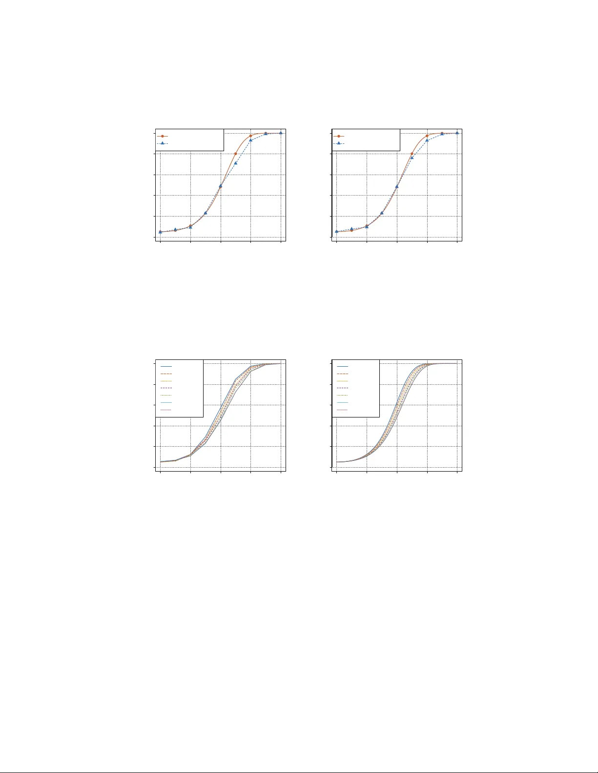
The Annals of Statistics (ac c epted) arXiv: CLASSIFICA TION A CCURACY AS A PR O XY F OR TWO-SAMPLE TESTING By Ilmun Kim , Aadity a Ramd as , Aar ti Singh , and Larr y W asserman Carne gie Mel lon University When data analysts train a classiﬁer and c heck if its accuracy is signiﬁcan tly diﬀeren t from c hance, they are implicitly performing a tw o-sample test. W e inv estigate the statistical prop erties of this ﬂexible approach in the high-dimensional setting. W e pro v e tw o re- sults that hold for all classiﬁers in any dimensions: if its true error remains  -b etter than c hance for some  > 0 as d, n → ∞ , then (a) the p erm utation-based test is consistent (has pow er approac hing to one), (b) a computationally eﬃcient test based on a Gaussian ap- pro ximation of the null distribution is also consisten t. T o get a ﬁner understanding of the rates of consistency , we study a specialized set- ting of distinguishing Gaussians with mean-diﬀerence δ and common (kno wn or unkno wn) co v ariance Σ, when d/n → c ∈ (0 , ∞ ). W e study v ariants of Fisher’s linear discriminan t analysis (LDA) suc h as “naiv e Ba y es” in a nontrivial regime when  → 0 (the Bay es classiﬁer has true accuracy approaching 1/2), and contrast their p o wer with cor- resp onding v ariants of Hotelling’s test. Surprisingly , the expressions for their p o wer match exactly in terms of n, d, δ, Σ, and the LDA ap- proac h is only worse by a constant factor, achieving an asymptotic relativ e eﬃciency (ARE) of 1 / √ π for balanced samples. W e also ex- tend our results to high-dimensional elliptical distributions with ﬁnite kurtosis. Other results of indep enden t interest include minimax low er b ounds, and the optimality of Hotelling’s test when d = o ( n ). Sim u- lation results v alidate our theory , and we present practical tak eaw a y messages along with natural op en problems. 1. In tro duction. The recen t p opularit y of mac hine learning has re- sulted in the extensive teac hing and utilization of prediction metho ds in theoretical and applied communities. When faced with a hypothesis testing problem in practice, data scien tists sometimes opt for a prediction-based test-statistic. W e study one example of this common practice in this paper, concerning arguably the most classical testing and prediction problems — two-sample testing (are the t wo underlying distributions the same?) and classiﬁc ation (learning a classiﬁer that separates the tw o distributions, im- MSC 2010 subje ct classiﬁc ations: Primary 62H15; secondary 62E20 Keywor ds and phr ases: classiﬁcation accuracy, t wo sample testing, high-dimensional asymptotics, Hotelling’s T 2 test, linear discriminant analysis, permutation test 1 imsart-aos ver. 2014/10/16 file: Classification.tex date: February 18, 2020 2 KIM, RAMDAS, SINGH AND W ASSERMAN plicitly assuming they are not the same). Practitioners familiar with machine learning but not the h yp othesis testing literature often ﬁnd it intuitiv e to p erform testing in the follo wing wa y: ﬁrst learn a classiﬁer, and then see if its accuracy is signiﬁcantly diﬀerent from c hance and if it is, then conclude that the distributions are diﬀeren t. The central question that this pap er seeks to answer is “ what ar e the pr os and c ons of the classiﬁer-b ase d appr o ach to two-sample testing? ”. As w e shall detail in Section 2 , the notion of c ost or pric e that is appropriate for the Neyman-Pearson or Fisherian hypothesis testing paradigm, is the p o wer ac hiev able at a ﬁxed false p ositiv e lev el α (in other w ords, the low est possible t yp e-2 error ac hiev able at some presp eciﬁed target type-1 error). Indeed, we approac h this question using the frequen tist p erspective of minimax theory . More formally , w e can restate our question as “ when is the classiﬁer-b ase d test c onsistent, and how do es its p ower c omp ar e to the minimax p ower? ”. 1.1. Pr actic al motivation. Before we delv e into the details, it is worth men tioning that even though this pap er is a theoretical endeav or, the ques- tion was initially practically motiv ated. Many scientiﬁc questions are nat- urally posed as t w o-sample tests — examples abound in epidemiology and neuroscience. As a hypothetical example from the latter, say w e are inter- ested in determining whether a particular brain region resp onds diﬀeren tly under t w o situations (say listening to loud harsh sounds vs soft smo oth sounds), or for a p erson with a medical condition (patient) and a p erson without the condition (control). Often, one collects and analyzes brain data for the same patien t under the t wo contrasting stimuli (to study the eﬀect of change in that stim ulus), or for diﬀerent normal and ill patients under the same stimulus (to study eﬀect of a medical condition). Since the w ork of Golland and Fisc hl ( 2003 ) where the authors examined permutation tests for classiﬁcation with application to neuroimaging analysis, it has b een increas- ingly common in the ﬁeld of neuroscience—see Zhu et al. ( 2008 ); Etzel et al. ( 2009 ); P ereira et al. ( 2009 ); Stelzer et al. ( 2013 )—to assess whether there is a signiﬁcan t diﬀerence b et ween the t wo sets of data collected b y learning a classiﬁer to diﬀerentiate b et w een them (b ecause, for instance, they may b e more familiar with classiﬁcation than tw o- sample testing). Neuroscientists call this st yle of brain deco ding as pattern discrimination and a p ositiv e answ er can b e seen as preliminary evidence that the mental process of in ter- est migh t o ccur within the p ortion of the brain being studied; see Olivetti et al. ( 2012 ) for a discussion of related issues. This classiﬁcation approach to tw o-sample testing has b een considered in other application areas includ- ing genetics ( Y u et al. , 2007 ), sp eec h analysis ( Chen et al. , 2009 ), credit imsart-aos ver. 2014/10/16 file: Classification.tex date: February 18, 2020 CLASSIFICA TION ACCURA CY TEST 3 scoring ( Xiao et al. , 2014 ), ch urn prediction ( Xiao et al. , 2015 ) and video con tent analysis ( Liu et al. , 2018 ). 1.2. Overview of the main r esults. Our ﬁrst contribution is to identify w eak conditions on the classiﬁer that suﬃce for b oth ﬁnite-sample or asymp- totic t yp e-1 error control, as w ell as for asymptotic consistency . • Asymptotic test (Prop osition 9.1 ): W e identify mild conditions under whic h the sample-splitting error of a general classiﬁer ( 2.4 ) is asymptotically Gaussian as n, d → ∞ . W e introduce a test based on this Gaussian approximation and prov e its asymptotic type-1 error con trol. W e also prov e that a suﬃcien t condition for its consistency (for its p o wer to approach one) is that its true accuracy conv erges to 1 / 2 +  for any constant  > 0 as n, d → ∞ at any relativ e rate. • P ermutation test (Theorem 9.1 ): In addition to the asymptotic approac h, we consider t wo types of random p erm utation pro cedures that yield a v alid lev el α test in ﬁnite-sample scenarios. Under the same conditions made before, w e ﬁnd the minim um n umber of p erm utations that guaran tees that the resulting p erm utation test is consisten t. F or technical reasons, it is con venien t to presen t these results last, after suitable notation, lemmas and assumptions are dev elop ed in earlier sections. The ab ov e results lea ve tw o natural questions op en: ﬁrst, whether w e can deriv e a rate of consistency in sp ecial cases, and second, whether testing can b e consistent ev en when the classiﬁer accuracy asymptotically approaches c hance (is not b ounded aw ay from half ). W e answer b oth aﬃrmativ ely; our second contribution is to rigorously analyze the asymptotic p o wer of tests using classiﬁcation accuracy for Gaussian and elliptical distributions in a high-dimensional setting when the error of the Bay es optimal classiﬁer approac hes half. In this direction, we hav e three main results: • P ow er of the accuracy of LD A for Gaussian distributions with kno wn Σ (Theorem 6.1 ): The considered test statistic ( 6.1 ) is the cen tered and rescaled classiﬁcation error of LDA estimated via sample splitting, when Σ is kno wn. Under standard interpretable assumptions (Section 5.1 ), this test statistic con verges to a standard normal in the high-dimensional setting (Theorem 5.1 ) under b oth null and lo cal al- ternativ e. Using this fact, we describ e its lo cal asymptotic p o wer in expression ( 6.7 ). Com p aring the latter with the minimax p o wer ( 3.3 ), w e highligh t that the performance of the accuracy test is comparable to but w orse than the minimax optimal test, ac hieving an asymptotic relativ e eﬃciency (ARE) of 1 / √ π ≈ 0 . 564 for balanced sample sizes. imsart-aos ver. 2014/10/16 file: Classification.tex date: February 18, 2020 4 KIM, RAMDAS, SINGH AND W ASSERMAN • Extensions to unkno wn Σ using naive Bay es and other v ari- an ts (Theorem 7.1 ): W e generalize the previous ﬁndings to other linear classiﬁers for unknown Σ, like naiv e Ba yes. W e again ﬁnd that classiﬁer-based tests are underp o wered, achieving the same aforemen- tioned ARE of 1 / √ π compared to corresp onding v ariants of Hotelling’s test suc h as Bai and Saranadasa ( 1996 ) and Sriv astav a and Du ( 2008 ). • Extensions to elliptical distributions (Theorem 8.1 ): W e ex- tend Theorem 6.1 to the class of (heavy-tailed) elliptical distributions with ﬁnite kurtosis, and prov e that the asymptotic p o wer expression matc hes the Gaussian setting up to an explicit constant factor, which is √ 2 times the marginal densit y ev aluated at 0. Restricting our attention to m ultiv ariate t -distributions, w e also ﬁnd an in teresting phenomenon that the classiﬁer-based test becomes relatively more eﬃcient when the underlying distributions hav e hea vier tails (low er degrees of freedom). As tw o side contributions, w e formally study the fundamen tal minimax p o w er of high-dimensional tw o-sample mean testing for Gaussians. In this direction, w e hav e tw o main results. • Explicit and exact expression for asymptotic minimax p o wer (Prop osition 3.1 ): By building on prior w ork ( Lusc hgy , 1982 ), we pro vide an explicit expression for the asymptotic minimax p o wer of high-dimensional tw o-sample mean testing that is v alid for any (shared) p ositiv e deﬁnite co v ariance matrix and un balanced sample sizes when d, n → ∞ at any relative rate. • Minimax optimalit y of Hotelling’s T 2 test when d = o ( n ) (The- orem 4.1 ): It is w ell known that Hotelling’s test is minimax optimal when d is ﬁxed and n → ∞ . In the high-dimensional setting, when the dimension d and the sample size n b oth increase to inﬁnity with d/n → c ∈ (0 , 1), Bai and Saranadasa ( 1996 ) show that Hotelling’s test may hav e low p o w er. Since then, Hotelling’s test has been largely underv alued in the setting where d increases with n . In contrast to the aforemen tioned negative result, we prov e that Hotelling’s test remains asymptotically minimax optimal when d → ∞ as long as d/n → 0. 1.3. Interpr eting our r esults and pr actic al take away messages. There may b e tw o somewhat contradictory wa ys that our results may b e interpreted: 1. Practitioners ma y (p ossibly unjustly) use our results to reassure them- selv es that their utilization of prediction methods for testing, even in the high dimensional setting, ma y not hurt their p o wer to o muc h. imsart-aos ver. 2014/10/16 file: Classification.tex date: February 18, 2020 CLASSIFICA TION ACCURA CY TEST 5 2. F or scientiﬁc disciplines in which data is not abundan t, scientists may b e wary of using prediction metho ds for hypothesis testing problems due to the loss in p o w er. After our man uscript appeared on arXiv in early 2016, a few diﬀeren t pap ers ha ve cited our results to justify their c hoices in b oth of these abov e w ays. W e tak e the lib ert y to w eigh in on this possible con undrum, using our intuition from this pap er and from exp erimen ts in other followup pap ers (e.g. Lop ez- P az and Oquab , 2016 ; Rosen blatt et al. , 2019 ; Hediger et al. , 2019 ) to instead prop ose complementary , non-contradictory takea wa y messages: 1. If the data is relatively unstructured or not abundant, and if the al- ternativ e can b e accurately sp eciﬁed in such a manner that is b oth practically meaningful and for whic h a pro v ably pow erful tw o-sample test statistic is av ailable (or can b e easily designed), then we recom- mend using such a well-tailored statistic. 2. Supp ose the data is highly structured or abundant (say , images of t wo sp ecies of b eetles), but the p oten tial diﬀerences b et ween the t wo distributions cannot b e easily sp eciﬁed. In this case, constructing a reﬁned test that has high p o wer against an accurately presp eciﬁed alternativ e ma y be too hard, and thereby we recommend using a ﬂex- ible tw o-sample test statistic like classiﬁcation accuracy (say using a con volutional neural netw ork classiﬁer or random forests). Of course, it seems very challenging to theoretically study these setups in their full generality to pro vide a thorough formal bac king to suc h practical suggestions. How ever, we are hop eful that our work will spur others to extend our concrete results to new settings. 1.4. R elate d work. The idea of using binary classiﬁers for tw o-sample testing was conceptualized by F riedman ( 2004 ). Ho w ever, F riedman’s pro- p osal was fundamentally diﬀeren t from the one prop osed here: he suggested using training a classiﬁer on all p oin ts, and using that classiﬁer to assign a score to each p oin t. Then, he compared the scores in each class using a univ ariate tw o-sample test like Mann-Whitney or Kolmogorov-Smirno v. In other w ords, F riedman prop osed using classiﬁers to reduce a multiv ariate t wo-sample test into a univ ariate one. A diﬀerent classiﬁer-based approach to the tw o-sample problem was prop osed by Blanchard et al. ( 2010 ). Although their test is built up on classiﬁcation algorithms, it estimates the a priori probabilit y of a con tamination mo del, instead of classiﬁcation accuracy . In contrast, this pap er considers held-out accuracy as the test statistic. The held-out accuracy of any classiﬁer in any dimension can b e used as the imsart-aos ver. 2014/10/16 file: Classification.tex date: February 18, 2020 6 KIM, RAMDAS, SINGH AND W ASSERMAN test statistic, and type-1 error can alw ays b e controlled non-asymptotically at the desired lev el using p erm utations (see Section 9.2 ). Hence, the main question of genuine mathemtical interest is what w e can prov e ab out the p o w er of suc h a test. T o ov ercome the computational burden of p erm uta- tions, if w e instead use a Gaussian approximation to the null distribution, then it is unclear whether it remains v alid in the high-dimensional setting and again its p o wer is unclear. T o the b est of our knowledge, our 2016 ArXiv man uscript was the ﬁrst mathematical attempt to study the pow er of this general approac h in a sp e- cialized setting. There has b een a growing interest in this idea in both the statistics and the machine learning communities ( Rosenblatt et al. , 2019 ; Lop ez-P az and Oquab , 2016 ; Borji , 2019 ; Hediger et al. , 2019 ; Gagnon- Bartsc h and Shem-T ov , 2019 ), most of which directly build on our w ork, but further provide v aluable practical insight in to the problem using v arious classiﬁers under diﬀeren t scenarios. How ever, most of these other works cou- ple informal heuristic argumen ts with numerical exp erimen ts, motiv ating us to fully formalize and further generalize our earlier analysis. In an orthogonal w ork, Scott and No wak ( 2005 ) prop osed a Neyman- P earson classiﬁcation framework within which one w ould like to minimize the probability of classiﬁcation error for one class, sub ject to a b ound on the probabilit y of classiﬁcation error for the other class. Their problem is a v arian t of classiﬁcation in whic h the classiﬁer is judged by a diﬀerent error metric, but it is quite diﬀerent from our goal of tw o-sample testing. Other connections b et w een classiﬁcation and t w o-sample testing hav e also b een explored by Ben-David et al. ( 2007 ), Srip erum budur et al. ( 2009 ) and Gretton et al. ( 2012 ), but none of them set out to solve our problem. Another class of tw o-sample tests is based on geometric graphs; examples include the k -nearest neighbor (NN) graph ( Schilling , 1986 ; Henze , 1988 ), the minim um spanning tree ( F riedman and Rafsky , 1979 ) and the cross- matc hing ( Rosen baum , 2005 ). Recently Bhattac harya ( 2020 ) presen ted gen- eral asymptotic prop erties of graph-based tests under the ﬁxed dimensional setting. Comparing the p erformance of the k -NN graph test and the k -NN classiﬁer test (based on its heldout classiﬁcation accuracy , as studied in this pap er) may b e interesting to explore in future work. There is of course a v ery large b o dy of work that just analyzes classiﬁers, or just analyzes tw o-sample tests (e.g. Hu and Bai , 2016 ; Arias-Castro et al. , 2018 , and the references therein), but without connecting the t wo. Pap er Outline. The rest of this pap er is organized as follo ws. In Section 2 , w e formally deﬁne b oth testing and classiﬁcation problems. In Section 3 , w e discuss a minimax lo wer b ound for t wo-sample testing in high-dimensional imsart-aos ver. 2014/10/16 file: Classification.tex date: February 18, 2020 CLASSIFICA TION ACCURA CY TEST 7 settings and in Section 4 , we prov e that Hotelling’s T 2 test achiev es this lo wer b ound when d/n → 0. Section 5 studies the limiting distribution of Fisher’s LD A accuracy in the high-dimensional setting. Building on this limiting distribution, Section 6 presents the asymptotic p o wer of Fisher’s LD A for t wo-sample mean testing under kno wn Σ. Section 7 extends this asymptotic p o w er expression to other linear classiﬁers with unknown Σ, lik e naive Bay es. Generalizations to elliptical distributions are in Section 8 . In Section 9 , we examine the t yp e-1 error con trol and consistency of the asymptotic test as w ell as the p erm utation test for any classiﬁer. In Section 10 , we pro vide sim ulation results that conﬁrm our theoretical analysis, b efore concluding in Section 11 . The pro ofs of all the results along with the discussion on op en problems are provided in the supplemen t. Notation. Let N d ( µ, Σ) refer to the d -v ariate Gaussian distribution with mean µ ∈ R d and d × d p ositiv e deﬁnite co v ariance matrix Σ. With a sligh t abuse of notation, w e sometimes use N d ( z ; µ, Σ) to denote the corresponding densit y ev aluated at z . The symbol k · k refers to the L 2 norm. Let I [ · ] denote the standard 0-1 indicator function. Let Φ( · ) denote the standard Gaussian CDF, and let z α b e its upp er 1 − α quan tile. F or a square matrix A , let diag( A ) denote the diagonal matrix formed b y zeroing out the oﬀ- diagonal en tries of A , and let λ min ( A ) and λ max ( A ) b e the minimum and the maxim um eigenv alues of A . W e write the iden tit y matrix as I . F or sequences of constan ts a n and b n , w e write a n = O ( b n ) if there exists a universal constan t c suc h that | a n /b n | ≤ c for all n larger than some n 0 , and w e write a n = o ( b n ) if a n /b n → 0. Similarly , for a sequence of random v ariables X n and constan ts a n , w e write X n = O P ( a n ) if a − 1 n X n is sto c hastically b ounded and X n = o P ( a n ) if a − 1 n X n con verges to zero in probabilit y . 2. Bac kground. In this section, we in tro duce tw o-sample testing, in- cluding the sp ecial case of tw o-sample mean testing using Hotelling-type statistics and Fisher’s linear discriminant analysis (LDA). W e only intro- duce the basic versions here, later in tro ducing v ariants like naiv e Ba yes. W e will be w orking in the high-dimensional setting where the n umber of samples n and dimension d can b oth increase to inﬁnity simultaneously . 2.1. Two-sample testing. Supp ose that X 1 , . . . , X n 0 , Y 1 , . . . , Y n 1 are in- dep enden t random vectors in R d suc h that X n 0 1 def = { X 1 , . . . , X n 0 } are iden- tically distributed with the distribution P 0 and Y n 1 1 def = { Y 1 , . . . , Y n 1 } are iden tically distributed with the distribution P 1 . Given these samples, the imsart-aos ver. 2014/10/16 file: Classification.tex date: February 18, 2020 8 KIM, RAMDAS, SINGH AND W ASSERMAN t wo-sample problem aims at testing whether H 0 : P 0 = P 1 vs. H 1 : P 0 6 = P 1 . (2.1) While some of our results are on general classiﬁers and distributions (Sec- tion 9 ), we often fo cus on the sp eciﬁc case where P 0 and P 1 are d -v ariate Gaussian distributions with densities p 0 ( x ) def = N d ( x ; µ 0 , Σ) and p 1 ( y ) def = N d ( y ; µ 1 , Σ) resp ectiv ely . W e discuss the extension to heavy-tailed elliptical distributions in Section 8 . When the Gaussians hav e equal cov ariance, the previous problem boils do wn to testing whether tw o distributions hav e the same mean vector or not. This tw o-sample mean testing is a fundamental decision-theoretic problem, having a long history in statistics; for example, the past century has seen a wide adoption of the T 2 -statistic b y Hotelling ( 1931 ) to decide if t wo-samples hav e diﬀerent population means (see Hu and Bai ( 2016 ) for a review). Given the sample mean v ectors b µ 0 def = P n 0 i =1 X i /n 0 and b µ 1 def = P n 1 i =1 Y i /n 1 and the p o oled sample co v ariance matrix b Σ def = 1 n 0 + n 1 − 2 " n 0 X i =1 ( X i − b µ 0 )( X i − b µ 0 ) > + n 1 X i =1 ( Y i − b µ 1 )( Y i − b µ 1 ) > # , Hotelling’s T 2 -statistic is given by T H = ( b µ 0 − b µ 1 ) > b Σ − 1 ( b µ 0 − b µ 1 ) . Hotelling’s T 2 test based on T H w as in tro duced for Gaussians, but it has b een generalized to non-Gaussian settings as w ell (e.g., Kariya , 1981 ). 2.2. Held-out classiﬁc ation ac cur acy. Consider the same distributional setting described in the previous section. Giv en the samples X n 0 1 and Y n 1 1 , classiﬁcation is the problem of predicting to whic h class a new observ ation Z b elongs, i.e. we wan t to predict whether Z came from P 0 or P 1 . Let the samples from P 0 and P 1 b e giv en lab els 0 and 1, resp ectiv ely . A classiﬁer C is a function that maps a datap oin t Z to { 0 , 1 } . Deﬁne the c onditional error of a classiﬁer C trained on the lab eled data as: E def = ( E 0 + E 1 ) / 2 , (2.2) where E 0 def = Pr Z ∼ P 0 ( C ( Z ) = 1 | X n 0 1 , Y n 1 1 ) , E 1 def = Pr Z ∼ P 1 ( C ( Z ) = 0 | X n 0 1 , Y n 1 1 ) . imsart-aos ver. 2014/10/16 file: Classification.tex date: February 18, 2020 CLASSIFICA TION ACCURA CY TEST 9 Clearly , E is a random v ariable that depends on the input data. Next, deﬁne the unc onditional error of C as E def = ( E 0 + E 1 ) / 2 , (2.3) where E 0 def = E n 0 ,n 1  Pr Z ∼ P 0 ( C ( Z ) = 1 | X n 0 1 , Y n 1 1 )  , E 1 def = E n 0 ,n 1  Pr Z ∼ P 1 ( C ( Z ) = 0 | X n 0 1 , Y n 1 1 )  , where E n 0 ,n 1 denotes the exp ectation with resp ect to the n 0 and n 1 lab eled datap oin ts. Note that E , E 0 , E 1 do not dep end on the input data and are only functions of d, δ , Σ , n def = n 0 + n 1 . Imp ortan tly , if P = Q , c hance p erformance is alw ays E = 1 / 2, no matter the ratio of sample sizes from eac h class (hence predicting the dominan t lab el also achiev es accuracy half ). Ev en though E is unkno wn, one can estimate E in a few diﬀeren t wa ys. One simple wa y is via sample splitting where the samples are split in to training and test sets. Let us denote the n umber of samples of each class in the training (or test) set by n 0 , tr and n 1 , tr (or n 0 , te and n 1 , te ). In other words, there are n tr def = n 0 , tr + n 1 , tr samples in the training set and n te def = n 0 , te + n 1 , te samples in the test set. W e then learn a classiﬁer b C using n tr samples, and estimate its sample-splitting error using the remaining n te samples as: b E S def = ( b E S 0 + b E S 1 ) / 2 , (2.4) where b E S 0 def = 1 n 0 , te n 0 , te X i =1 I h b C ( X n 0 , tr + i ) = 1 i , b E S 1 def = 1 n 1 , te n 1 , te X i =1 I h b C ( Y n 1 , tr + i ) = 0 i . It is clear that the classiﬁer will hav e a true accuracy signiﬁcan tly ab o ve half only if P 6 = Q . Hence one can use b E S as a test statistic for t wo-sample testing, by chec king whether b E S is signiﬁcantly less than half. The p o wer of this approach is examined in Section 9 , but w e b egin with the sp ecial case of mean-testing using linear discriminan t analysis. 2.3. Fisher’s line ar discriminant classiﬁer. In the Gaussian setting, the optimal classiﬁer is given by Ba y es rule: I  log p 1 ( Z ) p 0 ( Z ) > 0  = I  ( µ 1 − µ 0 ) > Σ − 1  Z − ( µ 0 + µ 1 ) 2  > 0  . imsart-aos ver. 2014/10/16 file: Classification.tex date: February 18, 2020 10 KIM, RAMDAS, SINGH AND W ASSERMAN W e denote δ def = µ 1 − µ 0 and µ po ol def = ( µ 0 + µ 1 ) / 2 so that w e can succinctly write the Bay es rule as C Bay es ( Z ) def = I h δ > Σ − 1 ( Z − µ po ol ) > 0 i . (2.5) Then, by plugging in the estimators b δ def = b µ 1 − b µ 0 , b µ po ol def = ( b µ 0 + b µ 1 ) / 2, and some appropriate choice if b Σ, the linear discriminan t analysis (LD A) rule is giv en by LD A( Z ) def = I h b δ > b Σ − 1 ( Z − b µ po ol ) > 0 i . This classiﬁer w as derived by Fisher ( 1936 , 1940 ) from a generalized eigen- v alue problem (hence also called Fisher’s LD A) and was later dev elop ed fur- ther by W ald ( 1944 ) and Anderson ( 1951 ). W e will show that the held-out accuracy of Fisher’s LD A in the high-dimensional Gaussian setting is asymp- totically Gaussian, and derive its p o wer when used for tw o-sample testing (for v arious choices of b Σ). W e later extend these results to hea vy-tailed ell- pitical distributions. How ev er, we b egin b y understanding the fundamental minimax lo wer b ounds for tw o-sample mean testing. 3. Lo wer b ounds for t wo-sample mean testing. W e ﬁrst in tro duce some notation. Let P b e a set that consists of all pairs of d -dimensional m ultiv ariate normal densit y functions whose cov ariance matrices coincide, and is positive deﬁnite. Let P 0 b e the subset of P such that each pair also has the same mean. F or a given α ∈ (0 , 1), let us write a lev el α test based on X n 0 1 and Y n 1 1 b y ϕ α and the collection of all lev el α tests b y T α def =  ϕ α : X n 0 1 ∪ Y n 1 1 7→ { 0 , 1 } : sup p 0 ,p 1 ∈P 0 E p 0 ,p 1 [ ϕ α ] ≤ α  . Additionally , w e deﬁne a class of t wo m ultiv ariate normal density functions p 0 and p 1 whose distance is measured in terms of Mahalanobis distance parameterized b y ρ > 0 as: P 1 ( ρ ) def = { ( p 0 , p 1 ) ∈ P : ( µ 0 − µ 1 ) > Σ − 1 ( µ 0 − µ 1 ) ≥ ρ 2 } . The use of Mahalanobis distance is conv entional and has b een considered in Giri et al. ( 1963 ), Giri and Kiefer ( 1964 ) and Salaevskii ( 1971 ) to study the minimax c haracter of Hotelling’s one-sample test. The “oracle” Hotelling’s t wo sample test is deﬁned as ϕ ∗ H = I  n 0 n 1 n 0 + n 1 ( b µ 0 − b µ 1 ) > Σ − 1 ( b µ 0 − b µ 1 ) ≥ c α,d  , imsart-aos ver. 2014/10/16 file: Classification.tex date: February 18, 2020 CLASSIFICA TION ACCURA CY TEST 11 where c α,d is the 1 − α quantile of the c hi-squared distribution with d degrees of freedom, and “oracle” signiﬁes that Σ is kno wn. Lusc hgy ( 1982 ) extends the previous one-sample results and shows that ϕ ∗ H is minimax optimal o ver P 1 ( ρ ), or more explicitly , sup ϕ α ∈T α inf p 0 ,p 1 ∈P 1 ( ρ ) E p 0 ,p 1 [ ϕ α ] = inf p 0 ,p 1 ∈P 1 ( ρ ) E p 0 ,p 1 [ ϕ ∗ H ] , (3.1) for an y ﬁnite n and d . How ever, this result do es not clearly sho w ho w the underlying parameters (e.g., n , d , ρ ) in teract to determine the p o wer. T o shed ligh t on this, we study the asym p totic expression for the minimax p o wer. Denote the sample size ratio by λ 1 = λ 1 ,n def = n 1 /n . Recalling that Φ is the standard normal CDF and z α its 1 − α quantile, we prov e the following: Proposition 3.1 . Consider a high-dimensional r e gime wher e n, d → ∞ (at any r ate). Then the minimax p ower for Gaussian two-sample me an testing is (3.2) sup ϕ α ∈T α inf p 0 ,p 1 ∈P 1 ( ρ ) E p 0 ,p 1 [ ϕ α ] = Φ − √ 2 d p 2 d + nλ 1 (1 − λ 1 ) ρ 2 z α + nλ 1 (1 − λ 1 ) ρ 2 p 2 d + 4 nλ 1 (1 − λ 1 ) ρ 2 ! + o (1) . The pro of is based on the central limit theorem and can b e found in Ap- p endix C.2 . Notably , the expression ( 3.2 ) is asymptotically precise including all constant terms and is v alid without an y restrictions on d/n and λ 1 . The w ay to in terpret the b ound in ( 3.2 ) is as follows. The ﬁrst term inside the paren theses is not of interest for our purp oses, its magnitude b eing b ounded b y the constant z α . The second term is what determines the rate at whic h the p o wer approaches one. When ρ = 0, the p o wer reduces to Φ( − z α ) = α and if d and n are thought of as ﬁxed, larger ρ leads to larger p o wer. The k ey in high dimensions, how ev er, is how the p o wer depends join tly on the signal to noise ratio (SNR) ρ , the dimension d and the sample size n . T o see this clearer, in the lo w SNR regime where ρ 2 = o ( d/n ) and λ 1 → λ ∈ (0 , 1), the minimax low er b ound simpliﬁes to Φ  − z α + nλ (1 − λ ) ρ 2 √ 2 d  + o (1) . (3.3) It can b e already seen that at constant SNR, n only needs to scale faster than √ d for test p o wer to asymptotically approach unit y — this √ d/n scaling is unlik e the d/n scaling typically seen in prediction problems (for prediction imsart-aos ver. 2014/10/16 file: Classification.tex date: February 18, 2020 12 KIM, RAMDAS, SINGH AND W ASSERMAN error or classiﬁer recov ery , see Raudys and Y oung , 2004 ). Next, we pro ve that this low er bound is tigh t even when Σ is unknown, as long as d = o ( n ). 4. Minimax optimalit y of Hotelling’s test when d = o ( n ). When Σ is unknown, ϕ ∗ H is not implementable and thus it remains unclear whether the previous asymptotic lo wer b ound is tigh t. In other words, we do not know whether there exists a test that has the same asymptotic minimax p o wer as ϕ ∗ H in all high-dimensional regimes with unkno wn Σ. Below, we partially close this gap by showing that Hotelling’s test with unknown Σ can ac hiev e the same asymptotic minimax p o w er as ϕ ∗ H when d/n → 0. By letting q α,n,d b e the 1 − α quantile of the F distribution with parameters d and n − 1 − d , Hotelling’s t wo-sample test with unkno wn Σ is giv en by ϕ H = I  n 0 n 1 ( n − d − 1) n ( n − 2) d ( b µ 0 − b µ 1 ) > b Σ − 1 ( b µ 0 − b µ 1 ) ≥ q α,n,d  . F or Gaussians, it is w ell-known that ϕ H satisﬁes sup p 0 ,p 1 ∈P 0 E p 0 ,p 1 [ ϕ H ] ≤ α (e.g., Anderson , 1958 ). The next theorem studies the p o wer of ϕ H . Theorem 4.1 . Consider an asymptotic r e gime wher e d/n → 0 . Then the uniform p ower of ϕ H is asymptotic al ly the same as that of ϕ ∗ H for Gaussian two-sample me an testing. In other wor ds, as n, d → ∞ with d/n → 0 , we have that inf p 0 ,p 1 ∈P 1 ( ρ ) E p 0 ,p 1 [ ϕ H ] is e qual to Φ − √ 2 d p 2 d + nλ 1 (1 − λ 1 ) ρ 2 z α + nλ 1 (1 − λ 1 ) ρ 2 p 2 d + 4 nλ 1 (1 − λ 1 ) ρ 2 ! + o (1) . The pro of can b e found in App endix C.3 . When d > n , T H is not even w ell-deﬁned, but Bai and Saranadasa ( 1996 ) demonstrate that even when d/n → c ∈ (0 , 1) the p o wer of ϕ H is p oor. Due to its limitations, Hotelling’s test has b een largely neglected when d increases with n . Unlik e the previous negativ e results, Theorem 4.1 shows that it is minimax optimal when d is allo wed to gro w with n , but d/n → 0. W e also provide empirical supp ort for our asymptotic results in Figure 4 of Section 10.3 . Remark 4.1 . Combining the pr evious the or em with Bai and Sar anadasa ( 1996 ) and our simulation r esults in Se ction 10.3 , we may describ e the phase tr ansition b ehavior of Hotel ling’s test with unknown Σ as • Optimal r e gime (same p ower as ϕ ∗ H ): d/n → 0 , • Sub optimal r e gime (lower p ower than ϕ ∗ H ): d/n → c ∈ (0 , 1) , imsart-aos ver. 2014/10/16 file: Classification.tex date: February 18, 2020 CLASSIFICA TION ACCURA CY TEST 13 • Not applic able: d/n → c ≥ 1 . Ev en though Hotelling’s test is sub optimal when d = O ( n ), it is still an op en problem to determine whether the low er b ound is achiev able by some other test, or whether a stronger low er b ound can b e prov ed. 5. Asymptotic normality of the accuracy of generalized LDA. Here, we in vestigate the high-dimensional limiting distribution of the sample- splitting error in ( 2.4 ). Building on the results dev elop ed in this section, w e will present the p o wer of the classiﬁcation test in Section 6 . Our main in- terest is in the setting where the dimension is comparable to or p oten tially m uch larger than the sample size. In this high-dimensional scenario, Bick el and Levina ( 2004 ) prov e that Fisher’s LD A p erforms p o orly in classiﬁca- tion problems. When d > n , Fisher’s LDA classiﬁer is not even well-deﬁned since b Σ is not inv ertible. Th us, Bic kel and Levina ( 2004 ) consider the naiv e Ba yes (NB) classiﬁcation rule by replacing b Σ − 1 with the in verse of diag( b Σ) and show that it outperforms Fisher’s LD A in the high-dimensional setting. In the context of t wo-sample testing, w e encoun ter the same issue on b Σ as men tioned earlier. T o simplify our analysis, we start by assuming that Σ is known and analyze the asymptotic b eha vior of the corresp onding Fisher’s LD A statistic. Later in Section 7 , we extend the results to unknown Σ by considering the NB classiﬁer and others. 5.1. Assumptions. Recalling that we work in the high-dimensional Gaus- sian setting with common cov ariance, let us detail some assumptions that facilitate our analysis. W e assume that as n = n 0 + n 1 → ∞ , w e hav e (A1) High-dimensional asymptotics : ∃ c ∈ (0 , ∞ ) such that d/n → c . (A2) L o c al alternative : δ > Σ − 1 δ = O ( n − 1 / 2 ). (A3) Sample size r atio : there exists λ ∈ (0 , 1) suc h that n 0 /n → λ . (A4) Sample splitting r atio : there exists κ ∈ (0 , 1) suc h that n tr /n → κ . The asymptotic regime in (A1) is called R audys-Kolmo gor ov double asymp- totics (e.g. Zollan v ari et al. , 2011 ) and assumes that d increases linearly with n . In (A2) , w e assume that δ > Σ − 1 δ is close to zero suc h that a mini- max test has nontrivial p o wer. Note that under (A1) , the lo w SNR regime δ > Σ − 1 δ = o ( d/n ) is implied b y (A2) . It is also in teresting to note that the classiﬁcation error of the Ba y es optimal classiﬁer ( 2.5 ) is computed as 1 2 Pr Z ∼ P 0  C Bay es ( Z ) = 1  + 1 2 Pr Z ∼ P 1  C Bay es ( Z ) = 0  =1 − Φ √ δ > Σ − 1 δ 2 ! , imsart-aos ver. 2014/10/16 file: Classification.tex date: February 18, 2020 14 KIM, RAMDAS, SINGH AND W ASSERMAN whic h means that the classiﬁcation error of the Bay es classiﬁer, and hence any classiﬁer, approaches chance under (A2) . Assumption (A3) rules out highly im balanced cases and is common in the tw o-sample literature (e.g. Bai and Saranadasa , 1996 ; Chen and Qin , 2010 ; Sriv astav a e t al. , 2013 ). (A4) assumes that the user-c hosen sample-splitting ratio is within (0 , 1). W e sho w in Theorem 6.1 that the asymptotic p o wer of the test based on held-out classiﬁcation accuracy is maximized when κ = 1 / 2 for the balanced case of λ = 1 / 2. In other cases, Theorem 6.1 ma y serve as a guideline for c ho osing κ that maximizes the asymptotic p o w er. F or an y d × d symmetric p ositiv e deﬁnite matrix A , we deﬁne the generalized LDA classiﬁer b y LD A A,n 0 ,n 1 ( Z ) def = I h b δ > A ( Z − b µ po ol ) > 0 i . (5.1) Its sample-splitting error can b e calculated using expression ( 2.4 ): b E S A ≡ classiﬁcation error of LDA A,n 0 , tr ,n 1 , tr ( Z ) , emphasizing the dep endency on the user-chosen matrix A . In terms of Σ and A , we assume that: (A5) Σ has b ounde d eigenvalues: there exist constants c 1 , c 2 suc h that 0 < c 1 ≤ λ min (Σ) ≤ λ max (Σ) ≤ c 2 < ∞ . (A6) A has b ounde d eigenvalues: there exist constants c 0 1 , c 0 2 suc h that 0 < c 0 1 ≤ λ min ( A ) ≤ λ max ( A ) ≤ c 0 2 < ∞ . The same eigenv alue condition for Σ w as used b y Bick el and Levina ( 2004 ). Assumption (A6) is satisﬁed when A is diagonal with uniformly b ounded en tries, and when A = Σ − 1 under (A5) . 5.2. Asymptotic normality for non-r andom A . Giv en the previous as- sumptions, we study the asymptotic distribution of the sample-splitting er- ror of the generalized LD A classiﬁer when A is non-random. Since Fisher’s LD A with known Σ is a special case of generalized LDA, it is straigh tforward to deriv e the limiting distribution of b E S Σ − 1 from the general result. W e ﬁrst observ e that the sample-splitting error of the generalized LDA classiﬁer can b e viewed as the a v erage of indep enden t observ ations when conditioning on the training set. Therefore it is natural to expect that the sample-splitting error is asymptotically normally distributed. T o make this statemen t formal, we deﬁne E i,A and E i,A similarly as E i and E i for i = 1 , 2 from deﬁnitions ( 2.2 ) and ( 2.3 ), but b y replacing the LDA classiﬁer with the generalized LDA classiﬁer with a giv en A . Then let us write the standardized imsart-aos ver. 2014/10/16 file: Classification.tex date: February 18, 2020 CLASSIFICA TION ACCURA CY TEST 15 test statistic as W A def = b E S A − E 0 ,A / 2 − E 1 ,A / 2 p E 0 ,A (1 − E 0 ,A ) / (4 n 0 , te ) + E 1 ,A (1 − E 1 ,A ) / (4 n 1 , te ) . (5.2) In the next prop osition, we present both c onditional and unc onditional lim- iting distributions of W A in the high dimensional setting. Proposition 5.1 . Supp ose that the assumptions (A1) – (A6) hold. Then W A c onver ges to a standar d Gaussian c onditional on the tr aining set: sup t ∈ R | Pr( W A ≤ t |X n 0 , tr 1 , Y n 1 , tr 1 ) − Φ( t ) | = O P ( n − 1 / 2 ) . Mor e over, under the same assumptions, W A c onver ges to the standar d nor- mal distribution unc onditional on the tr aining set: sup t ∈ R | Pr( W A ≤ t ) − Φ( t ) | = o (1) . The pro of is given in App endix C.4 . Although the limiting distribution of W A is known from the previous lemma, it is quite c hallenging to determine the p o wer of a test based classiﬁcation accuracy b y analyzing W A . The reason is that E 0 ,A and E 1 ,A are random since they dep end on the training set. T o address this issue, we shall present a tractable appro ximation of W A that replaces E 0 ,A and E 1 ,A with non-random quan tities. T o ease notation, let us denote V 0 ,A def = b δ > A ( µ 0 − b µ po ol ), V 1 ,A def = b δ > A ( b µ po ol − µ 1 ) and U A def = b δ > A Σ A b δ . W e would like to stress that b δ and b µ po ol are computed based only on the training set. Using this fact, E 0 ,A and E 1 ,A can be written as E 0 ,A = Φ  V 0 ,A √ U A  and E 1 ,A = Φ  V 1 ,A √ U A  . (5.3) F urther write the exp ectations of V 0 ,A , V 1 ,A and U A b y E [ V 0 ,A ] = Ψ A,n,d + Ξ A,n,d , E [ V 1 ,A ] = Ψ A,n,d − Ξ A,n,d and E [ U A ] = Λ A,n,d where (5.4) Ψ A,n,d def = − 1 2 δ > Aδ, Λ A,n,d def = δ > A Σ Aδ +  1 n 0 , tr + 1 n 1 , tr  tr  ( A Σ) 2  , and Ξ A,n,d def = 1 2  1 n 0 , tr − 1 n 1 , tr  tr( A Σ) . imsart-aos ver. 2014/10/16 file: Classification.tex date: February 18, 2020 16 KIM, RAMDAS, SINGH AND W ASSERMAN Here the ﬁrst tw o terms Ψ A,n,d and Λ A,n,d can b e viewed as signal and noise terms, resp ectiv ely , which ultimately determine the asymptotic p o w er of the accuracy test. The third term Ξ A,n,d is an extra v ariance that comes from un balanced sample sizes. Finally , we deﬁne a scaling factor γ A,n,d def = 2 r n 0 , te n 1 , te n 0 , te + n 1 , te 1 q Φ(Ξ A,n,d / p Λ A,n,d ) { 1 − Φ(Ξ A,n,d / p Λ A,n,d ) } . (5.5) With this notation in hand and letting φ ( · ) b e the standard normal densit y function, w e now in tro duce an appro ximation of W A deﬁned as W † A def = γ A,n,d · ( b E S A − 1 2 − φ Ξ A,n,d p Λ A,n,d ! Ψ A,n,d p Λ A,n,d ) . It is clear that W † A is centered and scaled b y explicit and non-random quan ti- ties. Next, we sho w that the diﬀerence b et ween W A and W † A is asymptotically negligible and therefore W † A is also asymptotically standard normal. Theorem 5.1 . Supp ose that the assumptions (A1) – (A6) hold. Then we have that W A = W † A + o P (1) and thus the distribution of W † A c onver ges to a standar d normal: sup t ∈ R | Pr( W † A ≤ t ) − Φ( t ) | = o (1) . The pro of of Theorem 5.1 can b e found in App endix C.5 . The asymptotic normalit y , established in the ab o ve theorem, holds under the n ull as well as under the local alternative (A2) . This enables us to explore the asymptotic p o w er of the generalized LD A test with known Σ in the next section, and w e deal with unkno wn Σ in the follo wing section. 6. Asymptotic p o w er of generalized LD A with non-random A . Here, we study the asymptotic p o wer of the generalized LDA test for known Σ. Since a smaller v alue of b E S A − 1 / 2 (or equiv alently a larger v alue of the a verage p er-class accuracy 1 − b E S A ) is in fav or of H 1 : µ 0 6 = µ 1 , w e deﬁne the test function by ϕ A def = I " γ A,n,d  b E S A − 1 2  < − z α # . (6.1) imsart-aos ver. 2014/10/16 file: Classification.tex date: February 18, 2020 CLASSIFICA TION ACCURA CY TEST 17 It is then clear from Theorem 5.1 that ϕ A has an asymptotic type-1 error con trolled b y α . No w under the lo cal alternative h yp othesis, ϕ A has p o wer giv en by E [ ϕ A ] = Pr W † A < − z α − γ A,n,d · φ Ξ A,n,d p Λ A,n,d ! Ψ A,n,d p Λ A,n,d ! , = Φ − z α − γ A,n,d · φ Ξ A,n,d p Λ A,n,d ! Ψ A,n,d p Λ A,n,d ! + o (1) , (6.2) where the second equality uses Theorem 5.1 . Let us write β A,λ,κ def = λ − 1 / 2 p λ (1 − λ ) κ n − 1 tr( A Σ) p n − 1 tr { ( A Σ) 2 } . (6.3) Using assumptions (A1) – (A6) , the main term in the pow er function ( 6.2 ) simpliﬁes as − γ A,n,d · φ Ξ A,n,d p Λ A,n,d ! Ψ A,n,d p Λ A,n,d = p 2 κ (1 − κ ) φ ( β A,λ,κ ) p Φ( β A,λ,κ ) { 1 − Φ( β A,λ,κ ) } · nλ (1 − λ ) δ > Aδ p 2tr { ( A Σ) 2 } + o (1) . Resubstituting the ab o ve into expression ( 6.2 ), w e ﬁnally infer that E [ ϕ A ] = Φ − z α + p 2 κ (1 − κ ) φ ( β A,λ,κ ) p Φ( β A,λ,κ ) { 1 − Φ( β A,λ,κ ) } · nλ (1 − λ ) δ > Aδ p 2tr { ( A Σ) 2 } ! + o (1) . (6.4) Since sup x ∈ R φ ( x ) / p Φ( x ) { 1 − Φ( x ) } = p 2 /π and its maxim um is ac hieved at x = 0, the asymptotic pow er ( 6.4 ) is maximized when λ = 1 / 2 and κ = 1 / 2, further supp orted by simulations in Appendix D . How ever it is unknown whether the same result con tinues to hold for a random A (e.g. A = b Σ − 1 ). In this balanced setting, the asymptotic p o w er is further simpliﬁed as Φ − z α + nδ > Aδ p 32 π tr { ( A Σ) 2 } ! + o (1) . (6.5) F or ease of reference, we summarize our discussion as a theorem. imsart-aos ver. 2014/10/16 file: Classification.tex date: February 18, 2020 18 KIM, RAMDAS, SINGH AND W ASSERMAN Theorem 6.1 . Supp ose that the assumptions (A1) – (A6) hold. Then the gener alize d LDA test ( 6.1 ) asymptotic al ly c ontr ols typ e-1 err or at level α and its p ower for Gaussian two-sample me an testing is given by E [ ϕ A ] = Φ − z α + p 2 κ (1 − κ ) φ ( β A,λ,κ ) p Φ( β A,λ,κ ) { 1 − Φ( β A,λ,κ ) } · nλ (1 − λ ) δ > Aδ p 2tr { ( A Σ) 2 } ! + o (1) . (6.6) F urthermor e, ke eping other p ar ameters ﬁxe d, the asymptotic p ower is maxi- mize d when λ = κ = 1 / 2 (c orr esp onding to a b alanc e d tr ain/test split). The pro of of the ab o ve theorem follo ws immediately from the preceding discussion and so is omitted. As a direct consequence of Theorem 6.1 , when λ = 1 / 2 and κ = 1 / 2, the p o w er of the “oracle” Fisher’s LDA test that uses A = Σ − 1 (again, “oracle” is used b ecause it uses Σ − 1 ) becomes E [ ϕ ∗ Σ − 1 ] = Φ  − z α + nδ > Σ − 1 δ √ 32 π d  + o (1) . (6.7) Comparing the ab o ve p o w er with the minimax low er b ound expression ( 3.3 ) with λ = 1 / 2, we may conclude that the classiﬁcation accuracy test can ac hieve essentially minimax optimal p o wer, up to the small constant factor 1 / √ π ≈ 0 . 564. I n other words, we pa y a constant factor by p erforming a t wo-sample test via classiﬁcation. How ever, this conclusion should be treated with caution as emphasized b elo w: • First, Theorem 6.1 is a p oin t wise result. That means, the result holds for an y sequence of distributions satisfying the assumptions, but not uniformly ov er a class of distributions. Hence, conceptually , this is w eaker than the uniform p o w er achiev ed b y ϕ ∗ H in Theorem 4.1 . How- ev er, this drawbac k actually applies to almost every published result on high-dimensional t wo-sample testing that w e are aw are of (or cer- tainly all those that w e cite), and it is a muc h broader op en problem to pro ve that the p ow er guarantees for these tests hold uniformly o ver the relev ant classes. • Second, although a constant factor is not of ma jor concern in deter- mining the minimax rate, it may hav e a signiﬁcant eﬀect on p o w er in practice. T o see this, let n Fisher and n Hotelling b e the sample sizes needed for ϕ ∗ Σ − 1 and ϕ ∗ H to obtain the same p o wer against the lo cal alternativ e considered in Theorem 6.1 . Then the asymptotic relativ e eﬃciency (ARE) of ϕ ∗ Σ − 1 with resp ect to ϕ ∗ H is deﬁned as the limit of imsart-aos ver. 2014/10/16 file: Classification.tex date: February 18, 2020 CLASSIFICA TION ACCURA CY TEST 19 the ratio n Hotelling /n Fisher (e.g. Chapter 14 of V an der V aart , 2000 ). Based on the asymptotic p o wer expressions ( 3.3 ) and ( 6.6 ), a simple closed-form expression of the ARE is av ailable as ARE( ϕ ∗ Σ − 1 ; ϕ ∗ H ) = p 2 κ (1 − κ ) φ ( β ∗ ) p Φ( β ∗ ) { 1 − Φ( β ∗ ) } ≤ 1 √ π ≈ 0 . 564 , (6.8) where β ∗ = lim n,d →∞ β Σ − 1 ,λ,κ if it exists. This ARE expression im- plies that ϕ ∗ Σ − 1 requires (at least) √ π ≈ 1 . 77 more samples to attain appro ximately the same p o w er as ϕ ∗ H . In this context, Hotelling’s test should b e preferred ov er the classiﬁer-based test to obtain higher p o wer against the Gaussian mean shift alternativ e. In the following sections, we extend the results on the oracle Fisher’s LD A classiﬁer to it v arian ts with unknown Σ and also to elliptical distributions. Remark 6.1 . As mentioned in Section 5.1 , the accuracy of the Bay es optimal classiﬁer approac hes half under the considered asymptotic regime, meaning that no classiﬁer can hav e accuracy better than a random guess in the limit. In contrast, under the same asymptotic regime, t wo-sample testing based on generalized LDA can hav e non-trivial p o wer (strictly greater than α ) as sho wn in Theorem 6.1 . These tw o results not only demonstrate that testing is easier than classiﬁcation, but also that the local alternative (A2) is conceptually in teresting — it corresp onds to a regime where the LDA classiﬁer p erforms as p o orly as a random guess for classiﬁcation, but is essen tially optimal for testing. 7. Naiv e Ba yes: p o w er of generalized LD A with unknown Σ. F or low-dimensional Gaussians with unknown Σ, there are strong reasons to prefer Hotelling’s test; it is well-kno wn that it is uniformly most p owerful among all tests that are inv ariant with respect to nonsingular linear transfor- mations (e.g., Anderson , 1958 ). W e also refer to Simaik a ( 1941 ); Giri et al. ( 1963 ); Giri and Kiefer ( 1964 ); Salaevskii ( 1971 ); Kariya ( 1981 ); Luschgy ( 1982 ) for other optimality prop erties of Hotelling’s test in ﬁnite d and n settings. Moreov er our result in Theorem 4.1 sa ys that ϕ H is asymptotically minimax optimal among all level α tests as long as d/n → 0. Unfortunately , when d is linearly comparable to or larger than n , these optimal prop erties of Hotelling’s test b ecomes highly non-trivial. In particular, ϕ H has asymp- totic p o wer tending to the (trivial) v alue of α in the high dimensional setting, when d, n → ∞ with d/n → 1 −  for small  > 0 ( Bai and Saranadasa , 1996 , for details). The problem becomes even worse when the dimension is larger than the sample size as T H is not well-deﬁned. imsart-aos ver. 2014/10/16 file: Classification.tex date: February 18, 2020 20 KIM, RAMDAS, SINGH AND W ASSERMAN The aforementioned issue on T H has motiv ated the study of alternative t wo-sample mean test statistics in the high-dimensional setting. F or instance, Bai and Saranadasa ( 1996 ) sho w that dropping b Σ from the Hotelling test statistic (i.e. replacing b Σ with the identit y matrix) en tirely leads to a test that do es hav e asymptotic p o wer tending to one in the high-dimensional setting where Hotelling’s test fails. The test statistic prop osed b y Bai and Saranadasa ( 1996 ) can b e essentially written as T B S def = ( b µ 0 − b µ 1 ) > ( b µ 0 − b µ 1 ) . F ollowing that, Sriv astav a and Du ( 2008 ) prop ose (in a similar spirit) the test statistic T S D def = ( b µ 0 − b µ 1 ) > diag( b Σ) − 1 ( b µ 0 − b µ 1 ) , (7.1) b y replacing b Σ with diag( b Σ) in Hotelling’s statistic. They show that T S D also leads to high-dimensional consistency . As men tioned earlier, the idea of using diag( b Σ) in place of b Σ has also b een justiﬁed in the high-dimensional classiﬁcation problem ( Bic k el and Le vina , 2004 ). In particular, the naive Ba yes classiﬁer (corresp onding to T S D ) out- p erforms Fisher’s LDA classiﬁer (corresp onding to T H ) in terms of the w orst- case classiﬁcation error in the high-dimensional setting. W e note that this relativ ely understated connection b et w een t wo-sample testing and classiﬁca- tion has imp ortan t implications for extending our previous results to other linear classiﬁers. Speciﬁcally , as we shall see, the p o wer of the classiﬁer-based tests is only worse b y a constant factor than the v ariants of Hotelling’s test when b oth the classiﬁer and the t wo-sample test use the same substitute for Σ − 1 . T o start, let us consider tw o classiﬁers with unkno wn Σ. The ﬁrst one is the naive Bay es classiﬁer and the other is the generalized LD A classiﬁer with the iden tit y matrix, i.e. A = I . W e then compare the p o w er of the corresp onding classiﬁcation accuracy tests with the t wo-sample mean tests based on T S D and T B S . Throughout this section, w e assume that n 0 = n 1 , n 0 , tr = n 1 , tr and n tr = n te for simplicit y . F rom Theorem 6.1 , the asymptotic p o wer of the test based on b E S I is already a v ailable as E [ ϕ I ] = Φ − z α + nδ > δ p 32 π tr(Σ 2 ) ! + o (1) . (7.2) Under more general conditions than the assumptions (A1) – (A6) , Bai and Saranadasa ( 1996 ) sho w that the asymptotic p o w er of the test based on T B S , imsart-aos ver. 2014/10/16 file: Classification.tex date: February 18, 2020 CLASSIFICA TION ACCURA CY TEST 21 denoted b y ϕ B S , is E [ ϕ B S ] = Φ − z α + nδ > δ p 32tr(Σ 2 ) ! + o (1) . (7.3) No w b y comparing tw o p o wer expressions in ( 7.2 ) and ( 7.3 ), we arrive at the same conclusion as b efore that the classiﬁcation accuracy test is less p o w erful than the corresp onding tw o-sample test ϕ B S b y the constan t factor 1 / √ π ≈ 0 . 564. Next we fo cus on the naiv e Ba yes classiﬁer and compute the asymptotic p o w er of the resulting test. Although the analysis pro ceeds similarly to the previous one, we now need to deal with the randomness from the inv erse diagonal matrix, which requires extra non-trivial w ork. By putting b D − 1 def = diag( b Σ) − 1 and D − 1 = diag(Σ) − 1 , the asymptotic p o w er of the naiv e Ba yes classiﬁer is provided as follows. Theorem 7.1 . Consider the c ase wher e n 0 = n 1 , n 0 , tr = n 1 , tr and n tr = n te . Then under the assumptions (A1) , (A2) and (A5) , the p ower of the naive Bayes classiﬁer test for Gaussian two-sample me an testing is E [ ϕ b D − 1 ] = Φ − z α + nδ > D − 1 δ p 32 π tr { ( D − 1 Σ) 2 } ! + o (1) . (7.4) The pro of of Theorem 7.1 can b e found in App endix C.5 . Sriv astav a and Du ( 2008 ) study the asymptotic p o wer of the test ϕ S D based on T S D ( 7.1 ). One can also c heck that their conditions are fulﬁlled under the assumptions (A1) – (A5) . Using λ = 1 / 2, the p o wer of ϕ S D is giv en by E [ ϕ S D ] = Φ − z α + nδ > D − 1 δ p 32tr { ( D − 1 Σ) 2 } ! + o (1) . Comparing this with the asymptotic p o wer of ϕ b D − 1 in ( 7.4 ), we see that the pow er of the accuracy test based on the naiv e Ba yes classiﬁer is worse than the corresp onding tw o-sample test ϕ S D , once again ac hieving an ARE of exactly 1 / √ π . 8. Extension to elliptical distributions. In this section w e extend our main result (Theorem 6.1 ) to the class of elliptical distributions and show that the asymptotic p o w er expression remains the same up to a constan t factor. Let µ b e a d -dimensional vector, S b e a d × d p ositiv e semi-deﬁnite matrix, ξ ( · ) b e a nonnegativ e function. A random v ector Z in R d is said to imsart-aos ver. 2014/10/16 file: Classification.tex date: February 18, 2020 22 KIM, RAMDAS, SINGH AND W ASSERMAN ha ve an elliptical distribution with lo cation parameter µ , scale matrix S and generator ξ ( · ) if its c haracteristic function satisﬁes E  e it > Z  = e it > µ ξ  t > S t  for all t ∈ R d . When the second moment exists, it can b e veriﬁed that µ corresp onds to the mean v ector of Z and S is prop ortional to the co v ariance matrix of Z , denoted b y Σ. More sp eciﬁcally , b y letting ξ 0 (0) b e the ﬁrst deriv ative of ξ ev aluated at zero, S is explicitly linked to Σ as − 2 ξ 0 (0) S = Σ. No- table examples of elliptical distributions include the multiv ariate normal, the multiv ariate studen t t , the multiv ariate Laplace and the m ultiv ariate logistic distribution. W e refer to G´ omez et al. ( 2003 ); F rahm ( 2004 ); F ang et al. ( 2018 ) for further prop erties and examples of elliptical distributions. T o hav e an explicit p o w er expression, w e mak e tw o extra assumptions on Z describ ed as follo ws: (A7) Condition on kurtosis p ar ameter : let ζ kurt b e the kurtosis parameter of Z deﬁned as ζ kurt def = E  ( Z − µ ) > Σ − 1 ( Z − µ )  2  d ( d + 2) − 1 . W e assume that there exists a p ositiv e constant M such that ζ kurt < M for all n, d . (A8) Condition on density function : assume that the standardized ﬁrst co ordinate of Z , that is e > 1 ( Z − µ ) / ( e > 1 Σ e 1 ) 1 / 2 where e 1 = (1 , 0 , . . . , 0) > , has the densit y function f ξ ( · ) with respect to the Leb esgue measure. W e further assume that f ξ is b ounded and con tinuously diﬀeren tiable. W e b eliev e that the condition on ζ kurt in (A7) is mild and satisﬁed for man y elliptical distributions (e.g., Zografos , 2008 ). F or example, the kurto- sis parameter of the multiv ariate t -distribution with ν degrees of freedom is 2 / ( ν − 4) for ν > 4, which in turn implies that ζ kurt is zero for the Gaus- sian case. T o in terpret (A8) , we note that eac h comp onen t of an elliptical random v ector has the same distribution after standardization. Assumption (A8) then states that this common distribution has the densit y function f ξ with some extra regularity conditions. Clearly f ξ corresp onds to the stan- dard normal density function for the Gaussian case that is b ounded and con tinuously diﬀerentiable. But (A8) fails to hold for the Laplace distribu- tion whose density function is not diﬀerentiable at zero. With these extra assumptions, w e are now ready to present the main result of this section, whic h generalizes Theorem 6.1 to elliptical distributions. imsart-aos ver. 2014/10/16 file: Classification.tex date: February 18, 2020 CLASSIFICA TION ACCURA CY TEST 23 Theorem 8.1 . Supp ose that P 0 and P 1 ar e el liptic al distributions with p ar ameters ( µ 0 , S , ξ ) and ( µ 1 , S , ξ ) , r esp e ctively. Consider the c ase wher e n 0 = n 1 , n 0 , tr = n 1 , tr and n tr = n te , i.e. λ = κ = 1 / 2 , for simplicity. Then under the assumptions (A1) , (A2) and (A5) – (A8) , the gener alize d LD A test ( 6.1 ) asymptotic al ly c ontr ols typ e-1 err or at level α and has the asymptotic p ower for testing the hyp othesis ( 2.1 ) as E [ ϕ A ] = Φ − z α + f ξ (0) · nδ > Aδ p 16tr { ( A Σ) 2 } ! + o (1) . (8.1) The ab o ve result shows that the asymptotic p o w er expression in Theo- rem 6.1 does not change in terms of n, d, Σ , A, δ, for elliptical distributions. T o further illustrate the result, let us consider the sp eciﬁc case where P 0 and P 1 are m ultiv ariate t -distributions with ν degrees of freedom and the same scale matrix. W e additionally assume that ν > 4 under whic h the assumption (A7) is satisﬁed. In such a case, f ξ (0) = f ξ (0; ν ) equals f ξ (0; ν ) = Γ  ν +1 2  p π ( ν − 2)Γ  ν 2  → 1 √ 2 π ≈ 0 . 399 as ν → ∞ . Hence, b y taking ν → ∞ , the asymptotic p ow er ( 8.1 ) recov ers the previous p o w er expression ( 6.5 ) for the Gaussian case. Indeed f ξ (0; ν ) is a decreasing sequence of ν suc h that f ξ (0; ν ) < f ξ (0; 4) ≈ 0 . 530 for all ν > 4. This fact demonstrates that the generalized LD A test b ecomes relatively more eﬃcien t when the underlying t -distributions ha ve heavier tails, which is also v alidated by sim ulations (see Figure 2 ). 9. Results on general classiﬁers. So far we hav e fo cused on the ac- curacy tests based on linear classiﬁers and deriv ed their explicit asymptotic p o w er against lo cal alternativ es under Gaussian or elliptical distribution as- sumptions. In this section, w e turn to more general settings and examine t wo k ey properties, namely the type-1 error con trol and consistency , of the accuracy test based on a general classiﬁer. The main result of this section sho ws that a classiﬁcation accuracy test ac hieves asymptotic p o w er equal to one, provided that the corresp onding classiﬁer has an accuracy higher than c hance. This result naturally motiv ates questions ab out rate, for whic h more assumptions are needed, and also motiv ates studying a more challenging set- ting where the true accuracy approac hes half, like the one w e consider for the generalized LDA test. Recall that for a generic classiﬁer b C based on the training set, the p er- class and total errors b E S 0 ( b C ), b E S 1 ( b C ) and b E S ( b C ) are calculated using ex- imsart-aos ver. 2014/10/16 file: Classification.tex date: February 18, 2020 24 KIM, RAMDAS, SINGH AND W ASSERMAN pression ( 2.4 ). T o facilitate analysis, we assume the follo wing asymptotic prop erties of b E S 0 ( b C ) and b E S 1 ( b C ): (A9) Asymptotic classiﬁc ation err ors : assume that b E S 0 ( b C ) = E 0 ( C ) + o P (1) and b E S 1 ( b C ) = E 1 ( C ) + o P (1) where E 1 ( C ) and E 2 ( C ) are con- stan ts in (0 , 1). Moreo ver, there exists a constan t  > 0 suc h that E 0 ( C ) / 2 + E 1 ( C ) / 2 = 1 / 2 −  under the alternative hypothesis. T o determine the signiﬁcance threshold for deciding if the error is diﬀerent from chance, we consider tw o metho ds: (1) the Gaussian approximation that underlies our theory in the preceding sections and (2) the p erm utation pro cedure with ﬁnite sample guaran tees that has been common in practice. 9.1. Asymptotic test. As discussed b efore, the sample-splitting error can b e viewed as the sum of indep enden t random v ariables given the training set. Therefore it is natural to exp ect that this empirical error follo ws closely a normal distribution ev en for a general classiﬁer when the sample size is large. Building on this in tuition, w e deﬁne the asymptotic test as I   2 b E S ( b C ) − 1 q b E S 0 ( b C )  1 − b E S 0 ( b C )  n 0 , te + b E S 1 ( b C )  1 − b E S 1 ( b C )  n 1 , te < − z α   and denote it b y ϕ b C , Asymp . W e note that the quan tity inside of the indicator function is a studentized sample-splitting error under the n ull h yp othesis. In the next prop osition w e prov e that the normal appro ximation is indeed accurate and thus ϕ b C , Asymp is a v alid test at least asymptotically . Moreo ver, when the sequence of classiﬁcation errors tends to a constan t that is strictly less than c hance lev el, w e sho w that the p o w er of the asymptotic test tends to one as n → ∞ p oten tially with d → ∞ . Proposition 9.1 . Supp ose that the assumptions (A3) , (A4) and (A9) hold as n → ∞ p otential ly with d → ∞ at any r elative r ate. Then under the nul l hyp othesis H 0 : P 0 = P 1 , we have lim n →∞ E H 0  ϕ b C , Asymp  ≤ α . On the other hand, under the alternative hyp othesis H 1 : P 0 6 = P 1 , the asymptotic test is c onsistent as lim n →∞ E H 1  ϕ b C , Asymp  = 1 . Despite its simplicity , the asymptotic approach has no ﬁnite sample guar- an tee. Next, we pro v e consistency of p erm utation-based approac hes. 9.2. Permutation tests. In practice, one often emplo ys permutation tests that can oﬀer exact control of the t yp e-1 error rate. There are t wo p ossible imsart-aos ver. 2014/10/16 file: Classification.tex date: February 18, 2020 CLASSIFICA TION ACCURA CY TEST 25 w ays of applying p erm utation testing within the classiﬁcation via sample splitting framew ork. The metho ds b elo w diﬀer in the italicized text. Metho d 1 (Half-p erm utation): • Split data in to tw o halves, X 1 , Y 1 and X 2 , Y 2 . T rain the classiﬁer on X 1 , Y 1 , call it f ∗ . Ev aluate accuracy of f ∗ on X 2 , Y 2 , call it a ∗ . • Rep eat P times: Po ol the samples X 2 , Y 2 into one b ag, r andomly p er- mute the samples, and then split it into two p arts, X p , Y p . Her e e ach p art of X p , Y p has the same sample size as the c orr esp onding p art of X 2 , Y 2 . Evaluate the ac cur acy of f ∗ on this p ermute d data, c al l this a p . • Sort a ∗ , a 1 , ..., a P and denote their order statistics by a (1) ≤ . . . ≤ a ( P +1) ; Let k def = d (1 − α )(1 + P ) e . If a ∗ > a ( k ) , then reject the n ull. Metho d 2 (F ull-p erm utation): • Split data in to tw o halves, X 1 , Y 1 and X 2 , Y 2 . T rain the classiﬁer on X 1 , Y 1 , call it f ∗ . Ev aluate accuracy of f ∗ on X 2 , Y 2 , call it a ∗ . • Rep eat P times: Po ol al l samples X 1 , Y 1 , X 2 , Y 2 into one b ag, r an- domly p ermute the samples, and then split it into 4 p arts X p , Y p , X 0 p , Y 0 p . Her e e ach p art of X p , Y p , X 0 p , Y 0 p has the same sample size as the c or- r esp onding p art of X 1 , Y 1 , X 2 , Y 2 . T r ain a new classiﬁer f p on the ﬁrst half, evaluate it on the se c ond half, to get ac cur acy a p . • Sort a ∗ , a 1 , ..., a P and denote their order statistics by a (1) ≤ . . . ≤ a ( P +1) . Let k def = d (1 − α )(1 + P ) e . If a ∗ > a ( k ) , then reject the n ull. It is worth noting that b oth metho ds yield a v alid lev el α test under H 0 : P 0 = P 1 as a direct consequence of, for example, Theorem 1 in Hemerik and Goeman ( 2018 ). In terms of p o wer, metho d 2 may p oten tially b e more p o w erful than method 1 as it uses the data more eﬃciently to determine a threshold. In particular, p erm uted accuracies via metho d 1 can tak e fewer v alues than those via metho d 2, which may result in a more conserv ative threshold dep ending on the nominal lev el. Ho wev er, metho d 1 has a compu- tational adv an tage ov er metho d 2 since it only requires to re-ﬁt a classiﬁer on the second half of the dataset. Nev ertheless the follo wing theorem sho ws that b oth metho ds pro vide a consistent test under the same assumptions made in Prop osition 9.1 . Let us denote the p erm utation test b y ϕ b C , Perm via either method 1 or metho d 2 based on classiﬁer b C . Theorem 9.1 . Consider the same assumptions made in Pr op osition 9.1 . Then under the nul l hyp othesis H 0 : P 0 = P 1 , we have E H 0  ϕ b C , Perm  ≤ α for imsart-aos ver. 2014/10/16 file: Classification.tex date: February 18, 2020 26 KIM, RAMDAS, SINGH AND W ASSERMAN e ach n and d . Under the alternative hyp othesis H 1 : P 0 6 = P 1 , the (half or ful l) p ermutation test is c onsistent as lim n →∞ E H 1  ϕ b C , Perm  = 1 given that the numb er of r andom p ermutations P is gr e ater than (1 − α ) /α . One in teresting aspect of the ab o v e theorem is that consistency is guar- an teed as long as the n umber of random p erm utations P is greater than (1 − α ) /α (e.g., P ≥ 20 for α = 0 . 05), whic h is indep enden t of the sample size. W e would also like to p oin t out that the permutation test relies on a data-dep enden t threshold and thus it is more diﬃcult to analyze than the asymptotic test. In App endix C.11 , w e bound this data-dependent threshold with a more tractable quantit y using Mark ov’s inequalit y with the ﬁrst t wo momen ts of the p erm uted test statistic. Lev eraging this preliminary result, w e pro ve that the p erm utation critical v alue cannot exceed the true accuracy in the limit, and this is the critical fact that completes the pro of. 10. Exp erimen ts. In this section, w e present sev eral n umerical results that supp ort our theoretical analysis. Throughout our simulations (except in Section 10.3 ), we set the sample sizes and the dimension to be n 0 = n 1 = d = 200 and compare t wo multiv ariate Gaussian or m ultiv ariate t -distributions with the same identit y co v ariance matrix, with means µ 0 = (0 , . . . , 0) > and µ 1 = δ d 1 / 4 · (1 , . . . , 1) > for δ ∈ { 0 , 0 . 05 , . . . , 0 . 35 , 0 . 40 } . The simulations w ere rep eated 500 times to estimate the p o wer of each test at signiﬁcance level α = 0 . 05. 10.1. Empiric al p ower vs. the or etic al p ower. In the following exp erimen t, w e compare the empirical p o wer of classiﬁcation accuracy tests with the corresp onding theoretical p o w er. F or the Gaussian case, we consider the accuracy tests ϕ Σ − 1 and ϕ b D − 1 based on the Fisher’s LDA classiﬁer and the naiv e Ba y es classiﬁer, resp ectiv ely . As sp eciﬁed in the deﬁnitions of ϕ Σ − 1 and ϕ b D − 1 , the critical v alues of b oth tests are based on a normal approximation. Here we split the samples into training and test sets with equal sample sizes so that the p o wer is asymptotically maximized. In this case, the asymptotic p o w er expression for each test is presented in ( 6.7 ) and ( 7.4 ), resp ectiv ely . F or the case of multiv ariate t -distributions, we fo cus on the accuracy test ϕ Σ − 1 and see whether the asymptotic p o wer expression ( 8.1 ) appro ximates its empirical p o wer ov er diﬀeren t v alues of degrees of freedom ν . The results are giv en in Figure 1 and Figure 2 . W e see that the empirical p o w er almost coincides with the theoretical counterpart esp ecially when δ is not to o big (i.e. lo w SNR regime), whic h conﬁrms our theoretical analysis. imsart-aos ver. 2014/10/16 file: Classification.tex date: February 18, 2020 CLASSIFICA TION ACCURA CY TEST 27 0.0 0.1 0.2 0.3 0.4 0.0 0.2 0.4 0.6 0.8 1.0 Fisher’s LDA P o wer δ Theoretical Po wer Empirical Po wer 0.0 0.1 0.2 0.3 0.4 0.0 0.2 0.4 0.6 0.8 1.0 Naiv e Bay es P o wer δ Theoretical Po wer Empirical Po wer Fig 1: Comparisons of the empirical p o wer to our theoretically derived expression for (asymptotic) p o wer under the Gaussian setting. The curves are almost identical esp ecially when the size of δ is not to o big, which suggests that our theory under lo cal alternatives accurately predicts p o wer. See Section 10.1 for details. 0.0 0.1 0.2 0.3 0.4 0.0 0.2 0.4 0.6 0.8 1.0 Empirical p o wer P o wer δ ν = 5 ν = 6 ν = 8 ν = 12 ν = 20 ν = 1000 ν = ∞ 0.0 0.1 0.2 0.3 0.4 0.0 0.2 0.4 0.6 0.8 1.0 Theoretical p o wer P o wer δ ν = 5 ν = 6 ν = 8 ν = 12 ν = 20 ν = 1000 ν = ∞ Fig 2: The empirical p o wer and theoretical (asymptotic) pow er of the accuracy test based on Fisher’s LDA classiﬁer for comparing m ultiv ariate t -distributions with ν degrees of freedom. The curves are tightly matched across ν . Moreov er, predicted b y Theorem 8.1 , the p o wer de cr e ases with ν . See Section 10.1 for details. W e also see that the accuracy test has higher p o wer when the underlying t -distributions hav e smaller degrees of freedom, an interesting and initially surprising fact that is again predicted by our theory . imsart-aos ver. 2014/10/16 file: Classification.tex date: February 18, 2020 28 KIM, RAMDAS, SINGH AND W ASSERMAN 0.0 0.1 0.2 0.3 0.4 0.0 0.2 0.4 0.6 0.8 1.0 Fisher’s LDA P o wer δ Hotelling Split Resub 0.0 0.1 0.2 0.3 0.4 0.0 0.2 0.4 0.6 0.8 1.0 Naiv e Bay es P o wer δ SD Split Resub Fig 3: Comparisons b et ween sample-splitting (Split) and resubstitution (Resub) tests using LDA and naiv e Bay es. As reference p oin ts, we also consider Hotelling’s test and the test based on T S D . Under the given scenarios, the sample-splitting tests ha ve higher p o w er than the resubstitution tests but low er pow er than Hotelling’s and SD tests, the latter b eing predicted by our theory . See Section 10.2 for details. 10.2. Sample-splitting vs. r esubstitution. In the following exp erimen t, we compare the p erformance of sample-splitting tests with resubstitution accu- racy tests under the Gaussian setting. As their name suggests, the resub- stitution accuracy tests use resubstitution accuracy estimates as their test statistic. The precise deﬁnition of a resubstitution estimate is given in Ap- p endix B . W e also consider Hotelling’s test and its v arian t prop osed b y Sriv astav a and Du ( 2008 ) as reference p oin ts. The setup is almost the same as the previous exp erimen t except for the choice of critical v alues. In partic- ular, since the (asymptotic) null distribution of a resubstitution statistic is unkno wn, the critical v alues of all tests are determined using p erm utations for a fair comparison. Sp eciﬁcally , to calibrate critical v alues, we use the full p erm utation metho d from Section 9.2 with 200 random permutations. In the ﬁrst part, Fisher’s LDA is considered as a base line classiﬁer. Then the accuracy is estimated via (i) sample-splitting with n tr = n te and (ii) resubstitution. As a reference p oin t, w e consider Hotelling’s test as it shares the same w eigh t matrix with Fisher’s LD A. F or b oth Hotelling’s and Fisher’s LD A tests, w e assume that Σ is kno wn. In the second part, the naive Ba yes classiﬁer is considered as a base line classiﬁer with unkno wn Σ. W e then p er- form tests based on sample-splitting and resubstitution accuracy statistics deﬁned similarly as b efore. In this part, w e consider T S D giv en in ( 7.1 ) as a reference p oin t since it relies on the inv erse of diagonal sample cov ariance imsart-aos ver. 2014/10/16 file: Classification.tex date: February 18, 2020 CLASSIFICA TION ACCURA CY TEST 29 1 2 3 4 5 6 0.1 0.2 0.3 0.4 d = b n 1 / 4 0 c Po wer log 10 ( n 0 ) known Σ unknown Σ 1 2 3 4 5 6 0.1 0.2 0.3 0.4 d = b n 2 / 4 0 c Po wer log 10 ( n 0 ) 1 2 3 4 5 6 0.1 0.2 0.3 0.4 d = b n 3 / 4 0 c Po wer log 10 ( n 0 ) 1 2 3 4 5 6 0.1 0.2 0.3 0.4 d = 0 . 5 n 0 Po wer log 10 ( n 0 ) 1 2 3 4 5 6 0.1 0.2 0.3 0.4 d = 1 . 0 n 0 Po wer log 10 ( n 0 ) 1 2 3 4 5 6 0.1 0.2 0.3 0.4 d = 1 . 5 n 0 Po wer log 10 ( n 0 ) Fig 4: Comparisons of the pow er of 1) Hotelling’s test ϕ H with unknown Σ and 2) Hotelling’s test ϕ ∗ H with kno wn Σ at α = 0 . 05 in diﬀeren t asymptotic regimes. These results coincide with our theoretical results in Section 4 , showing that ϕ H has asymptotically the same p o w er as ϕ ∗ H when d/n → 0 (ﬁrst row) and it is less p o werful when d/n → c ∈ (0 , 1) (second ro w). See Section 10.3 for details. matrix as in the naiv e Ba yes classiﬁer. F rom the results presen ted in Figure 3 , it stands out that Hotelling’s test and its high-dimensional v ariant are more p o werful than the corresp onding tests via classiﬁcation accuracy as w e exp ected. The results also show that the p o wers of the sample-splitting tests are slightly higher than those of the resubstitution tests in b oth Fisher’s LD A and naive Ba yes classiﬁer examples. How ever additional sim ulation studies, not presented here, suggest that resubstitution tests tend to b e more p o werful than sample-splitting tests in lo w-dimensional settings (or when the sample sizes are relatively small) and th us, at least empirically , neither of them is strictly b etter than the other under all scenarios. Similar empirical results w ere observ ed by Rosenblatt et al. ( 2019 ) where they conducted extensive sim ulation studies to compare the p erformance of the accuracy tests via resubstitution and 4-fold cross- v alidation and diﬀerent versions of Hotelling’s test. F rom their simulation results, one reaches the same conclusion that the accuracy tests tend to ha v e lo wer p o wer than Hotelling’s test against Gaussian mean shift alternativ es. imsart-aos ver. 2014/10/16 file: Classification.tex date: February 18, 2020 30 KIM, RAMDAS, SINGH AND W ASSERMAN 10.3. Asymptotic p ower of Hotel ling’s T est. In this subsection, we pro- vide numerical supp ort for the asymptotic optimality of Hotelling’s test under Gaussian settings with unkno wn Σ (Theorem 4.1 ). Here we compare t wo multiv ariate Gaussian distributions with the mean v ectors µ 0 = 1 d 1 / 4 n 1 / 2 0 · (1 , . . . , 1) > and µ 1 = − 1 d 1 / 4 n 1 / 2 0 · (1 , . . . , 1) > and the identit y cov ariance matrix. In this case, b y setting n 0 = n 1 , the asymptotic minimax p o wer tends to b e constant as in ( 3.3 ). No w we con- sider six diﬀerent asymptotic regimes: i) d = b n 1 / 4 0 c , ii) d = b n 2 / 4 0 c , iii) d = b n 3 / 4 0 c , iv) d = 0 . 5 n 0 , v) d = 1 . 0 n 0 and vi) d = 1 . 5 n 0 . According to Theorem 4.1 , Hotelling’s test with unkno wn Σ (denoted by ϕ H ) obtains asymptotically the same p o wer as the minimax optimal test (denoted by ϕ ∗ H ) in the ﬁrst three regimes. Whereas, in the last three regimes where d and n are linearly comparable, ϕ H b ecomes less pow erful than ϕ ∗ H pro ved b y Bai and Saranadasa ( 1996 ). T o illustrate this numerically , we increase the sample size by n 0 ∈ { 10 1 , 10 2 , . . . , 10 6 } and compute the p o wer of ϕ ∗ H and ϕ H for each n 0 . T o calculate the p o wer, w e use the fact that E [1 − ϕ ∗ H ] and E [1 − ϕ H ] are noncen tral χ 2 and F distribution functions ev aluated at their critical v alues, whic h are c α,d and q α,n,d resp ectiv ely . As can b e seen in the ﬁrst ro w of Figure 4 , the p o wer of ϕ H b ecomes ap- pro ximately the same as that of ϕ ∗ H in the ﬁrst three regimes as n increases. On the other hand, in the last three regimes where d/n → c ∈ (0 , 1), we observ e signiﬁcan tly diﬀeren t results. Sp eciﬁcally , from the second row of Figure 4 , it is seen that the p o wer of ϕ H is muc h low e r than that of ϕ ∗ H and the gap do es not decrease even in large n . This, thereb y , supports our argumen t that ϕ H is asymptotically comparable to the minimax optimal test in the case of d/n → 0, but it is underp o wered otherwise. 11. Conclusion. This pap er provided analyses on the use of classiﬁ- cation accuracy as a test statistic for tw o-sample testing. W e started b y presen ting a fundamental minimax low er b ound for high-dimensional t wo- sample mean testing and sho wed that Hotelling’s test with unknown Σ can b e optimal in high-dimensional settings as long as d/n → 0. When d = O ( n ), w e found that t wo-sample tests via the classiﬁcation accuracy of v arious ver- sions of Fisher’s LDA (including naive Ba yes) hav e the same p o wer as high- dimensional versions of Hotelling’s test in terms of all problem parameters ( n, d, δ, Σ), but ha ving worse (but explicit) constants. Bey ond linear classiﬁers, we also pro ved that both the asymptotic test and the p erm utation test based on a general classiﬁer are consisten t if the limit- ing v alue of the true accuracy is higher than c hance. This consistency result imsart-aos ver. 2014/10/16 file: Classification.tex date: February 18, 2020 CLASSIFICA TION ACCURA CY TEST 31 naturally motiv ated a more challenging setting in whic h the Ba y es error approac hes half while the corresp onding accuracy-based test can still ha v e non-trivial p o w er, which is the regime studied in most of this pap er. Under suc h a challenging regime, it would b e interesting to see whether explicit expressions of p o wer can b e deriv ed for non-linear classiﬁers. Characteriz- ing the high-dimensional p o wer (beyond consistency as w e ha ve sho wn) of p erm utation-based tests is also an imp ortan t op en problem. A cknow le dgements. W e thank the AE and anonymous referees for their v aluable comments that signiﬁcan tly impro ved the pap er. W e also thank Arth ur Gretton, Leila W e h b e, Amit Datta, Siv araman Balakrishnan and Eugene Katsevic h for their helpful discussions and feedbac k. SUPPLEMENT AR Y MA TERIAL Supplemen t to “Classiﬁcation accuracy as a proxy for t w o-sample testing” ( URL ). This supplemental ﬁle includes the tec hnical pro ofs omitted in the main text and a discussion on op en problems. References. Anderson, T. W. (1951). Classiﬁcation by m ultiv ariate analysis. Psychometrika , 16(1):31– 50. Anderson, T. W. (1958). An intr oduction to multivariate statistical analysis . Wiley . Arias-Castro, E., P elletier, B., and Saligrama, V. (2018). Remem b er the curse of di- mensionalit y: the case of go odness-of-ﬁt testing in arbitrary dimension. Journal of Nonp ar ametric Statistics , 30(2):448–471. Bai, Z. D. and Saranadasa, H. (1996). Eﬀect of high dimension: by an example of a tw o sample problem. Statistic a Sinic a , 6(2):311–329. Ben-Da vid, S., Blitzer, J., Crammer, K., and Pereira, F. (2007). Analysis of representations for domain adaptation. In A dvanc es in neur al information pr o c essing systems , pages 137–144. Berry , A. C. (1941). The accuracy of the gaussian approximation to the sum of independent v ariates. T r ansactions of the Americ an Mathematic al So ciety , 49(1):122–136. Bhattac hary a, B. B. (2020). Two-sample tests based on geometric graphs: Asymptotic distribution and detection thresholds. The Annals of Statistics (ac cepte d) . Bic k el, P . J. and Levina, E. (2004). Some theory for Fisher’s linear discriminant func- tion,‘naiv e Bay es’, and some alternatives when there are many more v ariables than observ ations. Bernoul li , 10(6):989–1010. Blanc hard, G., Lee, G., and Scott, C. (2010). Semi-sup ervised no velt y detection. Journal of Machine L e arning R ese ar ch , 11(Nov):2973–3009. Borji, A. (2019). Pros and cons of GAN ev aluation measures. Computer Vision and Image Understanding , 179:41–65. Borw ein, J. and Lewis, A. S. (2010). Convex analysis and nonline ar optimization: the ory and examples . Springer Science & Business Media. imsart-aos ver. 2014/10/16 file: Classification.tex date: February 18, 2020 32 KIM, RAMDAS, SINGH AND W ASSERMAN Chen, N. F., Shen, W., Campb ell, J., and Sch wartz, R. (2009). Large-scale analysis of forman t frequency estimation v ariability in conv ersational telephone speech. In T enth Annual Confer enc e of the International Sp e e ch Communic ation Asso ciation . Chen, S. X. and Qin, Y.-L. (2010). A tw o-sample test for high-dimensional data with applications to gene-set testing. The Annals of Statistics , 38(2):808–835. Eric, M., Bach, F. R., and Harc haoui, Z. (2008). T esting for homogeneity with kernel ﬁsher discriminant analysis. In Platt, J., Koller, D., Singer, Y., and Ro weis, S., edi- tors, A dvanc es in Neur al Information Pr o cessing Systems 20 , pages 609–616. Curran Asso ciates, Inc. Etzel, J. A., Gazzola, V., and Keysers, C. (2009). An introduction to anatomical ROI- based fMRI classiﬁcation analysis. Br ain r ese ar ch , 1282:114–125. F ang, K. W., Kotz, S., and Ng, K. W. (2018). Symmetric multivariate and r elate d distri- butions . Chapman and Hall/CRC. Fisher, R. A. (1936). The use of multiple measurements in taxonomic problems. Annals of Eugenics , 7(2):179–188. Fisher, R. A. (1940). The precision of discriminant functions. A nnals of Eugenics , 10(1):422–429. F rahm, G. (2004). Gener alize d el liptic al distributions: the ory and applications . PhD thesis, Univ ersit¨ at zu K¨ oln. F riedman, J. (2004). On multiv ariate go odness-of-ﬁt and tw o-sample testing. T echnical rep ort, Stanford Linear Accelerator Cen ter, Menlo Park, CA (US). F riedman, J. H. and Rafsky , L. C. (1979). Multiv ariate generalizations of the W ald- W olfowitz and Smirno v tw o-sample tests. The Annals of Statistics , 7(4):697–717. Gagnon-Bartsc h, J. and Shem-T o v, Y. (2019). The classiﬁcation p erm utation test: A ﬂexible approach to testing for cov ariate im balance in observ ational studies. The Annals of Applie d Statistics , 13(3):1464–1483. Giri, N. and Kiefer, J. (1964). Lo cal and asymptotic minimax prop erties of multiv ariate tests. The Annals of Mathematic al Statistics , 35(1):21–35. Giri, N., Kiefer, J., and Stein, C. (1963). Minimax Character of Hotelling’s T 2 T est in the Simplest Case. The A nnals of Mathematic al Statistics , 34(4):1524–1535. Golland, P . and Fischl, B. (2003). Perm utation tests for classiﬁcation: tow ards statistical signiﬁcance in image-based studies. In Biennial International Confer enc e on Informa- tion Pr oc essing in Me dic al Imaging , pages 330–341. Springer. G´ omez, E., G´ omez-Villegas, M. A., and Mar ´ ın, J. M. (2003). A surv ey on con tinuous elliptical vector distributions. Revista matem´ atic a c omplutense , 16(1):345–361. Gretton, A., Borgwardt, K., Rasch, M., Schoelkopf, B., and Smola, A. (2012). A k ernel t w o-sample test. Journal of Machine L e arning R ese ar ch , 13:723–773. Hediger, S., Michel, L., and N¨ af, J. (2019). On the use of random forest for tw o-sample testing. arXiv preprint . Hemerik, J. and Goeman, J. J. (2018). F alse discov ery prop ortion estimation by p erm uta- tions: conﬁdence for signiﬁcance analysis of microarra ys. Journal of the R oyal Statistical So ciety: Series B (Statistic al Metho dolo gy) , 80(1):137–155. Henze, N. (1988). A m ultiv ariate t wo-sample test based on the n umber of nearest neighbor t yp e coincidences. The Annals of Statistics , 16(2):772–783. Hotelling, H. (1931). The generalization of student’s ratio. Annals of Mathematic al Statis- tics , 2(3):360–378. Hu, J. and Bai, Z. (2016). A review of 20 y ears of naive tests of signiﬁcance for high-dimensional mean vectors and cov ariance matrices. Science China Mathematics , 59(12):2281–2300. Kariy a, T. (1981). A robustness prop ert y of Hotelling’s T 2 -test. The Annals of Statistics , imsart-aos ver. 2014/10/16 file: Classification.tex date: February 18, 2020 CLASSIFICA TION ACCURA CY TEST 33 9(1):211–214. Liu, Y., Li, C.-L., and P´ oczos, B. (2018). Classiﬁer tw o-sample test for video anomaly detections. In British Machine Vision Confer enc e 2018, BMVC 2018, Northumbria University, Newc astle, UK , page 71. Lop ez-P az, D. and Oquab, M. (2016). Revisiting classiﬁer t wo-sample tests. arXiv pr eprint arXiv:1610.06545 . Lusc hgy , H. (1982). Minimax c haracter of the tw o-sample χ 2 -test. Statistic a Ne erlandica , 36(3):129–134. Mathai, A. M., Pro vost, S. B., and Hay ak aw a, T. (2012). Biline ar forms and zonal p oly- nomials . Springer Science & Business Media. Mik a, S., R¨ atsc h, G., W eston, J., Sch¨ olk opf, B., M¨ uller, K., Hu, Y.-H., Larsen, J., Wil- son, E., and Douglas, S. (1999). Fisher discriminan t analysis with k ernels. In Neur al Networks for Signal Pr o cessing , pages 41–48. Oliv etti, E., Greiner, S., and Av esani, P . (2012). Induction in neuroscience with classiﬁ- cation: issues and solutions. In Machine L e arning and Interpr etation in Neur oimaging , pages 42–50. Springer. P ereira, F., Mitchell, T., and Botvinic k, M. (2009). Machine learning classiﬁers and fMRI: a tutorial ov erview. Neur oimage , 45(1):S199–S209. Raudys, ˇ S. and Y oung, D. M. (2004). Results in statistical discriminan t analysis: A review of the former soviet union literature. Journal of Multivariate Analysis , 89(1):1–35. Renc her, A. C. and Sc haalje, G. B. (2008). Line ar mo dels in statistics . John Wiley & Sons. Rosen baum, P . R. (2005). An exact distribution-free test comparing tw o m ultiv ariate distributions based on adjacency . Journal of the R oyal Statistic al Society: Series B (Statistic al Metho dolo gy) , 67(4):515–530. Rosen blatt, J. D., Benjamini, Y., Gilron, R., Muk amel, R., and Go eman, J. J. (2019). Better-than-c hance classiﬁcation for signal detection. Biostatistics . kxz035. Salaevskii, O. (1971). Minimax Character of Hotelling’s T 2 T est. I. In Investigations in Classic al Problems of Pr ob ability The ory and Mathematic al Statistics , pages 74–101. Springer. Sc hilling, M. F. (1986). Multiv ariate t wo-sample tests based on nearest neighbors. Journal of the Americ an Statistic al Asso ciation , 81(395):799–806. Scott, C. and Now ak, R. (2005). A Neyman-Pearson approach to statistical learning. IEEE T r ansactions on Information The ory , 51(8):3806–3819. Simaik a, J. (1941). On an optimum prop ert y of t wo imp ortan t statistical tests. Biometrika , 32(1):70–80. Srip erum budur, B. K., F ukumizu, K., Gretton, A., Lanckriet, G. R., and Sch¨ olk opf, B. (2009). Kernel choice and classiﬁabilit y for RKHS embeddings of probabilit y distribu- tions. In A dvanc es in neur al information pro c essing systems , pages 1750–1758. Sriv astav a, M. S. and Du, M. (2008). A test for the mean vector with fewer observ ations than the dimension. Journal of Multivariate Analysis , 99(3):386–402. Sriv astav a, M. S., Katay ama, S., and Kano, Y. (2013). A tw o sample test in high dimen- sional data. Journal of Multivariate Analysis , 114:349–358. Stelzer, J., Chen, Y., and T urner, R. (2013). Statistical inference and multiple testing correction in classiﬁcation-based multi-v oxel pattern analysis (MVP A): random p erm u- tations and cluster size control. Neur oimage , 65:69–82. V an der V aart, A. W. (2000). Asymptotic statistics , v olume 3. Cam bridge universit y press. W ald, A. (1944). On a statistical problem arising in the classiﬁcation of an individual in to one of tw o groups. The Annals of Mathematic al Statistics , 15(2):145–162. Xiao, J., W ang, R., T eng, G., and Hu, Y. (2014). A transfer learning based classiﬁer ensem- imsart-aos ver. 2014/10/16 file: Classification.tex date: February 18, 2020 34 KIM, RAMDAS, SINGH AND W ASSERMAN ble model for customer credit scoring. In 2014 Seventh International Joint Confer enc e on Computational Scienc es and Optimization , pages 64–68. IEEE. Xiao, J., Xiao, Y., Huang, A., Liu, D., and W ang, S. (2015). F eature-selection-based dynamic transfer ensem ble model for customer c hurn prediction. Know le dge and infor- mation systems , 43(1):29–51. Y u, K., Martin, R., Rothman, N., Zheng, T., and Lan, Q. (2007). Tw o-sample Comparison Based on Prediction Error, with Applications to Candidate Gene Asso ciation Studies. Annals of human genetics , 71(1):107–118. Zh u, C.-Z., Zang, Y.-F., Cao, Q.-J., Y an, C.-G., He, Y., Jiang, T.-Z., Sui, M.-Q., and W ang, Y.-F. (2008). Fisher discriminativ e analysis of resting-state brain function for atten tion-deﬁcit/h yp eractivit y disorder. Neur oimage , 40(1):110–120. Zografos, K. (2008). On Mardia’s and Song’s measures of kurtosis in elliptical distributions. Journal of Multivariate Analysis , 99(5):858–879. Zollan v ari, A., Braga-Neto, U. M., and Dougherty , E. R. (2011). Analytic study of p er- formance of error estimators for linear discriminan t analysis. IEEE T r ansactions on Signal Pr oc essing , 59(9):4238–4255. imsart-aos ver. 2014/10/16 file: Classification.tex date: February 18, 2020 CLASSIFICA TION ACCURA CY TEST 35 SUPPLEMENT AR Y MA TERIALS APPENDIX A: OUTLINE OF SUPPLEMENT AR Y MA TERIAL This supplementary material is organized as follo ws. In Section B , we discuss some open problems, raised b y our main results. Section C.1 contains some lemmas that will prov e useful in many of the pro ofs. In Section C.2 , w e pro vide the pro of of Proposition 3.1 , whic h shows the asymptotic expression for the minimax p o wer. Section C.3 presents the pro of of Theorem 4.1 , whic h demonstrates the optimality of Hotelling’s T 2 test when d/n → 0. Section C.4 fo cuses on Prop osition 5.1 and pro ves the asymptotic normality of W A . In Section C.5 , Theorem 5.1 and Theorem 7.1 are prov ed, verifying the asymptotic normality of W † A and the asymptotic p o w er of the naive Ba y es classiﬁer test. Section C.6 pro ves Lemma C.4 . By building on some momen t expressions for (scaled) inv erse chi-square random v ariables in Section C.7 , w e provide the pro of of Lemma C.5 in Section C.8 . Section C.9 provides the pro of of Theorem 8.1 , whic h is an extension of our main result to elliptical distributions. In Section C.10 and Section C.11 , we pro ve the t yp e-1 error con trol and consistency result of the asymptotic test and the p erm utation test, resp ectiv ely . Lastly , some simulation results on sample-splitting ratio are presen ted in Section D . APPENDIX B: OPEN PROBLEMS Here w e discuss how our results may b e extended to a larger con text while w e leav e a detailed analysis to future w ork. F our op en problems that we ﬁrst highligh t are as follo ws: • The most ob vious op en problem is to extend our pow er guarantees, and most other published ones in the high-dimensional tw o-sample testing literature, to b e uniform o ver an entire class of alternative distribu- tions rather than just holding p oin twise. Viewing our pro ofs in this material, uniform con trol of the relev ant error terms seems extremely c hallenging. • Determining whether our minimax low er b ound can b e achiev ed b y an y test when d = O ( n ), or if tigh ter low er bounds can be pro ved, is an imp ortan t op en problem. Of course, we ha ve settled this problem for d = o ( n ) in Section 4 ev en from the p erspective of uniformit y . • Giv en that the fo cus of this study is mainly on Fisher’s LD A classiﬁer and its v arian ts, there is a p ossibilit y that some other linear discrimi- nation rules (e.g. via empirical risk minimization) ma y ac hieve optimal imsart-aos ver. 2014/10/16 file: Classification.tex date: February 18, 2020 36 KIM, RAMDAS, SINGH AND W ASSERMAN p o w er. • Bey ond the consistency result, proving that one can ac hieve the same non-trivial p o wer as the asymptotic tests using p erm utations seems lik e an interesting op en problem. F rom the p ersp ectiv e of the title of the current pap er, w e provide other four natural directions for future explorations. L e ave-one-out ac cur acy. Another natural estimator for accuracy , as an al- ternativ e to sample-splitting, is a leav e-one-out estimator b E L , deﬁned as b E L def = ( b E L 0 + b E L 1 ) / 2, with b E L 0 def = 1 n 0 n 0 X i =1 I h LD A n 0 \ i,n 1 ( X i ) = 1 i , (B.1) b E L 1 def = 1 n 1 n 1 X i =1 I h LD A n 0 ,n 1 \ i ( Y i ) = 0 i , where LD A n 0 \ i,n 1 (or LD A n 0 ,n 1 \ i ) denotes the LD A classiﬁer using all points except X i (or Y i ). Ensemble ac cur acy. The sample-splitting estimator b E S in ( 2.4 ) is based on an arbitrary split in training and test sets. Hence the resulting test is p oten tially unstable dep ending on the result of sample splitting. This is- sue can b e simply ov ercome by considering all p ossible splits. Let σ def = { σ (1) , . . . , σ ( n 0 , tr ) } b e a subset of { 1 , . . . , n 0 } drawn without replacemen t. Similarly , let σ 0 def = { σ 0 (1) , . . . , σ 0 ( n 1 , tr ) } b e a subset of { 1 , . . . , n 1 } dra wn without replacement. By setting { X σ (1) , . . . , X σ ( n 0 , tr ) }∪{ Y σ 0 (1) , . . . , Y σ 0 ( n 1 , tr ) } as the training set and the remaining as the test set, one can calculate b E S def = b E S ( σ, σ 0 ). The ensemble estimator is then deﬁned by b E E ns = 1  n 0 n 0 , tr  n 1 n 1 , tr  X σ X σ 0 b E S ( σ, σ 0 ) , where the ﬁrst sum is taken ov er all p ossible subsets of size n 0 , tr from { 1 , . . . , n 0 } and the second sum is taken o v er all p ossible subsets of size n 1 , tr from { 1 , . . . , n 1 } . Although it lo oks similar to the U -statistic consid- ered in Hediger et al. ( 2019 ), the ensem ble estimator diﬀers from theirs by allo wing b E S ( σ, σ 0 ) to be a function of the en tire dataset rather than a subset. Hence the prop osed one uses the dataset more eﬃciently . imsart-aos ver. 2014/10/16 file: Classification.tex date: February 18, 2020 CLASSIFICA TION ACCURA CY TEST 37 R esubstitution ac cur acy. Since leav e-one-out estimators and ensem ble es- timators are computationally intensiv e, one might b e tempted to use the training data itself to test the classiﬁer. This resubstitution error would b e deﬁned as b E R def = ( b E R 0 + b E R 1 ) / 2, with b E R 0 def = 1 n 0 n 0 X i =1 I h LD A n 0 ,n 1 ( X i ) = 1 i , (B.2) b E R 1 def = 1 n 1 n 1 X i =1 I h LD A n 0 ,n 1 ( Y i ) = 0 i , where we ﬁrst train on all the data and then test on all the data. Of course suc h an estimate would b e ov eroptimistic, and would b e scorned up on as an estimate of the true accuracy E of the classiﬁer. How ev er, one migh t hop e that the null distribution or p erm utation distribution w ould b e sim- ilarly optimistically biased (instead of b eing cen tered around a half ), th us n ullifying the optimistic bias of b E R . F rom simulation studies, w e observed that the accuracy test based on the resubstitution error p erforms sligh tly b etter than the test based on sample splitting in lo w-dimensional scenarios but o verall p erforms similarly (e.g. Figure 3 ). It will b e interesting to theo- retically justify the asymptotic behavior of resubstitution accuracy (and also lea ve-one-out and ensemble accuracy) and see whether the resulting test is also minimax rate optimal. Non-line ar classiﬁc ation. Another natural setting is that of nonlinear clas- siﬁcation. An examination of the test statistics used (Hotelling and its v ari- an ts) sho ws that they are closely related to the statistics based on the k er- nel Maxim um Mean Discrepancy ( Gretton et al. , 2012 ) and the kernel FD A ( Eric et al. , 2008 ), when sp eciﬁcally instan tiated with the linear k ernel. Sim- ilarly , for classiﬁcation, a k ernelized LD A ( Mik a et al. , 1999 ) specializes to Fisher’s LD A when the linear kernel is employ ed. Giv en the parallels observed, and given that a k ernel classiﬁer or tw o- sample test is eﬀectively a linear metho d in a higher dimensional space, one migh t naturally conjecture that the spirit of the results of this pap er can b e extended to suc h k ernelized nonlinear settings as well. As mentioned b efore, v ery recent progress has b een made by Hediger et al. ( 2019 ) for random forests (but not in the high dimensional setting). The use of neural netw ork t yp e classiﬁers for classiﬁer-based testing on structured data is certainly an in teresting direction, though precise theoret- ical characterizations, suc h as the ones provided in this pap er, seem unlik ely giv en our current understanding. imsart-aos ver. 2014/10/16 file: Classification.tex date: February 18, 2020 38 KIM, RAMDAS, SINGH AND W ASSERMAN APPENDIX C: TECHNICAL PROOFS C.1. Supp orting lemmas. Before w e presen t the detailed pro ofs of all our results, we collect some supp orting lemmas. The ﬁrst lemma provides the mean and v ariance of a quadratic form of Gaussian random vectors. Lemma C.1 (Chapter 5.2 in Rencher and Schaalje ( 2008 )) . Supp ose that Z has a multivariate Gaussian distribution with me an µ and c ovarianc e Σ . Then, we have E [ Z > Λ Z ] = tr[ΛΣ] + µ > Λ µ and V [ Z > Λ Z ] = 2tr[ΛΣΛΣ] + 4 µ > ΛΣΛ µ. Next we present the Berry-Esseen theorem for non-identically distributed summands, whic h will b e used to pro ve Prop osition 5.1 . Lemma C.2 (Berry-Esseen theorem, Berry ( 1941 )) . L et X 1 , X 2 , . . . , b e indep endent r andom variables with E [ X i ] = 0 , E [ X 2 i ] = σ 2 i > 0 and E [ | X i | 3 ] = ρ i < ∞ . Deﬁne S n = P n i =1 X i √ P n i =1 σ 2 i and let F n ( · ) b e its CDF. Then ther e exists a c onstant c > 0 such that sup t ∈ R | F n ( t ) − Φ( t ) | ≤ c  P n i =1 σ 2 i  1 / 2 max 1 ≤ i ≤ n ρ i σ 2 i . The follo wing lemma bounds the trace of a product of t wo matrices in terms of their eigenv alues. Lemma C.3 (F an’s inequality , page 10 of Borwein and Lewis ( 2010 )) . F or any symmetric matric es A, B ∈ R d × d , we have tr( AB ) ≤ P d i =1 λ i ( A ) λ i ( B ) . Before stating the next t w o lemmas, let us recall some notation from the main text. First E 0 ,A and E 1 ,A are the errors of the generalized LDA condi- tional on the input data. These can b e written as E 0 ,A = Φ( V 0 ,A / √ U A ) and E 1 ,A = Φ( V 1 ,A / √ U A ) where V 0 ,A = b δ > A ( µ 0 − b µ po ol ), V 1 ,A = b δ > A ( b µ po ol − µ 1 ) and U A = b δ > A Σ A b δ . F urther recall Ψ A,n,d = − δ > Aδ / 2, Λ A,n,d = δ > A Σ Aδ + (1 /n 0 , tr + 1 /n 1 , tr ) tr { ( A Σ) 2 } and Ξ A,n,d = ( n − 1 0 , tr − n − 1 1 , tr )tr( A Σ) / 2. The following lemma presents appro ximations of E 0 ,A , E 1 ,A and E 0 ,A + E 1 ,A , whic h plays a k ey role in proving Theorem 5.1 . imsart-aos ver. 2014/10/16 file: Classification.tex date: February 18, 2020 CLASSIFICA TION ACCURA CY TEST 39 Lemma C.4 . Under the assumptions (A1) – (A6) , E 0 ,A , E 1 ,A and E 0 ,A + E 1 ,A ar e E 0 ,A = Φ Ψ A,n,d + Ξ A,n,d p Λ A,n,d ! + O P  n − 1 / 2  , E 1 ,A = Φ Ψ A,n,d − Ξ A,n,d p Λ A,n,d ! + O P  n − 1 / 2  and E 0 ,A + E 1 ,A = Φ Ψ A,n,d + Ξ A,n,d p Λ A,n,d ! + Φ Ψ A,n,d − Ξ A,n,d p Λ A,n,d ! + o P  n − 1 / 2  . F urthermor e, when n 0 , tr = n 1 , tr , E 0 ,A + E 1 ,A = 2Φ Ψ A,n,d p Λ A,n,d ! + O P ( n − 3 / 4 ) . One thing to notice from the ab o ve lemma is that the sum of E 0 ,A and E 1 ,A con verges faster than the individual comp onen ts b ecause the higher order error terms cancel out in the sum. This critical phenomenon allows us to replace E 0 ,A / 2 + E 1 ,A / 2 in W A with a non-random counterpart. The pro of of Lemma C.4 can b e found in Section C.6 . The follo wing lemma is similar to Lemma C.4 but b y replacing a non-random matrix A with random diagonal matrix b D − 1 = diag( b Σ) − 1 . This lemma will b e used to pro ve Theorem 7.1 where we present the p o wer of the naive Bay es classiﬁer test. Lemma C.5 . Assume that n 0 = n 1 , n 0 , tr = n 1 , tr and n tr = n te . Then under the assumptions (A1) , (A2) and (A5) , E 0 , b D − 1 , E 1 , b D − 1 and E 0 , b D − 1 + E 1 , b D − 1 ar e E 0 , b D − 1 = Φ Ψ D − 1 ,n,d p Λ D − 1 ,n,d ! + O P  n − 1 / 2  , E 1 , b D − 1 = Φ Ψ D − 1 ,n,d p Λ D − 1 ,n,d ! + O P  n − 1 / 2  and E 0 , b D − 1 + E 1 , b D − 1 = 2Φ Ψ D − 1 ,n,d p Λ D − 1 ,n,d ! + O P  n − 3 / 4  . imsart-aos ver. 2014/10/16 file: Classification.tex date: February 18, 2020 40 KIM, RAMDAS, SINGH AND W ASSERMAN As in Lemma C.4 , due to the cancellation of higher order error terms, we observ e that the sum of E 0 , b D − 1 and E 1 , b D − 1 con verges faster than either in- dividual comp onen t. The pro of of Lemma C.5 can b e found in Section C.8 . W e no w hav e all the results in place to pro ve the main results in the pap er. C.2. Pro of of Prop osition 3.1 (minimax lo wer b ound). W e b e- gin by recalling the result b y Luschgy ( 1982 ) in ( 3.1 ), which implies that to derive a b ound on the minimax p o w er, one only needs to analyze the p o w er of the oracle Hotelling’s procedure ϕ ∗ H with kno wn Σ. Next, note that n 0 n 1 n 0 + n 1 ( b µ 0 − b µ 1 ) > Σ − 1 ( b µ 0 − b µ 1 ) has a noncen tral c hi-square distribution with d degrees of freedom and noncentralit y parameter n 0 n 1 n 0 + n 1 ( µ 0 − µ 1 ) > Σ − 1 ( µ 0 − µ 1 ). Using the monotonicity of the distribution function of a noncentral chi- square random v ariable in its non-cen tralit y parameter, it can th us b e seen that sup ϕ α ∈T α inf p 0 ,p 1 ∈P 1 ( ρ ) E p 0 ,p 1 [ ϕ α ] = inf p 0 ,p 1 ∈P 1 ( ρ ) E p 0 ,p 1 [ ϕ ∗ H ] = P d X i =1 Z 2 i ≥ c α,d ! , (C.1) where Z i i.i.d. ∼ N ( ρ n , 1) and ρ n def = q n 0 n 1 n 0 + n 1 ρ . Note that the right-hand side of ( C.1 ) rearranges to P P d i =1 Z 2 i − d − ρ 2 n p 2( d + 2 ρ 2 n ) ≥ c α,d − d √ 2 d √ 2 d p 2( d + 2 ρ 2 n ) − ρ 2 n p 2( d + 2 ρ 2 n ) ! . By Ly apunov’s central limit theorem, w e know that P d i =1 Z 2 i − d − ρ 2 n p 2( d + 2 ρ 2 n ) d − → N (0 , 1) and c α,d − d √ 2 d → z α , (C.2) using whic h the statemen t of Prop osition 3.1 immediately follo ws. C.3. Pro of of Theorem 4.1 (optimality of Hotelling’s T 2 test). W e ﬁrst describe a couple of preliminaries and then pro ve the main theorem. Pr eliminaries. Under the Gaussian setting, it is well-kno wn ( Anderson , 1958 ) that n 0 + n 1 − 1 − d d ( n 0 + n 1 − 2) n 0 n 1 n 0 + n 1 T H ∼ F ( d, n − 1 − d ; ρ 2 n ) , imsart-aos ver. 2014/10/16 file: Classification.tex date: February 18, 2020 CLASSIFICA TION ACCURA CY TEST 41 where F ( d, n − 1 − d ; ρ 2 n ) has the non-cen tral F -distribution with noncen- tralit y parameter ρ 2 n = n 0 n 1 n 0 + n 1 ( µ 0 − µ 1 ) > Σ − 1 ( µ 0 − µ 1 ) and d and n − 1 − d degrees of freedom. Let χ 2 d ( ρ 2 n ) b e a noncen tral chi-square random v ari- able with noncentralit y parameter ρ 2 n and d degrees of freedom and write χ 2 n − 1 − d (0) = χ 2 n − 1 − d for simplicity . Using the monotonicit y of the distribu- tion function of a noncen tral F random v ariable in its non-centralit y param- eter, it can b e seen that inf p 0 ,p 1 ∈P 1 ( ρ ) E p 0 ,p 1 [ ϕ H ] = P { F ( d, n − 1 − d ; ρ 2 n ) ≥ q α,n,d } . Hence it is enough to study the asymptotic b eha vior of the right-hand side of the ab o ve equalit y . Note that the noncen tral F -distribution can b e written in terms of the ratio of tw o indep enden t c hi-square random v ariables as F ( d, n − 1 − d ; ρ 2 n ) d = χ 2 d ( ρ 2 n ) /d χ 2 n − 1 − d / ( n − 1 − d ) . F or notational con v enience, let us write V n,d def = χ 2 n − 1 − d / ( n − 1 − d ). Then, b y the weak la w of large n umber, it is clear to see that V n,d p − → 1 as n, d → ∞ with d/n → 0. Main pr o of. Our main strategy to prov e the given claim is to split the cases in to tw o: 1) ρ 2 n /n → 0 and 2) lim inf n,d →∞ ρ 2 n /n > 0. In the ﬁrst case, we shall show that χ 2 d ( ρ 2 n ) and F ( d, n − 1 − d ; ρ 2 n ) hav e the same asymptotic distribution after prop er studentization. In the second case, we will verify that the p o wer of b oth tests conv erge to one. • Case 1. T o b egin, we assume ρ 2 n /n → 0 and prov e that χ 2 d ( ρ 2 n ) / V n,d − d − ρ 2 n p 2 d + 4 ρ 2 n = χ 2 d ( ρ 2 n ) − d − ρ 2 n p 2 d + 4 ρ 2 n + o P (1) d − → N (0 , 1) . (C.3) If ( C.3 ) holds, then the result follows since n 0 + n 1 − 1 − d n 0 + n 1 − 2 n 0 n 1 n T H − d − ρ 2 n p 2 d + 4 ρ 2 n d − → N (0 , 1) and dq α,n,d − d √ 2 d → z α . T o show ( C.3 ), note that a simple algebraic manipulation yields χ 2 d ( ρ 2 n ) / V n,d − d − ρ 2 n p 2 d + 4 ρ 2 n = 1 V n,d " χ 2 d ( ρ 2 n ) − d − ρ 2 n p 2 d + 4 ρ 2 n # + d + ρ 2 n p 2 d + 4 ρ 2 n  1 V n,d − 1  . (C.4) imsart-aos ver. 2014/10/16 file: Classification.tex date: February 18, 2020 42 KIM, RAMDAS, SINGH AND W ASSERMAN Using the moments of an in verse chi-square distribution, E  1 V n,d  = n − 1 − d n − 3 − d , and V  1 V n,d  = 2( n − 1 − d ) 2 ( n − 3 − d ) 2 ( n − 5 − d ) , one can conclude that d + ρ 2 n p 2 d + 4 ρ 2 n  1 V n,d − 1  p − → 0 . Then the result follo ws b y Slutsky’s theorem combined with V n,d p − → 1 and ( C.2 ). • Case 2. In the second case where lim inf n,d →∞ ρ 2 n /n > 0, there is no guaran tee of ( C.3 ). Nev ertheless, we can show that the p o w er of b oth tests con verge to one when lim inf n,d →∞ ρ 2 n /n > 0. Since the ﬁrst term in ( 3.2 ) is b ounded and ρ 2 n p 2 d + 4 ρ 2 n → ∞ , w e can conclude that the p o wer of ϕ ∗ H con verges to one when lim inf n,d →∞ ρ 2 n /n > 0. No w we compute the limiting p o wer of the test based on T H . By putting r n,d = n 0 + n 1 − 1 − d n 0 + n 1 − 2 n 0 n 1 n 0 + n 1 , one can note that P  r n,d T H − d √ 2 d ≥ q α,n,d − d √ 2 d  = P r n,d T H − E [ r n,d T H ] p V [ r n,d T H ] > q α,n,d − d √ 2 d s 2 d V [ r n,d T H ] + d − E [ r n,d T H ] p V [ r n,d T H ] ! . Using the mean and v ariance formula for a noncentral F -distribution, we ha ve E [ r n,d T H ] = ( n − 1 − d )( d + ρ 2 n ) n − 3 − d = ( d + ρ 2 n ) { 1 + o (1) } , and V [ r n,d T H ] = 2( n − 1 − d ) 2 ( d + ρ 2 n ) 2 + ( d + 2 ρ 2 n )( n − 3 − d ) ( n − 3 − d ) 2 ( n − 5 − d ) imsart-aos ver. 2014/10/16 file: Classification.tex date: February 18, 2020 CLASSIFICA TION ACCURA CY TEST 43  ( d + ρ 2 n ) 2 n + d + ρ 2 n n 2 . F rom this, w e may infer that r n,d T H − E [ r n,d T H ] p V [ r n,d T H ] = O P (1) , q α,n,d − d √ 2 d s 2 d V [ r n,d T H ] = O (1) and d − E [ r n,d T H ] p V [ r n,d T H ] → −∞ . This immediately implies that lim inf n,d →∞ P  r n,d T H − d √ 2 d ≥ q α,n,d − d √ 2 d  = 1 , th us completing the pro of of Theorem 4.1 . C.4. Pro of of Prop osition 5.1 (asymptotic normalit y of W A ). As describ ed in the main text, the sample-splitting error of the general- ized LDA classiﬁer is an a verage of indep enden t (but not all identically distributed) random v ariables when conditioning on the training set. Hence w e apply the Berry-Esseen theorem in Lemma C.2 to ﬁrst establish the con- ditional central limit theorem for W A . Then w e use the b ounded conv ergence theorem to prov e the unconditional counterpart. Conditional Part. Conditional on the training set T tr def = X n 0 , tr 1 ∪ Y n 1 , tr 1 , b E S A is the sum of indep enden t random v ariables. Sp eciﬁcally , n te b E S A = n 0 , te X i =1 Q 0 ,i + n 1 , te X i =1 Q 1 ,i , where Q 0 ,i = n te 2 n 0 , te I h LD A A,n 0 , tr ,n 1 , tr ( X n 0 , tr + i ) = 1 i , and Q 1 ,i = n te 2 n 1 , te I h LD A A,n 0 , tr ,n 1 , tr ( Y n 1 , tr + i ) = 0 i . Notice that for k = 0 , 1, we hav e E [ | Q k,i − E [ Q k,i |T tr ] | 3 |T tr ] ≤ n 3 te 8 n 3 k, te , and E [( Q k,i − E [ Q k,i |T tr ]) 2 |T tr ] = n 2 te 4 n 2 k, te E 1 ,A (1 − E 1 ,A ) . imsart-aos ver. 2014/10/16 file: Classification.tex date: February 18, 2020 44 KIM, RAMDAS, SINGH AND W ASSERMAN W e may then apply Lemma C.2 to yield sup t ∈ R | Pr( W A ≤ t |T tr ) − Φ( t ) | ≤ ca n, 1 a n, 2 a n, 3 , (C.5) where a n, 1 =  n 2 te 4 n 0 , te E 0 ,A (1 − E 0 ,A ) + n 2 te 4 n 1 , te E 1 ,A (1 − E 1 ,A )  − 1 / 2 , a n, 2 = n 3 te 8 n 3 0 , te + n 3 te 8 n 3 1 , te , and a n, 3 = 4 n 2 0,te n 2 te E 0 ,A (1 − E 0 ,A ) + 4 n 2 1,te n 2 te E 1 ,A (1 − E 1 ,A ) . Under the eigen v alue conditions for A and Σ in (A5) and (A6) , one can ﬁnd constan ts c, c 0 > 0 suc h that c ≤ tr { ( A Σ) 2 } /d ≤ c 0 and c ≤ tr( A Σ) /d ≤ c 0 due to dλ 2 min ( A ) λ 2 min ( A ) ≤ tr { ( A Σ) 2 } ≤ dλ 2 max ( A ) λ 2 max ( A ) and dλ min ( A ) λ min ( A ) ≤ tr( A Σ) ≤ dλ max ( A ) λ max ( A ). Then under (A1) – (A4) , there exists another constan t c 00 > 0 suc h that − c 00 ≤ (Ψ A,n,d + Ξ A,n,d ) / p Λ A,n,d ≤ c 00 and − c 00 ≤ (Ψ A,n,d − Ξ A,n,d ) / p Λ A,n,d ≤ c 00 for large n . Therefore b oth Φ { (Ψ A,n,d + Ξ A,n,d ) / p Λ A,n,d } and Φ { (Ψ A,n,d − Ξ A,n,d ) / p Λ A,n,d } are strictly b ounded b elo w b y zero and ab o v e by one for large n . Based on this observ ation to- gether with Lemma C.4 , it can b e seen that a n, 1 = O P ( n − 1 / 2 ), a n, 2 = O (1) and a n, 3 = O P (1). Th us the righ t-hand side of ( C.5 ) is O P ( n − 1 / 2 ), whic h completes the pro of of the conditional part. Unc onditional Part. F or each t ∈ R , the previous result giv es Pr( W A ≤ t |X n 0 , tr 1 , Y n 1 , tr 1 ) − Φ( t ) = o P (1). W e then apply the b ounded conv ergence theorem to hav e Pr( W A ≤ t ) − Φ( t ) = o (1). Since Φ( · ) is contin uous, Poly a’s theorem yields the ﬁnal result (e.g. Lemma 2.11 of V an der V aart , 2000 ). This completes the pro of of Prop osition 5.1 . C.5. Pro of of Theorem 5.1 and 7.1 . Pr o of of The or em 5.1 (Asymptotic normality of W † A ). Based on Lemma C.4 and the facts that Ψ A,n,d = O ( n − 1 / 2 ), Ξ A,n,d = O (1) and lim inf n,d →∞ Λ A,n,d > 0 (see the pro of of Prop osition 5.1 for details), w e hav e E 0 ,A (1 − E 0 ,A ) = Φ Ψ A,n,d + Ξ A,n,d p Λ A,n,d !( 1 − Φ Ψ A,n,d + Ξ A,n,d p Λ A,n,d !) + O P ( n − 1 / 2 ) = Φ Ξ A,n,d p Λ A,n,d !( 1 − Φ Ξ A,n,d p Λ A,n,d !) + O P ( n − 1 / 2 ) , (C.6) imsart-aos ver. 2014/10/16 file: Classification.tex date: February 18, 2020 CLASSIFICA TION ACCURA CY TEST 45 where the second line uses the ﬁrst-order T a ylor expansion: Φ Ψ A,n,d + Ξ A,n,d p Λ A,n,d ! = Φ Ξ A,n,d p Λ A,n,d ! + O Ψ A,n,d p Λ A,n,d ! = Φ Ξ A,n,d p Λ A,n,d ! + O ( n − 1 / 2 ) . Similarly , one can obtain E 1 ,A (1 − E 1 ,A ) = Φ Ξ A,n,d p Λ A,n,d !( 1 − Φ Ξ A,n,d p Λ A,n,d !) + O P ( n − 1 / 2 ) . (C.7) Then b y substituting ( C.6 ) and ( C.7 ) into the deﬁnition of W A , W A = b E S A − E 0 ,A / 2 − E 1 ,A / 2 p E 0 ,A (1 − E 0 ,A ) / (4 n 0 , te ) + E 1 ,A (1 − E 1 ,A ) / (4 n 1 , te ) = 2 r n 0 , te n 1 , te n 0 , te + n 1 , te × b E S A − E 0 ,A / 2 − E 1 ,A / 2 q Φ(Ξ A,n,d / p Λ A,n,d ) { 1 − Φ(Ξ A,n,d / p Λ A,n,d ) } + O P ( n − 1 / 2 ) . (C.8) By the T aylor expansion, 1 q Φ(Ξ A,n,d / p Λ A,n,d ) { 1 − Φ(Ξ A,n,d / p Λ A,n,d ) } + O P ( n − 1 / 2 ) = 1 q Φ(Ξ A,n,d / p Λ A,n,d ) { 1 − Φ(Ξ A,n,d / p Λ A,n,d ) } + O P ( n − 1 / 2 ) . No w by plugging this in to ( C.8 ) and using the fact that b E S A − E 0 ,A / 2 − E 1 ,A / 2 = O P ( n − 1 / 2 ), one can obtain that W A = 2 r n 0 , te n 1 , te n 0 , te + n 1 , te × b E S A − E 0 ,A / 2 − E 1 ,A / 2 q Φ(Ξ A,n,d / p Λ A,n,d ) { 1 − Φ(Ξ A,n,d / p Λ A,n,d ) } + O P ( n − 1 / 2 ) . imsart-aos ver. 2014/10/16 file: Classification.tex date: February 18, 2020 46 KIM, RAMDAS, SINGH AND W ASSERMAN Lemma C.4 further allo ws us to replace E 0 ,A / 2 + E 1 ,A / 2 with its non-random coun terpart as W A = 2 r n 0 , te n 1 , te n 0 , te + n 1 , te 1 q Φ(Ξ A,n,d / p Λ A,n,d ) { 1 − Φ(Ξ A,n,d / p Λ A,n,d ) } × ( b E S A − 1 2 Φ Ψ A,n,d + Ξ A,n,d p Λ A,n,d ! + 1 2 Φ Ψ A,n,d − Ξ A,n,d p Λ A,n,d ! ) + o P (1) . (C.9) Additionally , using T aylor expansion of Φ( x ) around x = Ξ A,n,d / p Λ A,n,d or x = − Ξ A,n,d / p Λ A,n,d , it is seen that Φ Ψ A,n,d + Ξ A,n,d p Λ A,n,d ! = Φ Ξ A,n,d p Λ A,n,d ! + φ Ξ A,n,d p Λ A,n,d ! Ψ A,n,d p Λ A,n,d + o ( n − 1 / 2 ) , Φ Ψ A,n,d − Ξ A,n,d p Λ A,n,d ! = Φ − Ξ A,n,d p Λ A,n,d ! + φ − Ξ A,n,d p Λ A,n,d ! Ψ A,n,d p Λ A,n,d + o ( n − 1 / 2 ) . This, together with Φ( x ) + Φ( − x ) = 1 and φ ( x ) = φ ( − x ), giv es (C.10) Φ Ψ A,n,d + Ξ A,n,d p Λ A,n,d ! + Φ Ψ A,n,d − Ξ A,n,d p Λ A,n,d ! = 1 + 2 φ Ξ A,n,d p Λ A,n,d ! Ψ A,n,d p Λ A,n,d + o ( n − 1 / 2 ) . No w com bining ( C.9 ) with ( C.10 ), our ﬁnal appro ximation is giv en by W A = W † A + o P (1). This prov es the ﬁrst part of Theorem 5.1 . F or the second part, since Φ( x ) + Φ( − x ) = 1 for all x ∈ R and Ψ A,n,d = − δ > Aδ / 2 = o (1), we hav e that Φ Ψ A,n,d + Ξ A,n,d p Λ A,n,d ! + Φ Ψ A,n,d − Ξ A,n,d p Λ A,n,d ! = 1 + o (1) . Th us the result follo ws b y Lemma C.4 , whic h completes the pro of of Theo- rem 5.1 . Pr o of of The or em 7.1 (Power of the naive Bayes classiﬁer test). Based on Lemma C.5 , one can establish as in Theorem 5.1 that √ 2 n  b E S b D − 1 − 1 2 − Ψ D − 1 ,n,d p 2 π Λ D − 1 ,n,d  d − → N (0 , 1) , imsart-aos ver. 2014/10/16 file: Classification.tex date: February 18, 2020 CLASSIFICA TION ACCURA CY TEST 47 where w e used n 0 = n 1 , n 0 , tr = n 1 , tr and n tr = n te . It is then straigh tforward to deriv e the p o w er as in Section 6 . Hence the result follows. C.6. Pro of of Lemma C.4 . The pro of of Lemma C.4 consists of three parts. In P art 1, we provide appro ximations of V 0 ,A , V 1 ,A and V 0 ,A + V 1 ,A , whic h are deﬁned around ( 5.3 ) (also recalled in Section C.1 ). In Part 2, w e fo cus on U A and present its appro ximation. In Part 3, b y building on the results from the ﬁrst tw o parts, we prov e the main statemen ts of Lemma C.4 . • P art 1. Using F an’s inequalit y in Lemma C.3 under (A5) and (A6) , observ e that tr  ( A Σ) 2  = tr( A Σ A Σ) ≤ dλ 2 max ( A ) λ 2 max (Σ) . d. (C.11) Then under (A1) , tr  ( A Σ) 2  = O ( n ). Next based on the sub-m ultiplicative prop ert y of the op erator norm and (A2) , 0 ≤ δ > A Σ Aδ ≤ λ max ( A Σ A ) δ > δ ≤ λ 2 max ( A ) λ max (Σ) δ > δ = O ( n − 1 / 2 ) . (C.12) Similarly , one can sho w that δ > A Σ A Σ A Σ Aδ = O ( n − 1 / 2 ) . (C.13) Using the ingredients ab o ve, we shall pro v e (C.14) V 0 ,A = − 1 2 δ > Aδ + 1 2  1 n 0 , tr − 1 n 1 , tr  tr( A Σ) + O P ( n − 1 / 2 ) , V 1 ,A = − 1 2 δ > Aδ + 1 2  1 n 1 , tr − 1 n 0 , tr  tr( A Σ) + O P ( n − 1 / 2 ) , and V 0 ,A + V 1 ,A = − δ > Aδ + O P ( n − 3 / 4 ) , where V 0 ,A and V 1 ,A are deﬁned around ( 5.3 ). T o this end, w e need to cal- culate the mean and v ariance of V 0 ,A and V 1 ,A . The calculation of the mean is rather straightforw ard as E [ V 0 ,A ] = − 1 2 δ > Aδ + 1 2  1 n 0 , tr − 1 n 1 , tr  tr( A Σ) , E [ V 1 ,A ] = − 1 2 δ > Aδ + 1 2  1 n 1 , tr − 1 n 0 , tr  tr( A Σ) . imsart-aos ver. 2014/10/16 file: Classification.tex date: February 18, 2020 48 KIM, RAMDAS, SINGH AND W ASSERMAN T urning to the v ariances, w e will sho w that V [ V 0 ,A ] = V [ b δ > A ( µ 0 − b µ po ol )] is O ( n − 1 ). First note that ( b δ , µ 0 − b µ po ol ) > has a multiv ariate normal distribu- tion as  b δ µ 0 − b µ po ol  ∼ N µ 1 − µ 0 1 2 µ 0 − 1 2 µ 1 ! ,  Σ 11 Σ 12 Σ 21 Σ 22  ! , where Σ 11 Σ 12 Σ 21 Σ 22 ! = ( n − 1 0 , tr + n − 1 1 , tr )Σ 1 2 ( n − 1 1 , tr − n − 1 0 , tr )Σ 1 2 ( n − 1 1 , tr − n − 1 0 , tr )Σ 1 4 ( n − 1 0 , tr + n − 1 1 , tr )Σ ! . W e also note that the conditional distribution of µ 0 − b µ po ol giv en b δ follo ws µ 0 − b µ po ol | b δ ∼ N ( µ ∗ , Σ ∗ ) , (C.15) where µ ∗ = − δ / 2 + Σ 21 Σ − 1 11 ( b δ − δ ) and Σ ∗ = Σ 22 − Σ 21 Σ − 1 11 Σ 12 . Next, by the la w of total v ariance, V [ b δ > A ( µ 0 − b µ po ol )] = E [ V [ b δ > A ( µ 0 − b µ po ol ) | b δ ]] | {z } ( I ) + V [ E [ b δ > A ( µ 0 − b µ po ol ) | b δ ]] | {z } ( I I ) . Using ( C.15 ), ( I ) and ( I I ) are simpliﬁed as ( I ) = E [ b δ > A Σ ∗ A b δ ] and ( I I ) = V [ b δ > A {− δ / 2 + Σ 21 Σ − 1 11 ( b δ − δ ) } ] . By recalling the deﬁnitions of Σ ∗ , Σ 21 and Σ 11 , ( I ) .  1 n 0 , tr + 1 n 1 , tr  E [ b δ > A Σ A b δ ] +  1 n 1 , tr − 1 n 0 , tr  2  1 n 0 , tr + 1 n 1 , tr  − 1 E [ b δ > A Σ A b δ ] . 1 n E [ b δ > A Σ A b δ ] , (C.16) where the second line uses the assumptions (A3) and (A4) . Here the symbol a n . b n means that there exists a constan t c > 0 such that a n ≤ cb n for large n . In addition, it can b e c heck ed that ( I I ) . V [ b δ > Aδ ] + V [ b δ > A b δ ] . (C.17) imsart-aos ver. 2014/10/16 file: Classification.tex date: February 18, 2020 CLASSIFICA TION ACCURA CY TEST 49 No w, based on Lemma C.1 , one can v erify that E [ b δ > A Σ A b δ ] =  1 n 0 , tr + 1 n 1 , tr  tr( A Σ A Σ) + δ > A Σ Aδ, V [ b δ > Aδ ] =  1 n 0 , tr + 1 n 1 , tr  δ > A Σ Aδ, V [ b δ > A b δ ] = 2  1 n 0 , tr + 1 n 1 , tr  2 tr( A Σ A Σ) + 4  1 n 0 , tr + 1 n 1 , tr  δ > A Σ Aδ. By substituting the ab o ve expressions into ( C.16 ) and ( C.17 ) together with the preliminaries in ( C.11 ) and ( C.12 ), we ha ve that V [ V 0 ,A ] = O ( n − 1 ) as desired. The same lines of argument also show that V [ V 1 ,A ] = O ( n − 1 ) and therefore the ﬁrst t w o lines in ( C.14 ) follow. Additionally , by noting that V 0 ,A + V 1 ,A = b δ > A ( µ 0 − µ 1 ), w e hav e E [ V 0 ,A + V 1 ,A ] = − δ > Aδ, V [ V 0 ,A + V 1 ,A ] =  1 n 0 , tr + 1 n 1 , tr  δ > A Σ Aδ. The ab o ve means and v ariances, together with ( C.11 ) and ( C.12 ), yield the claim ( C.14 ). • P art 2. Applying Lemma C.1 yields (C.18) E [ U A ] = δ > A Σ Aδ +  1 n 0 , tr + 1 n 1 , tr  tr  ( A Σ) 2  and V [ U A ] = 2  1 n 0 , tr + 1 n 1 , tr  2 tr  ( A Σ) 4  + 4  1 n 0 , tr + 1 n 1 , tr  δ > A Σ A Σ A Σ Aδ. As in ( C.11 ), F an’s inequalit y shows tr  ( A Σ) 4  = O ( n ). This fact, together with ( C.13 ) and ( C.18 ), giv es U A = δ > A Σ Aδ +  1 n 0 , tr + 1 n 1 , tr  tr  ( A Σ) 2  + O P ( n − 1 / 2 ) , (C.19) whic h completes the second part. imsart-aos ver. 2014/10/16 file: Classification.tex date: February 18, 2020 50 KIM, RAMDAS, SINGH AND W ASSERMAN • P art 3. Consider a biv ariate function f ( v , u ) = Φ( v / √ u ). Recall the deﬁnition of Ψ A,n,d , Λ A,n,d and Ξ A,n,d in ( 5.4 ) (also recalled in Section C.1 ). Then by the T aylor expansion of f ( v , u ) around (Ψ A,n,d + Ξ A,n,d , Λ A,n,d ) together with ( C.14 ) and ( C.19 ), we hav e (C.20) E 0 ,A = f ( V 0 ,A , U A ) = Φ Ψ A,n,d + Ξ A,n,d p Λ A,n,d ! + φ Ψ A,n,d + Ξ A,n,d p Λ A,n,d ! 1 p Λ A,n,d ( V 0 ,A − Ψ A,n,d − Ξ A,n,d ) − φ Ψ A,n,d + Ξ A,n,d p Λ A,n,d ! Ψ A,n,d + Ξ A,n,d (Λ A,n,d ) 3 / 2 ( U A − Λ A,n,d ) + O P  n − 1  , where w e recall that φ ( · ) is the densit y function of N (0 , 1). Similarly , (C.21) E 1 ,A = f ( V 1 ,A , U A ) = Φ Ψ A,n,d − Ξ A,n,d p Λ A,n,d ! + φ Ψ A,n,d − Ξ A,n,d p Λ A,n,d ! 1 p Λ A,n,d ( V 1 ,A − Ψ A,n,d + Ξ A,n,d ) − φ Ψ A,n,d − Ξ A,n,d p Λ A,n,d ! Ψ A,n,d − Ξ A,n,d (Λ A,n,d ) 3 / 2 ( U A − Λ A,n,d ) + O P  n − 1  . Since the normal density function φ ( · ) is b ounded and lim inf n,d →∞ Λ A,n,d is a (strictly) p ositiv e constant under the given conditions (see the pro of of Prop osition 5.1 ), the ﬁrst tw o claims in Lemma C.4 follow, i.e. E 0 ,A = Φ Ψ A,n,d + Ξ A,n,d p Λ A,n,d ! + O P  n − 1 / 2  , E 1 ,A = Φ Ψ A,n,d − Ξ A,n,d p Λ A,n,d ! + O P  n − 1 / 2  . Com bining ( C.20 ) and ( C.21 ) yields that (C.22) E 0 ,A + E 1 ,A = Φ Ψ A,n,d + Ξ A,n,d p Λ A,n,d ! + Φ Ψ A,n,d − Ξ A,n,d p Λ A,n,d ! + ( I ) 0 − ( I I ) 0 + O P ( n − 1 ) , imsart-aos ver. 2014/10/16 file: Classification.tex date: February 18, 2020 CLASSIFICA TION ACCURA CY TEST 51 where ( I ) 0 = φ Ψ A,n,d + Ξ A,n,d p Λ A,n,d ! 1 p Λ A,n,d ( V 0 ,A − Ψ A,n,d − Ξ A,n,d ) + φ Ψ A,n,d − Ξ A,n,d p Λ A,n,d ! 1 p Λ A,n,d ( V 1 ,A − Ψ A,n,d + Ξ A,n,d ) and ( I I ) 0 = φ Ψ A,n,d + Ξ A,n,d p Λ A,n,d ! Ψ A,n,d + Ξ A,n,d (Λ A,n,d ) 3 / 2 ( U A − Λ A,n,d ) + φ Ψ A,n,d − Ξ A,n,d p Λ A,n,d ! Ψ A,n,d − Ξ A,n,d (Λ A,n,d ) 3 / 2 ( U A − Λ A,n,d ) . F o cusing on ( I ) 0 , w e use the fact that φ ( x ) = φ ( − x ) to obtain ( I ) 0 = φ Ξ A,n,d p Λ A,n,d ! 1 p Λ A,n,d ( V 0 ,A + V 1 ,A − 2Ψ A,n,d ) + " φ Ψ A,n,d + Ξ A,n,d p Λ A,n,d ! − φ Ξ A,n,d p Λ A,n,d !# 1 p Λ A,n,d ( V 0 ,A − Ψ A,n,d − Ξ A,n,d ) + " φ Ψ A,n,d − Ξ A,n,d p Λ A,n,d ! − φ − Ξ A,n,d p Λ A,n,d !# 1 p Λ A,n,d ( V 1 ,A − Ψ A,n,d + Ξ A,n,d ) . By using the asymptotic relationships in ( C.14 ) and Ψ A,n,d = o (1), ( I ) 0 = O (1) · O P ( n − 3 / 4 ) + o (1) · O P ( n − 1 / 2 ) + o (1) · O P ( n − 1 / 2 ) = o P ( n − 1 / 2 ) . Similarly , one can establish by using ( C.19 ) and Ψ A,n,d = o (1) that ( I I ) 0 = " φ Ψ A,n,d + Ξ A,n,d p Λ A,n,d ! Ψ A,n,d + Ξ A,n,d (Λ A,n,d ) 3 / 2 + φ Ψ A,n,d − Ξ A,n,d p Λ A,n,d ! Ψ A,n,d − Ξ A,n,d (Λ A,n,d ) 3 / 2 # ( U A − Λ A,n,d ) = o (1) · O P ( n − 1 / 2 ) = o P ( n − 1 / 2 ) . imsart-aos ver. 2014/10/16 file: Classification.tex date: February 18, 2020 52 KIM, RAMDAS, SINGH AND W ASSERMAN No w by substituting these results to ( C.22 ), E A, 0 + E A, 1 = Φ Ψ A,n,d + Ξ A,n,d p Λ A,n,d ! + Φ Ψ A,n,d − Ξ A,n,d p Λ A,n,d ! + o P ( n − 1 / 2 ) , as desired. If n 0 , tr = n 1 , tr , then the approxi mations of ( I ) 0 and ( I I ) 0 b ecome m uch more straightforw ard with Ξ A,n,d = 0. Indeed, one can infer that ( I ) 0 = O P ( n − 3 / 4 ) and ( I I ) 0 = O P ( n − 3 / 4 ), whic h yields E A, 0 + E A, 1 = 2Φ Ψ A,n,d p Λ A,n,d ! + O P ( n − 3 / 4 ) . This completes the pro of of Lemma C.4 . C.7. Some momen ts of (scaled) inv erse chi-square random v ari- ables. In this section, we pro vide tw o lemmas (Lemma C.6 and Lemma C.7 ) where w e present some moments of (scaled) in verse chi-square random v ari- ables. These results will b e used to prov e Lemma C.5 . Throughout this section, we assume that n 0 , tr = n 1 , tr . Let us denote the diagonal elements of b D by s 2 1 , . . . , s 2 d where s 2 k = 1 2( n 0 , tr − 1) n 0 , tr X i =1 ( X ik − X k ) 2 + 1 2( n 1 , tr − 1) n 1 , tr X i =1 ( Y ik − Y k ) 2 , for k = 1 , . . . , d . Here X k and Y k are the sample means based on the training set, i.e. X k = n − 1 0 , tr P n 0 , tr i =1 X ik and Y k = n − 1 1 , tr P n 1 , tr i =1 Y ik . Then by putting σ 2 k = [Σ] k,k , w e hav e 1 s 2 k ∼ n tr − 2 σ 2 k in v- χ 2 n tr − 2 , and ( n tr − 2) s 2 k σ 2 k ∼ χ 2 n tr − 2 , (C.23) where inv- χ 2 n tr − 2 represen ts the inv erse-chi-squared distribution with n tr − 2 degrees of freedom. Let us inv estigate some momen ts of s − 2 k , whic h will be used to control the in verse of b D . Lemma C.6 . Supp ose that n 0 , tr = n 1 , tr . Then under (A4) , some of non- c entr al moments of s − 2 k ar e given by E  1 s 2 k  = n tr − 2 σ 2 k 1 n tr − 4 = 1 σ 2 k  1 + O ( n − 1 )  , imsart-aos ver. 2014/10/16 file: Classification.tex date: February 18, 2020 CLASSIFICA TION ACCURA CY TEST 53 E  1 s 4 k  = ( n tr − 2) 2 σ 4 k 1 ( n tr − 4)( n tr − 8) = 1 σ 4 k  1 + O ( n − 1 )  , E  1 s 6 k  = ( n tr − 2) 3 σ 6 k 1 ( n tr − 12)( n tr − 8)( n tr − 2) = 1 σ 6 k  1 + O ( n − 1 )  , E  1 s 8 k  = ( n tr − 8) 4 σ 8 k 1 ( n tr − 16)( n tr − 12)( n tr − 8)( n tr − 4) = 1 σ 8 k  1 + O ( n − 1 )  . In addition, a c ouple of the c entr al moments ar e E "  1 s 2 k − E  1 s 2 k  2 # = ( n tr − 2) 2 σ 4 k 2 ( n tr − 4) 2 ( n tr − 6) = 1 σ 2 k · O ( n − 1 ) , E "  1 s 2 k − E  1 s 2 k  4 # = ( n tr − 2) 4 σ 8 k 12( n tr − 2) 2 + 72( n tr − 2) − 480 ( n tr − 8)( n tr − 10)( n tr − 4) 4 ( n tr − 6) 2 = 1 σ 8 k · O ( n − 2 ) . Proof. Supp ose that X ∼ χ 2 ν . Then for ν ≥ 2 k + 1, E [ X − k ] = Z ∞ 0 x − k 1 2 ν / 2 Γ( ν / 2) x ν / 2 − 1 e − x/ 2 dx = 1 2 2 k Γ( ν / 2 − k ) Γ( ν / 2) Z ∞ 0 1 2 ν − 2 k 2 Γ { ( ν − 2 k ) / 2 } x ν − 2 k 2 − 1 e − x/ 2 dx = 1 2 2 k Γ( ν / 2 − k ) Γ( ν / 2) , where the last equality uses the fact that a densit y in tegrates to one. Using this exact inv erse moment expression and the relationship in ( C.23 ), the results follo ws by straigh tforw ard algebra. imsart-aos ver. 2014/10/16 file: Classification.tex date: February 18, 2020 54 KIM, RAMDAS, SINGH AND W ASSERMAN Next w e study some pro duct momen ts of (scaled) in verse c hi-square random v ariables. Lemma C.7 . Supp ose that n 0 , tr = n 1 , tr . Then under (A4) , for any 1 ≤ i, j , k , l ≤ d , E " 1 s 2 i s 2 j − 1 σ 2 i σ 2 j # = O ( n − 1 ) , (C.24) E " 1 s 2 i s 2 j s 2 k − 1 σ 2 i σ 2 j σ 2 k # = O ( n − 1 ) and (C.25) E " 1 s 2 i s 2 j s 2 k s 2 l − 1 σ 2 i σ 2 j σ 2 k σ 2 l # = O ( n − 1 ) . (C.26) Proof. T o prov e claim ( C.24 ), write 1 s 2 i s 2 j − 1 σ 2 i σ 2 j =  1 s 2 i − 1 σ 2 i  1 s 2 j − 1 σ 2 j ! +  1 s 2 i − 1 σ 2 i  1 σ 2 j + 1 s 2 j − 1 σ 2 j ! 1 σ 2 i . Then b y using Cauc hy-Sc hw arz inequalit y , w e see that (C.27)      E " 1 s 2 i s 2 j − 1 σ 2 i σ 2 j #      ≤ E "  1 s 2 i − 1 σ 2 i  2 # + 1 σ 2 j      E  1 s 2 i − 1 σ 2 i       + 1 σ 2 i      E " 1 s 2 j − 1 σ 2 j #      . The three terms on the right-hand side are O ( n − 1 ) b y Lemma C.6 and th us ( C.24 ) follo ws. Next w e prov e ( C.25 ); the result in ( C.26 ) follows similarly . W rite (C.28) 1 s 2 i s 2 j s 2 k − 1 σ 2 i σ 2 j σ 2 k = 1 s 2 i s 2 j − 1 σ 2 i σ 2 j !  1 s 2 k − 1 σ 2 k  + 1 s 2 i s 2 j − 1 σ 2 i σ 2 j ! 1 σ 2 k +  1 s 2 k − 1 σ 2 k  1 σ 2 i σ 2 j . Note that the exp ected v alues of the last tw o terms in ( C.28 ) are O ( n − 1 ) by Lemma C.6 and ( C.24 ). Therefore w e fo cus on the ﬁrst term and sho w that imsart-aos ver. 2014/10/16 file: Classification.tex date: February 18, 2020 CLASSIFICA TION ACCURA CY TEST 55 its expected v alue is O ( n − 1 ). The ﬁrst term can b e decomp osed as 1 s 2 i s 2 j − 1 σ 2 i σ 2 j !  1 s 2 k − 1 σ 2 k  = "  1 s 2 i − 1 σ 2 i  1 s 2 j − 1 σ 2 j ! +  1 s 2 i − 1 σ 2 i  1 σ 2 j + 1 s 2 j − 1 σ 2 j ! 1 σ 2 i #  1 s 2 k − 1 σ 2 k  . (C.29) W e only need to handle the follo wing term in ( C.29 )  1 s 2 i − 1 σ 2 i  1 s 2 j − 1 σ 2 j !  1 s 2 k − 1 σ 2 k  , (C.30) since the exp ected v alues of the other terms are O ( n − 1 ), which follows as in ( C.27 ) using Cauch y-Sc hw arz inequality . But the exp ectation of ( C.30 ) is O ( n − 1 ) again by Cauch y-Sch w arz inequality and Lemma C.6 . Th us the ex- p ectation of ( C.29 ) is O ( n − 1 ). Finally , after substituting this result in to the exp ectation of ( C.28 ), we may obtain the result in ( C.25 ). Hence Lemma C.7 follo ws. C.8. Pro of of Lemma C.5 . Let us denote V 0 , b D − 1 def = b δ > b D − 1 ( µ 0 − b µ po ol ) , V 1 , b D − 1 def = b δ > b D − 1 ( b µ po ol − µ 1 ) , and U b D − 1 def = b δ > b D − 1 Σ b D − 1 b δ . By assuming (A1) – (A5) with n 0 = n 1 , n 0 , tr = n 1 , tr and n tr = n te , w e break the proof up into three parts: • P art 1. V 0 , b D − 1 = Ψ D − 1 ,n,d + O P  n − 1 / 2  and V 1 , b D − 1 = Ψ D − 1 ,n,d + O P  n − 1 / 2  . • P art 2. U b D − 1 = Λ D − 1 ,n,d + O P  n − 1 / 2  . • P art 3. V 0 , b D − 1 + V 1 , b D − 1 = 2Ψ D − 1 ,n,d + O P  n − 3 / 4  . Supp ose that the ab o ve claims hold. Then the ﬁnal result of Lemma C.5 follo ws similarly as in the pro of of Lemma C.4 via T aylor expansion. W e no w verify each claim in order. imsart-aos ver. 2014/10/16 file: Classification.tex date: February 18, 2020 56 KIM, RAMDAS, SINGH AND W ASSERMAN • P art 1. W e only pro ve that V 0 , b D − 1 = − 1 2 δ > D − 1 δ + O P  1 √ n  . The argument for V 1 , b D − 1 follo ws analogously . Under the Gaussian assump- tion with mutually indep enden t random samples, one can see that the fol- lo wing vector ( X 1 , . . . , X d , Y 1 , . . . , Y d | {z } ( A ) , X 11 − X 1 , . . . , X n 0 1 − X 1 , Y 11 − Y 1 , . . . , Y n 1 d − Y d | {z } ( B ) ) has a m ultiv ariate normal distribution. F urthermore, a little algebra sho ws that the cross-co v ariance matrix b et ween ( A ) and ( B ) is a zero matrix, whic h implies that ( A ) and ( B ) are indep enden t under the Gaussian as- sumption. Since b D − 1 is a function of ( B ), it sho ws that b D − 1 is indep enden t of b δ and b µ po ol , whic h are functions of ( A ). In addition, when n 0 , tr = n 1 , tr , the co v ariance b et w een b δ and b µ po ol is a zero matrix as Co v( b µ 1 − b µ 0 , b µ 1 / 2 + b µ 0 / 2) =  1 2 n 1 , tr − 1 2 n 0 , tr  Σ = 0 , whic h further implies that b D − 1 , b δ and b µ po ol are m utually indep enden t. Based on this observ ation, the exp ectation b ecomes E [ V 0 , b D − 1 ] = − 1 2 δ > E [ b D − 1 ] δ = − 1 2 d X i =1 δ 2 i E  1 s 2 i  = − 1 2 δ > D − 1 δ + δ > δ · O ( n − 1 ) = − 1 2 δ > D − 1 δ + O  1 n 3 / 2  , (C.31) since δ > δ = O ( n − 1 / 2 ) under (A1) , (A2) and (A5) . Next calculate the second momen t using Lemma C.1 as E [ V 2 0 , b D − 1 ] = E " tr ( E h b δ b δ > i b D − 1 E h ( µ 0 − b µ po ol )( µ 0 − b µ po ol ) > i b D − 1 )# = E " tr (  δ δ > + 4 n tr Σ  b D − 1  1 4 δ δ > + 1 n tr Σ  b D − 1 )# imsart-aos ver. 2014/10/16 file: Classification.tex date: February 18, 2020 CLASSIFICA TION ACCURA CY TEST 57 = 1 4 E   δ > b D − 1 δ  2  | {z } ( I ) + 2 n tr E h δ > b D − 1 Σ b D − 1 δ i | {z } ( I I ) + 4 n 2 tr E  tr   Σ b D − 1  2  | {z } ( I I I ) . F or ( I ), we apply Lemma C.7 to hav e ( I ) = 1 4 d X i =1 d X j =1 δ 2 i δ 2 j E " 1 s 2 i s 2 j # = 1 4  δ > D − 1 δ  2 + O  1 n 2  . F or ( I I ), by writing σ ij = [Σ] ij , w e infer that ( I I ) = 2 n tr E h δ > b D − 1 Σ b D − 1 δ i = 2 n tr d X i =1 d X j =1 δ i δ j σ ij E " 1 s 2 i s 2 j # = 2 n tr δ > D − 1 Σ D − 1 δ + O  δ > Σ δ n 2  = 2 n tr δ > D − 1 Σ D − 1 δ + O  1 n 5 / 2  . The last term simpliﬁes as ( I I I ) = 4 n 2 tr E  tr   Σ b D − 1  2  = 4 n 2 tr d X i =1 d X j =1 σ 2 ij E " 1 s 2 i s 2 j # = 4 n 2 tr tr   Σ D − 1  2  + O  tr(Σ 2 ) n 3  = 4 n 2 tr tr   Σ D − 1  2  + O  1 n 2  . Under the given assumptions, one can c heck that δ > D − 1 Σ D − 1 δ = O ( n − 1 / 2 ) and tr { (Σ D − 1 ) 2 } = O ( d ). Thus E [ V 2 0 , b D − 1 ] = ( I ) + ( I I ) + ( I I I ) = 1 4  δ > D − 1 δ  2 + O ( n − 1 ) , whic h yields together with ( C.31 ) that V [ V 0 , b D − 1 ] = O ( n − 1 ). Hence the result follo ws. • P art 2. First calculate the expectation. Conditioned on b D − 1 , apply Lemma C.1 to ha ve E [ U b D − 1 ] = E h E h b δ > b D − 1 Σ b D − 1 b δ | b D ii = E h δ > b D − 1 Σ b D − 1 δ i | {z } ( I ) + 4 n tr E h tr  b D − 1 Σ b D − 1 Σ  i | {z } ( I I ) . imsart-aos ver. 2014/10/16 file: Classification.tex date: February 18, 2020 58 KIM, RAMDAS, SINGH AND W ASSERMAN F or ( I ), by putting σ ij = [Σ] ij , w e apply Lemma C.7 to hav e ( I ) = d X i =1 d X j =1 δ i δ j σ ij E " 1 s 2 i s 2 j # = δ > D − 1 Σ D − 1 δ + O  1 n 3 / 2  . F or ( I I ), ( I I ) = 4 n tr d X i =1 d X j =1 σ 2 ij E " 1 s 2 i s 2 j # = 4 n tr tr  D − 1 Σ D − 1 Σ  + O  1 n  . Therefore E [ U b D − 1 ] = Λ D − 1 ,n,d + O ( n − 1 ) . Next compute the v ariance of U b D − 1 . V [ U b D − 1 ] = E { V [ U b D − 1 | b D ] } + V { E [ U b D − 1 | b D ] } . (C.32) Using Lemma C.1 and the fact that b δ , b D − 1 and b µ po ol are mutually indep en- den t (see Part 1), V [ U b D − 1 | b D ] = 32 n 2 tr tr n b D − 1 Σ  4 o + 16 n tr δ > b D − 1 Σ b D − 1 Σ b D − 1 Σ b D − 1 δ. (C.33) F or the ﬁrst term, we use Lemma C.7 to obtain E " 32 n 2 tr tr n b D − 1 Σ  4 o # = 32 n 2 tr E " d X i =1 d X j =1 d X k =1 σ ik σ kj s 2 i s 2 k ! 2 # = 32 n 2 tr tr n D − 1 Σ  4 o + O  tr { Σ 4 } n 2  = 32 n 2 tr tr n D − 1 Σ  4 o + O  1 n  = O  1 n  . (C.34) Similarly for the second term, 16 n tr E h δ > b D − 1 Σ b D − 1 Σ b D − 1 Σ b D − 1 δ i = 16 n tr δ > D − 1 Σ D − 1 Σ D − 1 Σ D − 1 δ + O  δ > Σ 3 δ n 2  imsart-aos ver. 2014/10/16 file: Classification.tex date: February 18, 2020 CLASSIFICA TION ACCURA CY TEST 59 = O  1 n 3 / 2  . (C.35) By substituting ( C.34 ) and ( C.35 ) in to the the exp ectation of ( C.33 ), we can conclude that E { V [ U b D − 1 | b D ] } = O ( n − 1 ) . Returning to decomp osition ( C.32 ) and next fo cusing on V { E [ U b D − 1 | b D ] } , note that E [ U b D − 1 | b D ] = δ > b D − 1 Σ b D − 1 δ + 4 n tr tr  ( b D − 1 Σ) 2  . Th us V { E [ U b D − 1 | b D ] } ≤ 2 V h δ > b D − 1 Σ b D − 1 δ i | {z } ( I ) 0 +4 V h 2 n − 1 tr tr  ( b D − 1 Σ) 2  i | {z } ( I I ) 0 . (C.36) F or ( I ) 0 , w e use Lemma C.7 to obtain E  δ > b D − 1 Σ b D − 1 δ  2  = d X i =1 d X j =1 d X i 0 =1 d X j 0 =1 δ i δ j δ i 0 δ j 0 σ ij σ i 0 j 0 E " 1 s 2 i s 2 j s 2 i 0 s 2 j 0 # =  δ > D − 1 Σ D − 1 δ  2 + O  δ > Σ δ  2 n ! =  δ > D − 1 Σ D − 1 δ  2 + O  1 n 2  , and E  δ > b D − 1 Σ b D − 1 δ  = d X i =1 d X j =1 δ i δ j σ ij E " 1 s 2 i s 2 j # = δ > D − 1 Σ D − 1 δ + O  δ > Σ δ n  = δ > D − 1 Σ D − 1 δ + O  1 n 3 / 2  . Therefore, ( I ) 0 = E  δ > b D − 1 Σ b D − 1 δ  2  −  E  δ > b D − 1 Σ b D − 1 δ  2 = O ( n − 2 ). imsart-aos ver. 2014/10/16 file: Classification.tex date: February 18, 2020 60 KIM, RAMDAS, SINGH AND W ASSERMAN Mo ving onto ( I I ) 0 , w e hav e E  2 n − 1 tr tr  ( b D − 1 Σ) 2  2  = 4 n − 2 tr d X i =1 d X j =1 d X i 0 =1 d X j 0 =1 σ 2 ij σ 2 i 0 j 0 E " 1 s 2 i s 2 j s 2 i 0 s 2 j 0 # = 4 n − 2 tr  tr  ( D − 1 Σ) 2  2 + O  tr(Σ 2 )  2 n 3 ! = 4 n − 2 tr  tr  ( D − 1 Σ) 2  2 + O ( n − 1 ) , and E  2 n − 1 tr tr  ( b D − 1 Σ) 2  = 2 n − 1 tr d X i =1 d X j =1 σ 2 ij E " 1 s 2 i s 2 j # = 2 n − 1 tr tr  ( D − 1 Σ) 2  + O  tr { Σ 2 } n 2  = 2 n − 1 tr tr  ( D − 1 Σ) 2  + O ( n − 1 ) . Hence ( I I ) 0 = O ( n − 1 ). Substituting the bounds ( I ) 0 = O ( n − 2 ) and ( I I ) 0 = O ( n − 1 ) in to the righ t-hand side of ( C.36 ), w e obtain that V [ U b D − 1 ] = O ( n − 1 ) . This v eriﬁes the second part. • P art 3. Let us start with the expectation. Based on the fact that b δ , b D − 1 and b µ po ol are m utually indep enden t (see P art 1), E [ V 0 , b D − 1 + V 1 , b D − 1 ] = E h b δ > b D − 1 ( µ 0 − b µ po ol ) + b δ > b D − 1 ( b µ po ol − µ 1 ) i = − δ > D − 1 δ ·  1 + O ( n − 1 )  . Next calculate the second momen t. E [( V 0 , b D − 1 + V 1 , b D − 1 ) 2 ] = E h tr  b δ b δ > b D − 1 δ δ > b D − 1 i = E h tr n  δ δ > + 4 n − 1 tr Σ  b D − 1 δ δ > b D − 1 oi imsart-aos ver. 2014/10/16 file: Classification.tex date: February 18, 2020 CLASSIFICA TION ACCURA CY TEST 61 = E   δ > b D − 1 δ  2  | {z } ( I ) 00 + 4 n − 1 tr E h δ > b D − 1 Σ b D − 1 δ i | {z } ( I I ) 00 . F or ( I ) 00 , applying Lemma C.7 yields ( I ) 00 = d X i =1 d X j =1 d X i 0 =1 d X j 0 =1 δ i δ j δ i 0 δ j 0 E " 1 s 2 i s 2 j s 2 i 0 s 2 j 0 # = d X i =1 d X j =1 d X i 0 =1 d X j 0 =1 δ i δ j δ i 0 δ j 0 " 1 σ 2 i σ 2 j σ 2 i 0 σ 2 j 0 + O ( n − 1 ) # =  δ > D − 1 δ  2 +  δ > δ  2 · O ( n − 1 ) . Similarly , for ( I I ) 00 , Lemma C.7 yields ( I I ) 00 = 4 n − 1 tr δ > D − 1 Σ D − 1 δ + δ > Σ δ · O ( n − 2 ) . Since the eigenv alues of Σ are uniformly b ounded and δ > Σ − 1 δ = O ( n − 1 / 2 ), the v ariance is bounded by V [ V 0 , b D − 1 + V 1 , b D − 1 ] =  δ > D − 1 δ  2 · O ( n − 1 ) +  δ > δ  2 · O ( n − 1 ) + 4 n − 1 tr δ > D − 1 Σ D − 1 δ + δ > Σ δ · O ( n − 2 ) = O  1 n 3 / 2  . This v eriﬁes the third part. • Concluding the pro of. Consider a biv ariate function f ( v , u ) = Φ( v / √ u ). Then b y the T a ylor ex- pansion of f ( v, u ) around (Ψ D − 1 ,n,d , Λ D − 1 ,n,d ) together with the results in P art 1 and P art 2, we ha v e E 0 , b D − 1 = f ( V 0 , b D − 1 , U b D − 1 ) = Φ Ψ D − 1 ,n,d p Λ D − 1 ,n,d ! + φ Ψ D − 1 ,n,d p Λ D − 1 ,n,d ! 1 p Λ D − 1 ,n,d ( V 0 , b D − 1 − Ψ D − 1 ,n,d ) − φ Ψ D − 1 ,n,d p Λ D − 1 ,n,d ! Ψ D − 1 ,n,d (Λ D − 1 ,n,d ) 3 / 2 ( U b D − 1 − Λ D − 1 ,n,d ) + O P  n − 1  , imsart-aos ver. 2014/10/16 file: Classification.tex date: February 18, 2020 62 KIM, RAMDAS, SINGH AND W ASSERMAN where φ ( · ) is the densit y function of N (0 , 1). Similarly , E 1 , b D − 1 = f ( V 1 , b D − 1 , U b D − 1 ) = Φ Ψ D − 1 ,n,d p Λ D − 1 ,n,d ! + φ Ψ D − 1 ,n,d p Λ D − 1 ,n,d ! 1 p Λ D − 1 ,n,d ( V 1 , b D − 1 − Ψ D − 1 ,n,d ) − φ Ψ D − 1 ,n,d p Λ D − 1 ,n,d ! Ψ D − 1 ,n,d (Λ D − 1 ,n,d ) 3 / 2 ( U b D − 1 − Λ D − 1 ,n,d ) + O P  n − 1  . Com bining these approximations with the result in Part 3, E 0 , b D − 1 + E 1 , b D − 1 2 = Φ Ψ D − 1 ,n,d p Λ D − 1 ,n,d ! + φ Ψ D − 1 ,n,d p Λ D − 1 ,n,d ! 1 p Λ D − 1 ,n,d V 0 , b D − 1 + V 1 , b D − 1 2 − Ψ D − 1 ,n,d ! − φ Ψ D − 1 ,n,d p Λ D − 1 ,n,d ! Ψ D − 1 ,n,d (Λ D − 1 ,n,d ) 3 / 2 ( U b D − 1 − Λ D − 1 ,n,d ) + O P  n − 1  = Φ Ψ D − 1 ,n,d p Λ D − 1 ,n,d ! + O P  1 n 3 / 4  . This completes the pro of of Lemma C.5 . C.9. Pro of of Theorem 8.1 . The pro of of Theorem 8.1 basically fol- lo ws the same lines of argumen ts as in the pro of of Theorem 6.1 under the giv en assumptions. How ever we note that the pro of of Theorem 6.1 relies on Lemma C.1 , which is tailored to the normality assumption. Hence, in order to complete the pro of, we need to v erify that the parts that build on Lemma C.1 are also v alid for elliptical distributions. More sp eciﬁcally there are tw o parts that dep end on Lemma C.1 : (i) the approximations of V 0 ,A , V 1 ,A and V 0 ,A + V 1 ,A giv en in ( C.14 ) and (ii) the appro ximation of U A giv en in ( C.19 ). In the rest of the proof, w e pro ve that these approximations are still v alid for elliptical distributions. • Moments of el liptic al distributions.. Let us start with some useful mo- men t expressions of an elliptical random vector. Lemma C.8 (Chapter 3.2 of Mathai et al. ( 2012 )) . Supp ose that Z = ( Z 1 , . . . , Z d ) > ∈ R d has a multivariate el liptic al distribution with p ar ameters imsart-aos ver. 2014/10/16 file: Classification.tex date: February 18, 2020 CLASSIFICA TION ACCURA CY TEST 63 ( µ, S , ξ ) wher e µ = ( µ 1 , . . . , µ d ) > and [Σ] j k = − 2 ξ 0 (0)[ S ] j k = σ j k for j, k = 1 , . . . , d such that E  e it > Z  = e it > µ ξ  t > S t  for al l t ∈ R d . Then we have 1. E [ Z j ] = µ j , 2. E [ Z j Z k ] = µ j µ k + σ j k , 3. E [ Z j Z k Z l ] = µ j µ k µ l + µ j σ lk + µ k σ j l + µ l σ j k . Mor e over for a symmetric matrix A , we have 1. E [ Z > AZ ] = µ > Aµ + tr( A Σ) , 2. V [ Z > AZ ] = 4 µ > A Σ Aµ + ζ kurt { tr( A Σ) } 2 + 2( ζ kurt + 1)tr { ( A Σ) 2 } , wher e ζ kurt = ξ 00 (0) { ξ 0 (0) } 2 − 1 = E  ( Z − µ ) > Σ − 1 ( Z − µ )  2  d ( d + 2) − 1 . Note that when Z has an m ultiv ariate normal distribution, the kur- tosis parameter b ecomes ζ kurt = 0 and the ab o ve result coincides with Lemma C.1 . • Part 1. Appr oximation ( C.14 ). Leveraging Lemma C.8 , we ﬁrst prov e that the approximations of V 0 ,A = b δ > A ( µ 0 − b µ po ol ) , V 1 ,A = b δ > A ( b µ po ol − µ 1 ) and V 0 ,A + V 1 ,A = b δ > A ( µ 0 − µ 1 ) in ( C.14 ) hold true for elliptical distributions under (A7) . By assuming n 0 , tr = n 1 , tr , it is straigh tforward to see that the exp ected v alues of these quantities are E [ V 0 ,A ] = E [ V 1 ,A ] = − 1 2 δ > Aδ and E [ V 0 ,A + V 1 ,A ] = − δ > Aδ. T urning to the v ariances, w e shall pro ve that V [ V 0 ,A ] = O ( n − 1 ), V [ V 1 ,A ] = O ( n − 1 ) and V [ V 0 ,A + V 1 ,A ] = O ( n − 3 / 2 ), which in turn yields the claim ( C.14 ). F o cusing on the v ariance of V 0 ,A and using n 0 , tr = n 1 , tr , w e see that V [ V 0 ,A ] = 1 n 4 0 , tr V " n 0 , tr X i =1 (  X i − Y i  > A  µ 0 − 1 2 X i − 1 2 Y i  ) + X 1 ≤ i 6 = j ≤ n 0 , tr (  X i − Y i  > A  µ 0 − 1 2 X j − 1 2 Y j  )# imsart-aos ver. 2014/10/16 file: Classification.tex date: February 18, 2020 64 KIM, RAMDAS, SINGH AND W ASSERMAN ≤ 2 n 4 0 , tr V " n 0 , tr X i =1 (  X i − Y i  > A  µ 0 − 1 2 X i − 1 2 Y i  )# | {z } ( I ) + 2 n 4 0 , tr V " X 1 ≤ i 6 = j ≤ n 0 , tr (  X i − Y i  > A  µ 0 − 1 2 X j − 1 2 Y j  )# | {z } ( I I ) where the last inequality follo ws b y V [ X + Y ] ≤ 2 V [ X ] + 2 V [ Y ]. F or the ﬁrst term ( I ), since w e assume X n 0 0 and Y n 1 0 are mutually indep enden t, w e ha ve ( I ) = 1 2 n 3 0 , tr V  ( X 1 − Y 1 ) > A (2 µ 0 − X 1 − Y 1 )  = 1 n 3 0 , tr  2( ζ kurt + 1)tr  ( A Σ) 2  + ζ kurt  tr( A Σ)  2 + 2 δ > A Σ Aδ  , where the second equality follo ws by straigh tforward calculation using Lemma C.8 . Th us under the given conditions, we hav e established that ( I ) = O ( n − 1 ). F or the second term ( I I ), b y expanding the v ariance of the sum of random v ariables, we see that ( I I ) = O ( n − 2 ) · Co v  ( X 1 − Y 1 ) > A (2 µ 0 − X 2 − Y 2 ) , ( X 1 − Y 1 ) > A (2 µ 0 − X 2 − Y 2 )  + O ( n − 2 ) · Co v  ( X 1 − Y 1 ) > A (2 µ 0 − X 2 − Y 2 ) , ( X 2 − Y 2 ) > A (2 µ 0 − X 1 − Y 1 )  + O ( n − 1 ) · Co v  ( X 1 − Y 1 ) > A (2 µ 0 − X 2 − Y 2 ) , ( X 2 − Y 2 ) > A (2 µ 0 − X 3 − Y 3 )  + O ( n − 1 ) · Co v  ( X 1 − Y 1 ) > A (2 µ 0 − X 2 − Y 2 ) , ( X 3 − Y 3 ) > A (2 µ 0 − X 1 − Y 1 )  def = O ( n − 2 ) · ( I I 1 ) + O ( n − 2 ) · ( I I 2 ) + O ( n − 1 ) · ( I I 3 ) + O ( n − 1 ) · ( I I 4 ) . Again, lev eraging Lemma C.8 , it can b e seen that ( I I 1 ) = 4 δ > A Σ Aδ + 4tr { ( A Σ) 2 } , ( I I 2 ) = − 4 δ > A Σ Aδ + 4tr { ( A Σ) 2 } , ( I I 3 ) = 2 δ > A Σ Aδ and ( I I 4 ) = 2 δ > A Σ Aδ. imsart-aos ver. 2014/10/16 file: Classification.tex date: February 18, 2020 CLASSIFICA TION ACCURA CY TEST 65 Th us, under the given conditions, we can conclude that V [ V 0 ,A ] = O ( n − 1 ). By symmetry we similarly hav e V [ V 1 ,A ] = O ( n − 1 ). F or the last quantit y V 0 ,A + V 1 ,A , V [ V 0 ,A + V 1 ,A ] = V [ b δ > A ( µ 0 − µ 1 )] = 1 n 2 0 , tr V [( X 1 − Y 1 ) > A ( µ 0 − µ 1 )] = 2 n 2 0 , tr δ > A Σ Aδ = O ( n − 3 / 2 ) . Com bining the pieces together pro ves the v alidit y of the approximations ( C.14 ). • Part 2. Appr oximation ( C.19 ). Recall that U A = b δ > A Σ A b δ and it is relativ ely straightforw ard to compute the expec tation under n 0 , tr = n 1 , tr as E [ U A ] = δ > A Σ Aδ + 2 n 2 0 , tr tr  ( A Σ) 2  . Therefore it is enough to sho w that the v ariance of U A is O ( n − 1 ), whic h in turns pro v es the claim ( C.19 ). Similarly as b efore in part 1, we can upp er b ound the v ariance of U A b y V [ U A ] ≤ 2 n 3 0 , tr V  ( X 1 − Y 1 ) > A Σ A ( X 1 − Y 1 )  | {z } ( I ) + 2 n 4 0 , tr V ( X 1 ≤ i 6 = j ≤ n 0 , tr ( X i − Y i ) > A Σ A ( X j − Y j ) ) | {z } ( I I ) . F or the ﬁrst term ( I ), we observ e that by the indep endence b et ween X 1 and Y 1 , the characteristic function of Z 1 def = X 1 − Y 1 is E  e it > Z 1  = e it > δ ξ 2 ( t > S t ) . In other w ords, Z 1 has an elliptical distribution with parameters ( δ , S, ξ 2 ). Also the corresp onding co v ariance matrix and the kurtosis parameter of Z 1 are 2Σ and ζ kurt / 2, respectively . Then using Lemma C.8 yields ( I ) = 4 n 3 0 , tr  4 δ > A Σ A Σ A Σ Aδ + ζ kurt { tr( A Σ A Σ) } 2 + 2( ζ kurt + 2)tr { ( A Σ) 4 }  imsart-aos ver. 2014/10/16 file: Classification.tex date: February 18, 2020 66 KIM, RAMDAS, SINGH AND W ASSERMAN = O ( n − 1 ) . Let Z 2 , Z 3 b e indep enden t copies of Z 1 . Then for the second term ( I I ), ( I I ) = O ( n − 2 ) · Co v  Z > 1 A Σ AZ 2 , Z > 1 A Σ AZ 2  | {z } ( I I 1 ) + O ( n − 1 ) · Co v  Z > 1 A Σ AZ 2 , Z > 1 A Σ AZ 3  | {z } ( I I 2 ) . Building on Lemma C.8 , it can b e sho wn that ( I I 1 ) = 4 δ > A Σ A Σ A Σ Aδ + 4tr { ( A Σ) 4 } ( I I 2 ) = 2 δ > A Σ A Σ A Σ Aδ. Therefore the second term also satisﬁes ( I I ) = O ( n − 1 ), which veriﬁes the claim ( C.19 ). This completes the pro of of Theorem 8.1 . C.10. Pro of of Prop osition 9.1 . W e let denote the conditional ex- p ectations of b E S 0 ( b C ) and b E S 1 ( b C ) giv en the training set by E 0 ( b C ) def = Pr Z ∼ P 0  b C ( Z ) = 1 | X n 0 , tr 1 , Y n 1 , tr 1  and E 1 ( b C ) def = Pr Z ∼ P 1  b C ( Z ) = 0 | X n 0 , tr 1 , Y n 1 , tr 1  . F or the rest of the pro of, w e omit the dep endence of b C on the classiﬁcation errors to simplify the notation. No w, since b E S 0 and b E S 1 are uniformly b ounded, the con vergence in proba- bilit y implies that the con vergence in momen t. Hence we hav e that E  b E S 0  → E 0 and E  b E S 1  → E 1 , which implies E 0 p − → E 0 and E 1 p − → E 1 using Marko v’s inequalit y . Consequen tly , b E S 0 (1 − b E S 0 )  n 0 , te + b E S 1 (1 − b E S 1 )  n 1 , te E 0 (1 − E 0 )  n 0 , te + E 1 (1 − E 1 )  n 1 , te p − → 1 . (C.37) Supp ose that the n ull h yp othesis is true. Then under the given conditions, follo wing the same lines of the pro of of Prop osition 5.1 yields 2 b E S − 1 q E 0 (1 − E 0 )  n 0 , te + E 1 (1 − E 1 )  n 1 , te d − → N (0 , 1) , imsart-aos ver. 2014/10/16 file: Classification.tex date: February 18, 2020 CLASSIFICA TION ACCURA CY TEST 67 where we use the fact that E 0 + E 1 = 1 under the null hypothesis. It is w orth mentioning that Prop osition 5.1 also requires (A1) , (A2) , (A5) and (A6) . These assumptions are made to sho w that E 0 ,A and E 1 ,A are asymp- totically b ounded b elo w by 0 and ab ov e by 1, whic h are guaranteed by the assumption (A9) under the curren t setting. Next Slutsky’s theorem together with the observ ation ( C.37 ) further shows that 2 b E S − 1 q b E S 0 (1 − b E S 0 )  n 0 , te + b E S 1 (1 − b E S 1 )  n 1 , te d − → N (0 , 1) . Therefore ϕ b C , Asymp asymptotically con trols the t yp e-1 error rate under the giv en conditions. In terms of p o wer, the assumption (A9) guarantees that 2 b E S − 1 p − → − 2  < 0 and b E S 0 (1 − b E S 0 )  n 0 , te + b E S 1 (1 − b E S 1 )  n 1 , te p − → 0 . Building on this observ ation, w e hav e under the alternative that E H 1  ϕ b C , Asymp  = P H 1   2 b E S − 1 q b E S 0 (1 − b E S 0 )  n 0 , te + b E S 1 (1 − b E S 1 )  n 1 , te < − z α   = P H 1 " 2 b E S − 1 < − z α q b E S 0 (1 − b E S 0 )  n 0 , te + b E S 1 (1 − b E S 1 )  n 1 , te # → 1 , whic h prov es consistency of the asymptotic test. C.11. Pro of of Theorem 9.1 . As mentioned in the main text, b oth half- and entire-permutation metho ds yield a v alid lev el α test (see, e.g., Theorem 1 of Hemerik and Go eman , 2018 ). Hence w e fo cus on proving consistency of the resulting test under the given conditions. T o ease notation, w e drop the dependence of b C on the sample-splitting errors throughout this pro of. Let us consider all p ossible p ermutati ons ﬁrst, that is m ! def = n te ! for metho d 1 and m ! def = n ! for metho d 2, and denote the sample-splitting errors (or 1 − accuracies) b y b E S, 1 , . . . , b E S,m ! computed based on eac h p erm utation. imsart-aos ver. 2014/10/16 file: Classification.tex date: February 18, 2020 68 KIM, RAMDAS, SINGH AND W ASSERMAN W e then let e E S, 1 , . . . , e E S,P b e P indep enden t samples from b E S, 1 , . . . , b E S,m ! without replacemen t. Then the p erm utation test can b e equiv alently written as ϕ b C , Perm = I " 1 P P X i =1 I  b E S < e E S,i  ≥ 1 − α P # , (C.38) where 1 − α P def = d (1 − α )(1 + P ) e /P → 1 − α as P → ∞ . W e note that in order for the test ( C.38 ) to ha ve p o wer, 1 − α P should be less than one (otherwise the test function is alwa ys zero), whic h requires the condition P > (1 − α ) /α . Let us denote the α P quan tile of e E S, 1 , . . . , e E S,P b y q α P . Using the rep- resen tation ( C.38 ), it can b e veriﬁed that if the test statistic is less than this quan tile, i.e. b E S < q α P , then the p erm utation test is equal to one, i.e. ϕ b C , Perm = 1. This fact implies that if I ( b E S < q α P ) is a consistent test, then the p erm utation test is also consisten t. Therefore it is enough to work with I ( b E S < q α P ) and show that it is consisten t. A high-lev el proof strategy is as follo ws. By the assumption, b E S con verges in probabilit y to a constan t strictly less than 1 / 2 − / 2 under the alternativ e. Therefore the pro of is complete if we sho w that a low er b ound for q α P con verges to a constant that is strictly larger than 1 / 2 − / 2. T o do so, w e let n b e a random v ariable uniformly distributed o ver { 1 , . . . , P } and write the distribution of n by P n (conditional on everything else) and the exp ectation with resp ect to P n b y E n . F or a giv en t ∈ (0 , 1 / 2), applying Marko v’s inequalit y yields P n  e E S, n < t  = P n  − e E S, n + 1 / 2 > − t + 1 / 2  ≤ P n    e E S, n − 1 / 2   > − t + 1 / 2  ≤ E n  e E S, n − 1 / 2  2  (1 / 2 − t ) 2 . No w by setting the righ t-hand side to b e α P , we kno w that the quantile q α P is lo wer b ounded by q α P ≥ 1 2 − r 1 α P E n  e E S, n − 1 / 2  2  . Here the exp ected v alue of the squared diﬀerence is E n  e E S, n − 1 / 2  2  = 1 P P X i =1  e E S,i − 1 / 2  2 . (C.39) imsart-aos ver. 2014/10/16 file: Classification.tex date: February 18, 2020 CLASSIFICA TION ACCURA CY TEST 69 In the rest of the proof, w e sho w that the abov e quan tity conv erges in proba- bilit y to zero as n → ∞ for b oth metho d 1 and metho d 2. Hence the quantile q α P is lo wer b ounded by 1 / 2 − / 2 in the limit as claimed. • Metho d 1 (Half-p erm utation test). T o start with method 1, w e let m b e a random v ariable uniformly distributed o ver { 1 , . . . , n te ! } and write the exp ectation and the v ariance o v er m (con- ditional on everything else) b y E m and V m , resp ectiv ely . W e note that for eac h i ∈ { 1 , . . . , P } , e E S,i has the same distribution as b E S, m and that the exp ected v alue of b E S, m is calculated as E m  b E S, m  = 1 n te ! n te ! X i =1 b E S,i = 1 2 . (C.40) Therefore the squared diﬀerence ( C.39 ) is an unbiased estimator of the v ari- ance of b E S, m . W e next upp er b ound the v ariance of b E S, m . T o do so, let us write the test set b y { X 1+ n 0 , tr , . . . , X n 0 , Y 1+ n 1 , tr , . . . , Y n 1 } def = { Z 1 , . . . , Z n te } . Notice that for each m , there exists the corresp onding p erm utation of { 1 , . . . , n te } , denoted by ω m def = { ω m 1 , . . . , ω m n te } , such that the test statistic b E S, m can b e written as b E S, m = 1 2 n 0 , te n 0 , te X i =1 I h b C ( Z ω m i ) = 1 i | {z } ( I ) + 1 2 n 1 , te n 1 , te X i =1 I h b C ( Z ω m i + n 0 , te ) = 0 i | {z } ( I I ) . The v ariance of the ﬁrst term ( I ) is V m [( I )] = 1 4 n 2 0 , te n 0 , te X i =1 V m n I h b C ( Z ω m i ) = 1 io + 1 4 n 2 0 , te X 1 ≤ i 6 = j ≤ n 0 , te Co v m n I h b C ( Z ω m i ) = 1 i , I h b C ( Z ω m j ) = 1 io , where the individual v ariance and cov ariance terms are given as V m n I h b C ( Z ω m i ) = 1 io = 1 n te n te X i =1 I h b C ( Z i ) = 1 i ·  1 − 1 n te n te X i =1 I h b C ( Z i ) = 1 i  imsart-aos ver. 2014/10/16 file: Classification.tex date: February 18, 2020 70 KIM, RAMDAS, SINGH AND W ASSERMAN ≤ 1 and Co v m n I h b C ( Z ω m i ) = 1 i , I h b C ( Z ω m j ) = 1 io = 1 n te ( n te − 1) X 1 ≤ i 6 = j ≤ n te I h b C ( Z i ) = 1 i · I h b C ( Z j ) = 1 i −  1 n te n te X i =1 I h b C ( Z i ) = 1 i  2 ≤ 0 . Hence the v ariance of ( I ) is b ounded b y V m [( I )] ≤ 1 / (4 n 0 , te ) and similarly one can show that V m [( I I )] ≤ 1 / (4 n 1 , te ). Now applying the basic inequality V ( X + Y ) ≤ 2 V ( X ) + 2 V ( Y ) yields V m  b E S, m  ≤ 1 2 n 0 , te + 1 2 n 1 , te . (C.41) This in turn implies that ( e E S,i − 1 / 2) 2 p − → 0 as n → ∞ for any i ∈ { 1 , . . . , P } and th us 1 P P X i =1  e E S,i − 1 / 2  2 p − → 0 as n → ∞ . (C.42) This completes the pro of for metho d 1. • Metho d 2 (En tire-p erm utation test). Next w e sho w that the squared diﬀerence ( C.39 ) conv erges to zero in prob- abilit y for method 2. W e ﬁrst note that the half-p erm utation pro cedure can b e understoo d as the en tire-p erm utation procedure conditional on the ﬁrst n tr p erm utation lab els. F rom this p erspective, E m and V m are the condi- tional exp ectation and the conditional v ariance of the p erm uted test statis- tic given the ﬁrst n tr p erm utation lab els. More sp eciﬁcally w e let m ∗ b e a random v ariable uniformly distributed o ver { 1 , . . . , n ! } and write the distri- bution of m ∗ b y P m ∗ (conditional on everything else) and the exp ectation and the v ariance with resp ect to P m ∗ b y E m ∗ and V m ∗ , resp ectiv ely . Then for eac h m ∗ , there exists the corresp onding p ermutation of { 1 , . . . , n } , de- noted b y ω m ∗ def = { ω m ∗ 1 , . . . , ω m ∗ n } , suc h that the p erm uted test statistic can b e expressed as a function of ω m ∗ as b E S, m ∗ def = b E S, m ∗ ( Z ω m ∗ 1 , . . . , Z ω m ∗ n ) , imsart-aos ver. 2014/10/16 file: Classification.tex date: February 18, 2020 CLASSIFICA TION ACCURA CY TEST 71 where { Z 1 , . . . , Z n } are the p ooled samples denoted by { Z 1 , . . . , Z n } def = { X 1 , . . . , X n 0 , tr , Y 1 , . . . , Y n 1 , tr , X 1+ n 0 , tr , . . . , X n 0 , Y 1+ n 1 , tr , . . . , Y n 1 } . F ollowing the same reasoning in ( C.40 ), it can be seen that the conditional expectation of b E S, m ∗ giv en the ﬁrst n tr comp onen ts of ω m ∗ is alw a ys equal to half, that is E m ∗ h b E S, m ∗    ω m ∗ 1 , . . . , ω m ∗ n tr i = 1 2 . Hence applying the law of total exp ectation yields that the unconditional exp ectation is also equal to half. Next we use the la w of total v ariance and observ e that V m ∗ h b E S, m ∗ i = V m ∗ h E m ∗ n b E S, m ∗    ω m ∗ 1 , . . . , ω m ∗ n tr oi + E m ∗ h V m ∗ n b E S, m ∗    ω m ∗ 1 , . . . , ω m ∗ n tr oi = E m ∗ h V m ∗ n b E S, m ∗    ω m ∗ 1 , . . . , ω m ∗ n tr oi ≤ 1 2 n 0 , te + 1 2 n 1 , te , where the last inequality can b e similarly prov ed as in the b ound ( C.41 ). Ha ving these tw o observ ations at hand, w e know that conclusion ( C.42 ) is also true for metho d 2 and th us complete the pro of of Theorem 9.1 . APPENDIX D: SIMULA TION RESUL TS ON SAMPLE-SPLITTING RA TIO In this section w e examine the p o wer of classiﬁcation tests under the Gaussian setting by v arying the splitting ratio κ for the balanced sample case. As in Section 10 of the main text, we set n 0 = n 1 = d = 200 and consider the accuracy tests ϕ Σ − 1 and ϕ b D − 1 based on the Fisher’s LD A clas- siﬁer and the naiv e Bay es classiﬁer, resp ectiv ely . Note that the critical v al- ues of ϕ Σ − 1 and ϕ b D − 1 are chosen based on a normal approximation. Giv en κ ∈ { 0 . 1 , 0 . 2 , . . . , 0 . 9 } , the n umber of samples in the training set is decided b y n 0 , tr = b κn 0 c and n 1 , tr = b κn 1 c , whic h leads to n 0 , te = n 0 − n 0 , tr and n 1 , te = n 1 − n 1 , tr . The results are presented in T able 1 . It is apparent from T able 1 that the p o wer is maximized when the training set and the testing set are well- balanced, i.e. κ = 1 / 2. This coincides with our theoretical result discussed in Section 6 . How ever, unlike our asymptotic p o w er expression in ( 6.4 ) with λ = 1 / 2, the empirical p o w er seems asymmetric in κ . This unexp ected result migh t b e attributed to the fact that when κ is far from 1 / 2, either n tr or imsart-aos ver. 2014/10/16 file: Classification.tex date: February 18, 2020 72 KIM, RAMDAS, SINGH AND W ASSERMAN T able 1 Comp arisons of the empiric al p ower of classiﬁc ation tests by varying the sample-splitting r atio κ . The r esults show that the p ower is appr oximately maximize d when the splitting r atio is κ = 1 / 2 . Se e App endix D for details. Ratio κ 0.1 0.2 0.3 0.4 0.5 0.6 0.7 0.8 0.9 δ = 0 . 15 LD A 0.155 0.189 0.212 0.220 0.224 0.207 0.176 0.157 0.103 Ba yes 0.150 0.185 0.218 0.221 0.222 0.212 0.176 0.156 0.100 δ = 0 . 25 LD A 0.437 0.616 0.691 0.714 0.715 0.686 0.598 0.499 0.301 Ba yes 0.406 0.613 0.682 0.710 0.714 0.677 0.596 0.496 0.306 n te b ecomes to o small to justify a normal approximation . Nev ertheless, the p o w ers in these extreme cases are less than the p o w er in the balanced case. Dep ar tment of St a tistics & Da t a Science Carnegie Mellon University Pittsburgh, Pennsyl v ania 15213 E-mail: ilmunk@stat.cm u.edu aramdas@stat.cmu.edu aarti@cs.cmu.edu larry@stat.cmu.edu imsart-aos ver. 2014/10/16 file: Classification.tex date: February 18, 2020

Classification accuracy as a proxy for two sample testing

Original Paper

Comments & Academic Discussion

Leave a Comment

Original Paper

Related Papers

Comments & Academic Discussion

Leave a Comment