No-regret Learning in Cournot Games

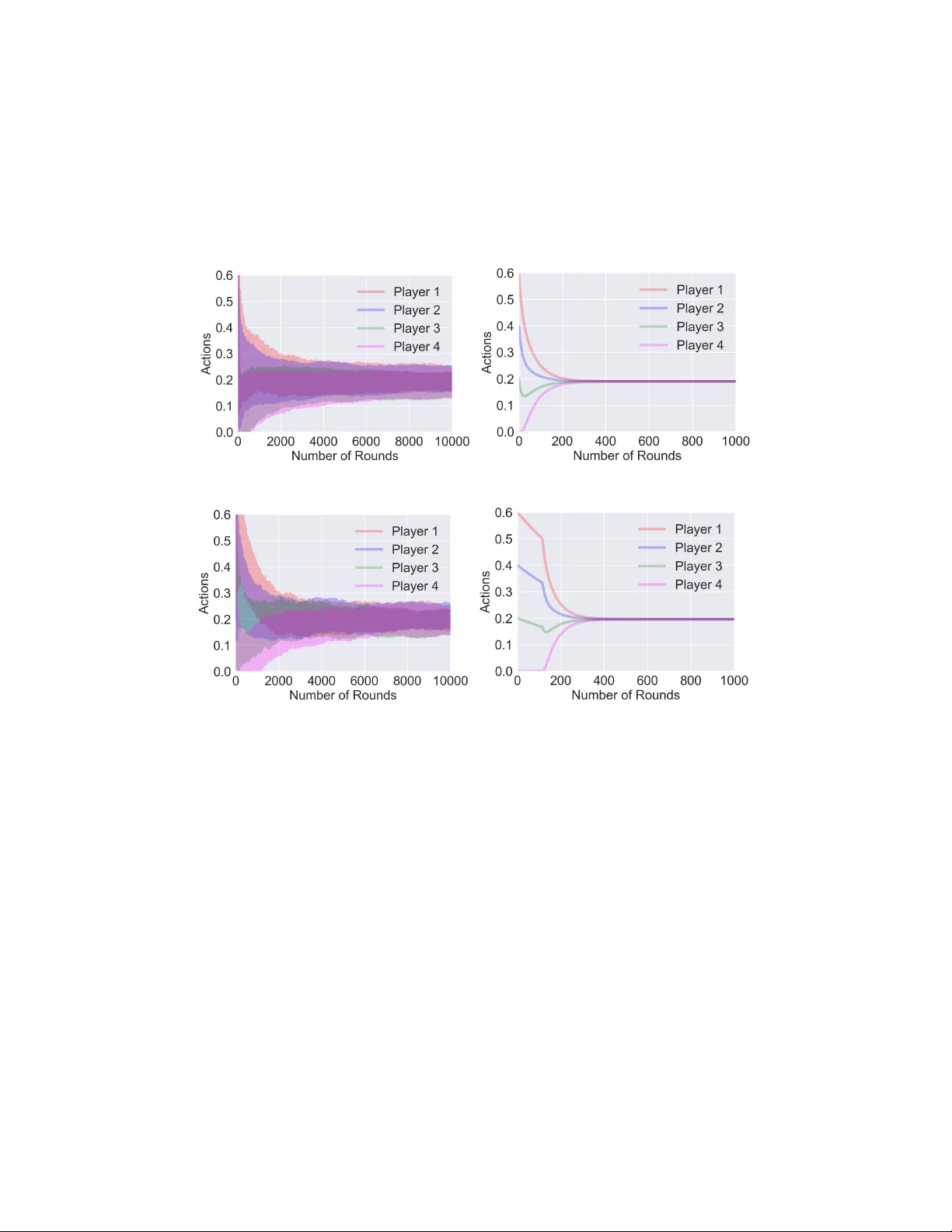
No-Regr et Lear ning in Cournot Games Y uanyuan Shi, Baosen Zhang Department of Electrical and Computer Engineering Univ ersity of W ashington yyshi, zhangbao@uw.edu Abstract This paper examines the con v ergence of no-re gret learning in Cournot games with continuous actions. Cournot games are the essential model for many socio- economic systems, where players compete by strategically setting their output quantity . W e assume that players do not ha ve full information of the game and thus cannot pre-compute a Nash equilibrium. T wo types of feedback are considered: one is bandit feedback and the other is gradient feedback. T o study the con ver gence of the induced sequence of play , we introduce the notion of con vergence in mea- sure, and show that the players’ actual sequence of action con ver ges to the unique Nash equilibrium. In addition, our results naturally extend the no-re gret learning algorithms’ time-av erage regret bounds to obtain the final-iteration con vergence rates. T ogether , our work presents significantly sharper conv ergence results for learning in games without strong assumptions on game property (e.g., monotonic- ity) and shows how exploiting the game information feedback can influence the con ver gence rates. 1 Introduction Game-theoretic models have been used to describe the cooperative and competiti ve behaviors of a group of players in various systems, including robotics, distributed control and socio-economic systems Li et al. (2019); Marden & Shamma (2015); Lanctot et al. (2017); Serrino et al. (2019). In this paper , we study the interaction of dynamic learning agents in Cournot games Cournot (1838). Cournot game is the essential market model for many critical infrastructure systems such as the energy systems Cai et al. (2019), transportation networks Bimpikis et al. (2014) and healthcare systems Chletsos & Saiti (2019). It is also one of the most pre valent models of firm competition in economics. In the Cournot game model, firms control their production lev el, which influences the market price Nada v & Piliouras (2010). For e xample, most of the US electricity mark et is b uilt upon the Cournot model Kirschen & Strbac (2004), where the generators bid to serve the demand in the power grid, and the electricity price is decided by the total amount of supply and demand. Each generator’ s payoff is calculated as the market price multiplying its share of the supply deducting any production cost. The goal of each player is to maximize its payoff by strate gically choosing the production quantity . Previous works in Cournot games mostly focus on analyzing the equilibrium behavior , especially the Nash equilibrium. Nash equilibrium describes a stable state of the system, as no player can gain anything by changing only their own strategy . Howe ver , it is not clear ho w players can reach the equilibrium if they do not start from one. Specifically , in the context of Cournot games, each player only has access to local information (i.e., his own payof f), and is not informed about the attributes of other participants. Thus, they cannot pre-compute, or agree on a Nash equilibrium before they be gin interacting. For these reasons, in this work, we mo ve a way from the static vie w of assuming players are at a Nash equilibrium. Instead, we analyze the long-run dynamics of learning agents in Cournot games, and ask the follo wing two fundamental questions: Preprint. W ork in progress. 1. W ill strate gic learning agents r each an equilibrium? 2. If so, how quic kly do they con verg e to the equilibrium? Reasoning about these questions requires specifying the dynamics, which describes ho w players adapt their actions before reaching the equilibrium. In particular , we consider the dynamics induced by no-regret learning algorithms. W e focus on no-regret learning algorithms for two main reasons. Firstly , it is a sensible choice for decision makers under limited information situations, as no one wants to realize that in hindsight the polic y they emplo yed is strictly inferior to a simple policy that takes the same action throughout. Secondly , it allows us to mak e minimal assumptions on the players’ decision policy . Different players can choose different algorithms, as long as the policy satisfies the no regret guarantee. In fact, no-re gret learning is an acti ve area of research and includes a wide collection of algorithms, and interested readers can refer to (Gordon, 2007; Hazan et al., 2016) for a detailed revie w . 1.1 Related W orks Dynamic beha vior in Cournot games has been studied before. Cournot Cournot (1838) considered the simple best response dynamics in his original paper , where players react to their opponents’ actions on the pre vious step. Cournot proved that the best response dynamics con verge to the unique Nash equilibrium (NE), after sufficiently many steps. Howe ver , his results only apply to two-player games. Since then, a rich set of literature has tried to generalize this result. For example, Milgrom & Roberts (1990) proposed an adapti ve behavior rule to reach the NE for an arbitrary number of players in Cournot games. Roughgarden (2016) sho wed that in Cournot games with linear price or cost function (hence a potential game), the best response dynamics con ver ge to the NE. Howe ver , all these best response dynamics require full information of other players’ pre vious actions and the exact game structure (i.e., price function, payof f functions). Howe ver , for man y applications of interest, pro viding full feedback is either impractical such as distributed control Marden & W ierman (2009) or explicitly disallowed due to pri vacy and mark et power concerns such as ener gy markets Ito & Reguant (2016). Studying the behavior of players under limited information is challenging, which starts to recei ve some recent attention. Most literature considers the no-regret dynamics because of their inherent robustness under uncertainty Bra vo et al. (2018). A general result about no-regret learning in games is that if all players experience no-regret as the time approaches infinity , the time-av erage action con verges to a coarse correlated equilibrium Roughgarden (2016); Syr gkanis et al. (2015); Foster et al. (2016). Ho we ver , coarse correlated equilibria (CCE) is a loose notion of equilibrium and may contain actions that are manifestly suboptimal for players Barman & Ligett (2015). In addition, besides the time-av erage behavior , players also care about their actual (or so called the final-iteration) behavior . Regarding the final-iteration con ver gence to a finer notion of equilibrium (e.g., Nash), assumptions on either game structure or player’ s action strategy , or both, are usually made. On the game structure side, Brav o et al. (2018) showed that the con vergence of online mirror descent (a no-re gret algorithm) with bandit feedback to the NE, in strongly monotone games 1 . Cohen et al. (2017) prov ed the con ver gence of multiplicati ve weights (also a no-regret algorithm) and Perkins et al. (2017) pro ved the con vergence of actor -critic reinforcement learning algorithm, both in potential games. Howe ver , a general Cournot game does not satisfy the monotone game and potential g ame definition, without further restrictions on the allo wed price function class (e.g., linear). On the action strategy side, Zhou et al. (2017, 2018); Mertikopoulos & Zhou (2019) relaxed the game structure assumption to variational stable games, which includes a broader range of games. But their proof only applies to online mirror descent (OMD) algorithm and does not generalize to all no-re gret dynamics. Similarly , Bervoets et al. (2016) assumed a specific action strategy and pro ved its con ver gence in games with concav e payof f functions. In summary , establishing general con ver gence in Cournot games under minimal game structure and behavioral hypotheses remains open. In the most relev ant result to our work, Nada v & Piliouras (2010) studied the no-regret dynamics in Cournot games with linear price functions and con ve x cost function. They proved the final- iteration con ver gence to the NE. Howe ver , as we will discuss in Section 2.3, Cournot games with their assumptions are monotone games thus the analysis are greatly simplified. Our work is a strict generalization of their results since we allow for a broad class of conca ve price functions. In fact, to 1 W e will formally define monotone games in Section 2.3. 2 the best of our kno wledge, our work is one of the fe w that obtain positi ve con vergence results without the monotonicity or stronger assumptions in the game structure. 1.2 Our Contributions In this work, we study the dynamics of no-regret learning algorithms in Cournot games, and our major contributions are in the follo wing three aspects. Firstly , we introduce a con ver gence notion which we call con ver gence in measur e . This con ver gence notion extends the standard conv ergence notion and permits negligible behavior variations (i.e., actions in a measure zero set). In fact, this notion allows us to treat the conv ergence question for general no-re gret algorithms, without ha ving to restrict ourselves to a specific subclass (such as online mirror descent Zhou et al. (2017); Mertikopoulos & Zhou (2019)). Secondly , we provide a detailed analysis of the long-run dynamics of no-regret learning in Cournot games. W e prove that both the time-av erage and final-iteration con verge to the unique Nash equilib- rium. The latter result on the limiting action of players has not be shown before. W e hav e no strong assumptions on the game structure (e.g., monotonicity) and no restrictions for the no-regret algorithm type. This is a much sharper result compared to the existing results on the time-av erage behavior con ver ging to a coarse correlated equilibrium Roughgarden (2016) or the final-iteration con vergence with specific game structure assumptions Brav o et al. (2018); Cohen et al. (2017). Thirdly , we deri ve the final-iteration con vergence rate under the notion of con vergence in measure, and link it to the time-average regret bounds of dif ferent no-regret algorithms. F or concreteness, we sho w that con vergence rate of zeroth-order FKM algorithm Flaxman et al. (2005) is O ( T − 1 / 4 ) and that of first-order OMD algorithm Shalev-Shwartz (2007) is O ( T − 1 / 2 ) . It provides quantitati ve insights for market designers on the benefit of releasing more information to the players, in terms of the market equilibration rate. 2 Problem Setup and Pr eliminaries In this section, we first introduce the Cournot game model and assumptions. Then, we provide two motiv ating examples of its applications in social infrastructure. Next, we revie w different types of no-regret learning algorithms and discuss the existing con vergence results and the difficulties of con ver gence analysis in Cournot games. 2.1 Model of Cournot Game Definition 1 (Cournot game Cournot (1838)) . Consider N players pr oduce homogenous pr oduct in a limited market, wher e the action space of each player is the pr oduction level ∀ i, x i ≥ 0 . The payoff function of player i is denoted as π i ( x 1 , ..., x N ) = p ( P N j =1 x j ) x i − C i ( x i ) , wher e p ( · ) is the mark et price function that maps the total pr oduction quantity to a price in R + , and C i ( · ) is the pr oduction cost function of player i . The goal of each player in Cournot games is to decide the best production quantity x i ≥ 0 such that maximizes his payoff π i . An important concept in game theory is the Nash equilibrium (NE), at which state no player can increase his payoff via a unilateral deviation in action. The analysis of NE is important since it re veals a stable state of the multi-agent system: once the NE is reached, no one would ha ve the economic incenti ve to break it. The NE of a Cournot game ( π 1 , ..., π N ) is defined by a vector x ∗ , such that ∀ i , π i ( x ∗ i , x ∗ − i ) ≥ π i ( x i , x ∗ − i ) , ∀ x i ≥ 0 , (1) where x − i denotes the actions of all players except i . The left side of Eq (1) is player i ’ s payoff at the NE, and the right side is that of any deviated action given other players’ actions fixed. In this paper , we restrict our attentions to Cournot games that satisfy the follo wing assumptions: Assumption 1. W e assume the Cournot games satisfy: 1) The market price function p is concave, strictly decr easing, and twice dif fer entiable on [0 , y max ] , where y max is the first point wher e p becomes 0 . F or y > y max , p ( y ) = 0 . In addition, p (0) > 0 . (A1) 3 2) The individual cost function C i ( x i ) is con vex, strictly incr easing, and twice dif fer entiable, with p (0) > C 0 i (0) , for all i . (A2) These assumptions are standard in literature (e.g., see Johari & Tsitsiklis (2005) and the references within). The assumption p (0) > C 0 i (0) is to avoid the tri viality of a player never participating in the game. Szidarovszk y & Y ako witz (1977) first prov ed that Cournot games with the above assumptions hav e unique Nash equilibrium. Proposition 1. A Cournot game satisfying (A1) and (A2) has exactly one Nash equilibrium. The proof of Proposition 1 is provided in Appendix B for readers’ reference. Belo w , we briefly discuss two example applications of Cournot g ame in socio-economic systems. Example 1 (Wholesale Electricity Mark et) The Cournot model is the most widely adopted framew ork for electricity market design Kirschen & Strbac (2004). Suppose there are N electricity producers, each supplying the market with x i units of energy . In an uncongested grid 2 , the electricity is priced as a decreasing function of the total generated electricity . For instance, consider both the market price and indi vidual production cost function are linear , the profit of generator i can be written as: π i ( x i ; x − i ) = x i ( a − b P N j =1 x j ) − c i x i , where c i ≥ 0 is the marginal production cost of i . Example 2 (Lotteries) Lotteries are becoming an increasingly important mechanism to allocate limited resources in social contexts, with examples in housing Friedman & W einberg (2014), park- ing Zhang et al. (2015) and buying limited goods Phade & Anantharam (2019). These lotteries typically allocate each player with a number of “coupons” and here we consider the coupon amount to be continuous (i.e., real numbers). The player’ s chance of winning depends on the number of coupons he owns, and the total number of coupons played in the round. Suppose x 1 , x 2 , . . . , x N are the coupons used by all players, then a decreasing price function p ( P i x i ) can be used to model the fact that each pla yer is less likely to win the lottery as others spend more coupons. The profit of player i is π i ( x i ; x − i ) = p ( P N j =1 x j ) x i − x i , where − x i represents the cost of spending the coupons. 2.2 Review of No-Regr et Algorithms The concept of Nash equilibrium is useful if players can reach it. Howe ver , in many practical settings, players do not have full information on the game (non-cooperati ve) and thus cannot pre-compute the NE beforehand. Thus the idea of “learning” the equilibrium arises and it becomes important to understand the dynamics of the iterati ve learning process. In this work, we focus on the class of learning algorithms with worst-case performance guarantees, namely the no-regret algorithms. An algorithm is called no-regret Hazan et al. (2016) (or no-external regret) if the dif ference between the total payoff it recei ves and that of the best-fixed decision in hindsight is sublinear as a function of time. Formally , at each time step t , an online algorithm A selects an action vector x t ∈ X . After x t is selected, the algorithm receiv es f t , and collects a payoff of f t ( x t ) . All decisions are made online, in the sense that the algorithm does not kno w f t before choosing action x t . Here all the payof f functions f 1 , f 2 , ..., f T ∈ F , where F is a bounded family of functions. Let T denote the total number of game iterations. Then the total payof f collected by algorithm A until T is P T t =1 f t ( x t ) , and the total payof f of a static feasible action ˜ x is P T t =1 f t ( ˜ x ) . W e formally define the regret of A after T iterations as: R T ( A ) = max x ∈X T X t =1 f t ( x ) − T X t =1 f t ( x t ) , (2) An algorithm A is said to hav e no re gret, if for e very online sequential problem, { f 1 , f 2 , ..., f T } ⊆ F , the regret is sublinear as a function of T , i.e., R T ( A ) = o ( T ) . This implies that the algorithm performs (at least) as well as the best-fixed strategy in hindsight. Such a guarantee is desirable for rational players since no one wants to realize that the decision policy he/she employed is strictly inferior to the same action throughout. There are a collection of algorithms satisfies the no-regret 2 In a congested grid, all electricity producers still compete in a Cournot game manner (i.e., bidding quantities), while the system operator that transmits electricity sets the congestion price to maximize social surplus of the entire system Y ao et al. (2008). 4 property , given the action set and the cost functions are both con ve x. Based on the information av ailable to players, no-regret algorithms can be grouped into two types: zeroth-order (or bandit) algorithms and first-order (or gradient-based) algorithms. Zeroth-order algorithms. It accounts for extremely lo w information en vironments where players hav e only the realized payof f information, i.e., f t ( x t ) obtained from a gi ven action x t and nothing else. In game-theoretic settings (especially in non-cooperati ve games), the bandit feedback frame work is more common since players usually only hav e local information and cannot tell with certainty what are the utilities and actions of other players. The core of zeroth-order no-regret learning algorithms is to infer the gradient, i.e., obtaining an unbiased gradient estimator with bounded variance. FKM Flaxman et al. (2005) is a well-kno wn zeroth-order no-regret algorithm under the single function e v aluation situation, which is also kno wn as “gradient descent without a gradient”. The pseudocode of FKM is provided in Appendix A1 (Algorithm 1). First-order algorithms. As opposed to the zeroth-order algorithms, in first-order algorithms, an oracle that returns the payof f gradient at the queried action (i.e., ∇ f t ( x t ) ) is assumed a vailable. Therefore, players can adjust their actions by taking a step to wards the gradient direction, to maximize their utilities. Online mirror descent Shalev-Shw artz (2007) is a widely adopted first-order no-regret algorithm, which has been extensi vely studied under the learning in games setting Zhou et al. (2017, 2018); Mertikopoulos & Zhou (2019). The pseudocode implementation of the online mirror descent algorithm is provided in Appendix A2 (Algorithm 2). W e want to emphasize that, the no-regret property only tells us about the time-a verage performance. From the players’ perspectiv e, they also care about (if not more) the performance of their final- iteration actions. Ho wev er , deri ving the final-iteration con ver gence based on the time-av erage regret is not easy . In this work, we prov e both the time-av erage and final-iteration con vergence of payof fs and actions, by ably using the Cournot game structure property , which we will discuss in more detail in Section 3. 2.3 Existing Con ver gence Results w .r .t. Cournot Game Existing learning in games literature mostly focus on the class of monotone games Rosen (1965). Definition 2 (Monotone game) . A game is monotone (or so called diagonally strictly concave) is it satisfies, ∀ x , x 0 ∈ X h g ( x ) − g ( x 0 ) , x − x 0 i ≤ 0 , (3) with equality if and only if x = x 0 , wher e g ( x ) is the game gradient that g ( x ) = [ ∇ 1 π 1 ( x ) , · · · , ∇ N π N ( x ) ] T . Rosen Rosen (1965) showed that every conca ve N-player game 3 satisfying this addittional mono- tonicity condition has a unique NE. He also showed that, starting from any feasible point in the action set, players will alw ays con ver ge to the NE, if the y adapt their actions follo wing the payof f gradients. In fact, Rosen’ s monotonicity condition is a common assumption and the cornerstone for many con vergence proofs in learning in g ames literature Brav o et al. (2018). Howe ver , general Cournot games with assumptions (A1) and (A2) may not satisfy the monotone condition. See the counter example below . Counter example Let consider a four-player Cournot game. The market price is a piecewise linear function with non-negati ve lo wer bound: p ( y ) =  1 − y 0 ≤ y ≤ 1 0 y > 1 and the individual production cost function is C i ( x i ) = 0 . 05 x i , ∀ x i ≥ 0 . Hence, the payoff of each player is: π i ( x ) = p ( 4 X j =1 x j ) x i − 0 . 05 x i , ∀ i = 1 , 2 , 3 , 4 . 3 A concave N-player game requires the action set to be conv ex and the indi vidual payoff function to be concav e in w .r .t. player’ s own action. Cournot games with assumptions (A1)-(A2) meet this definition. 5 The payoff gradient is ∂ π i ( x ) ∂ x i = 0 . 95 − P 4 j =1 x j − x i , when P 4 j =1 x j ≤ 1 , and ∂ π i ( x ) ∂ x i = − 0 . 05 otherwise. Consider the follo wing two points: x = [ 0 . 2082 , 0 . 2273 , 0 . 1988 , 0 . 2169 ] T and x 0 = [ 0 . 3506 , 0 . 3279 , 0 . 0456 , 0 . 4439 ] T . It is easy to check that, h g ( x ) − g ( x 0 ) , x − x 0 i = 0 . 0242 > 0 which contradicts the monotone g ame definition in Eq (3) . The above counter example sho ws that the pre viously examined models and con ver gence results in monotone games do not apply to Cournot games. In fact, without this nice game structure assumption, it becomes much harder to analyze the dynamics and deriv e con vergence results. 3 Con vergence Analysis in Cournot Games W e discuss the main con ver gence results in this section. The first step is to select the right notion of conv ergence. Next, we prov e the con ver gence results in two steps, by first sho wing the payoff con ver gence, then deri ving the action con ver gence. At the end of this section, we discuss the impact of different information and pricing mechanisms on the con ver gence rates. 3.1 Con ver gence Definition Definition 3 (Con ver gence in measure) . Let µ be a measure on N . W e say that a sequence a t con ver ges in measur e to a if ∀  > 0 , lim t →∞ µ ( | a t − a | >  ) = 0 . The reason we need to work with the notion of con ver gence in measur e rather than the standard notion of con ver gence (i.e., lim t →∞ a t = a ) is that the latter condition is too stringent for no-regret algorithms. Consider the following example. Gi ven a no-regret algorithm A , we can construct another algorithm A 0 in the follo wing manner . Let M be some positi ve inte ger larger than 1 . Then the actions produced by A 0 is the same as A except for times M , M 2 , M 3 , . . . . At these times, A ’ takes on the action 0 (or any other arbitrary action). Both A and A 0 are no-regret algorithms, since A 0 only de viates at a set of v anishing small fraction of points. On the other hand, for A 0 , its actions cannot conv er ge in the standard sense. Therefore, given only the regret bound, the best final time con ver gence result we can hope for is conv ergence in measure as defined in Definition 3. 3.2 Pay off Con vergence In this part, we pro ve the payof f con vergence. Theorem 1 sho ws the time-av erage con vergence and Theorem 2 sharps the result by showing the final-iteration con ver gence. Theorem 1 (T ime-av erage con vergence) . Suppose that after T iterations, e very player has expected r e gret o ( T ) . As T → ∞ , every player’ s time-average payoff 1 T P T t =1 π i ( x t ) , ∀ i , con verges to the payoff at the Nash equilibrium π i ( x ∗ ) . Pr oof. Consider the i -th player . In each game iteration t, let ( x t,i , x t, − i ) be the mov es played by all the players. From player i ’ s point of view , the payoff he obtains at time t is, ∀ ξ ∈ X i , π i ( ξ ) = π i ( ξ , x t, − i ) . (4) Note that this payoff function is conca ve with respectiv e to his o wn action ξ by assumption. By the definition of regret, R i ( T ) = max ˆ x i ∈X i T X t =1 π i ( ˆ x i , x t, − i ) − T X t =1 π i ( x t,i , x t, − i ) . (5) Equiv alently , ∀ ˆ x i ∈ X i , 1 T T X t =1 π i ( x t,i , x t, − i ) ≥ 1 T T X t =1 π i ( ˆ x i , x t, − i ) − R i ( T ) T . (6) 6 Let consider the best response of player i at time t giv en all other players’ actions as ( x ∗ t,i ) = arg max ξ π i ( ξ , x t, − i ) . Obviously , player i ’ s payoff is upper bounded by his best response payoff by definition, 1 T T X t =1 π i ( x t,i , x t, − i ) ≤ 1 T T X i =1 π i ( x ∗ t,i , x t, − i ) . (7) In addition, since π i is concav e with respect to x i , it follows: 1 T T X i =1 π i ( x ∗ t,i , x t, − i ) ≤ 1 T T X t =1 π 1 ( ˜ x i , x t, − i ) (8) where ˜ x i = P T t =1 x ∗ t,i T . Combining Eq. (6) and (8) we hav e, the difference between the actual payoff and best response is bounded by the regret, 1 T T X t =1 π i ( x t,i , x t, − i ) ≥ 1 T T X i =1 π i ( x ∗ t,i , x t, − i ) − R i ( T ) T . (9) Combine the lower bound in (9) and upper bound in (7), 1 T T X i =1 π i ( x ∗ t,i , x t, − i ) − R i ( T ) T ≤ 1 T T X t =1 π i ( x t,i , x t, − i ) , ≤ 1 T T X t =1 π i ( x ∗ t,i , x t, − i ) . (10) Since we know that R i ( T ) = o ( T ) as T → ∞ , use the Squeeze theorem in calculus, lim T →∞ 1 T T X t =1 π i ( x t,i , x t, − i ) = lim T →∞ 1 T T X t =1 π i ( x ∗ t,i , x t, − i ) , (11) which holds for all players. Therefore, as T → ∞ , the av erage payof f of each player con verges to the payoff at his best response. As every player plays his best response against the other players simultaneously , the time-av erage payof f con ver ges to the Nash equilibrium. Theorem 2 (Final-iteration con ver gence) . Suppose that after T iterations, every player has e xpected r e gret o ( T ) . As T → ∞ , every player’ s actual payoff π i ( x t ) , ∀ i , con ver ges to the payoff at the Nash equilibrium π i ( x ∗ ) in measur e, ∀  > 0 , lim t →∞ µ ( | π i ( x t ) − π i ( x ∗ ) | >  ) = 0 . Pr oof. W e prove Theorem 2 by contradition. In particular , suppose that ∃  > 0 , such that more than a sub-linear fraction of t ∈ { 1 , 2 , ..., T } satisfies that: | π i ( x t ) − π i ( x ∗ ) | >  . Let define the following notations for the proof. Denote a t = π i ( x ∗ t,i , x t, − i ) , which is the best response payoff for player i giv en others’ action, and b t = π i ( x t ) . Thus 0 ≤ b t ≤ a t , (12) No w , let re-arrange all the time steps such that the time where | b t − a t | >  show up in the front. Say there are T 1 such points, then lim T →∞ | 1 T T X t =1 ( b t − a t ) | = lim T →∞ 1 T T X t =1 | b t − a t | ( b t ≤ a t ) , = lim T →∞ ( 1 T T 1 X t =1 | b t − a t | + 1 T T X t = T 1 | b t − a t | ) ≥ lim T →∞ ( T 1 T  + 1 T T X t = T 1 | b t − a t | ) , (13) 7 Since T 1 accounts for more than a sub-linear fraction of T , we hav e T 1 T 9 0 as T → ∞ . Following Eq. (13), lim T →∞ | 1 T T X t =1 ( b t − a t ) | ≥ ( lim T →∞ T 1 T ) ·  > o ( T ) (14) which contradicts the definition of no-regret algorithms. Hence, giv en any  > 0 , as T → ∞ there exists at most a measure zer o set of time such that | b t − a t | >  . Since this holds for all players simultaneously , we have, ∀ i, lim T →∞ π i ( x t ) = π i ( x ∗ ) , ∀ t ∈ [1 , ..., T ] (15) for all but a measure zero set of time. One can interpret Theorem 2 from two angles. On the one hand, giv en any  > 0 (fix the error bound), the set of time that the actual payoff significantly deviates from the NE payoff equals R i ( T ) T . For no-regret algorithms with tighter regret bound, the set of time that far away from NE vanishes faster . On the other hand, after T time steps (fix the number of iterations), we hav e that ∀ i, | π i ( x t ) − π i ( x ∗ ) | < O ( R i ( T ) T ) , for all t ∈ T but a measure zero set. Thus, after the same number of iterations, algorithms with tighter regret bound ha ve smaller error bound. 3.3 Action Con ver gence Now we turn our attention to prove the action conv er gence. The follo wing two propositions are needed for the proof. Proposition 2 (In verse function theorem Stromberg (2015)) . Consider function f : R n → R n , and f ( x 0 ) = y 0 . Let J = ∂ f ∂ x | x = x 0 as the J acobian of function f . If J evaluated at x 0 is in vertible, then ther e e xists a continuous and differ entiable function g such that, g ( f ( x )) = x , for x ∈ X and y ∈ Y wher e X is some open set ar ound x 0 and Y is some open set ar ound y 0 . Proposition 3 (Lipschitz continuity) . A function f fr om X ⊂ R n into R n is Lipschitz continuous at x 1 ∈ X if ther e is constant L ∈ R + such that, || f ( x 2 ) − f ( x 1 ) || 2 ≤ L || x 2 − x 1 || 2 , for all x 2 ∈ X suf ficiently near x 1 . Theorem 3 (Con vergence in action) . Let x ∗ denote the Nash equilibrium, suppose that x satisfies: || π ( x ) − π ( x ∗ ) || 2 ≤  , (closeness in payoff) , then it implies that, || x − x ∗ || 2 ≤ L ·  , (closeness in action) , wher e π ( x ) = [ π 1 ( x ) , ..., π N ( x )] T is the payoff function/vector of a N-player Cournot game with assumptions (A1) and (A2), and L ∈ R + is a constant. Pr oof. Recall that the indi vidual payoff function in Cournot games is, π i ( x ) = p ( P N j =1 x j ) x i − C i ( x i ) , and π ( x ) = [ π 1 ( x ) , ..., π N ( x )] T is the collection of all players’ payoffs. Let J = ∂ π ∂ x denotes the Jacobian of function π ( x ) . Firstly , we show that J ( x ∗ ) is non-singular, where x ∗ is the NE. For the Jacobian entries, we ha ve J i,i ( x ∗ ) = ∂ π i ( x ) ∂ x i = 0 (diagonal entries) and J i,j ( i 6 = j ) ( x ∗ ) = ∂ π i ( x ) ∂ x j = p 0 ( P N j =1 x ∗ j ) x ∗ i (non-diagonal entries). Then the Jacobian equals, J ( x ∗ ) =     0 P ∗ x ∗ 1 · · · P ∗ x ∗ 1 P ∗ x ∗ 2 0 · · · P ∗ x ∗ 2 . . . P ∗ x ∗ N P ∗ x ∗ N · · · 0     . (16) 8 where P ∗ = p 0 ( P N j =1 x ∗ j ) is the market price at the NE. Concisely , J ( x ∗ ) can be written as, J ( x ∗ ) = P ∗ ( x ∗ · 1 T ) − P ∗ · diag ( x ∗ 1 , x ∗ 2 ..., x ∗ N ) . (17) W e argue that P ∗ > 0 (market price at the NE is positi ve). Suppose that at the NE, P i x ∗ i ≥ y max where y max is the first point such that p becomes zero. Th en at least one of the x ∗ i is positiv e, as by assumption p (0) > 0 . Ho we ver under this case, firm i can be strictly better off if it reduces x ∗ i , which contradicts the definition of NE. Therefore, we hav e P ∗ > 0 and P i x ∗ i < y max at the NE. Thus, in order to sho w J ( x ∗ ) is in vertible, it suf fices to sho w that  x ∗ · 1 T − diag ( x ∗ 1 , x ∗ 2 ..., x ∗ N )  is in vertible. Suppose v = [ v 1 , v 2 , ..., v N ] T solves the follo wing equation,  x ∗ · 1 T − diag ( x ∗ 1 , x ∗ 2 ..., x ∗ N )  v = 0 , (18) Since ∀ i, x ∗ i 6 = 0 (game admits no trivial solutions), the abov e linear system has the same solution as the following, ( 1 T v ) 1 − v = 0 . (19) which holds iff v = 0 . Therefore,  x ∗ · 1 T − diag ( x ∗ 1 , x ∗ 2 ..., x ∗ N )  is in vertible, and it follo ws J ( x ∗ ) is also in vertible. By the inv erse function theorem, as J ( x ∗ ) = ∂ π ∂ x | x = x ∗ is in vertible, there e xists a continuously differentiable function g (as the in verse function of π ) such that, g ( π ( x )) = x , ∀ π ∈ { ˆ π ∈ R n : || ˆ π − π ∗ || ≤  } , (20) By Lipschitz continuity , we hav e, || x − x ∗ || 2 = || g ( π ( x )) − g ( π ( x ∗ )) || 2 , ≤ L || π ( x ) − π ( x ∗ ) || 2 (21) Therefore, giv en the payof fs are close, i.e., || π ( x ) − π ( x ∗ ) || 2 ≤  , the actions will also be close, i.e., || x − x ∗ || 2 ≤ L ·  and L ∈ R + . 3.4 Con ver gence Rate The pre vious parts prov ed that the payof fs and actions both con verge to the NE of the game, under no-regret dynamics. Howe ver , the deriv ation steps do not explicitly provide us the con vergence rate. In this part, we complete the analysis by discussing the conv ergence rate. Recall that the payoff con ver gence is based on the following equation (Eq (10) in Section 3.2), 1 T T X i =1 π i ( x ∗ t,i , x t, − i ) − R i ( T ) T ≤ 1 T T X t =1 π i ( x t,i , x t, − i ) ≤ 1 T T X t =1 π i ( x ∗ t,i , x t, − i ) , where R i ( T ) is the algorithm regret after T iterations. Therefore, the rate of con ver gence naturally connects to the algorithm’ s regret bound. Zeroth-order algorithm Flaxman et al. (2005) provides that the re gret bound of FKM algorithm is R ( T ) = O ( T 3 4 ) . By Theorem 2, we have that, || π ( x t ) − π ( x ∗ ) || 2 ≤ O ( R ( T ) T ) = O ( T − 1 4 ) , for all t (except a measure zero set of time steps), as T goes to infinity . Since the payof f is bounded, by Theorem 3, the action is also bounded || x t − x ∗ || 2 ≤ O ( T − 1 4 ) for all b ut a measure zero set of time. 9 First-order algorithm The regret bound for online mirror descent (OMD) is R ( T ) = O ( T 1 2 ) Hazan et al. (2016). Similarly , we ha ve that, || π ( x t ) − π ( x ∗ ) || 2 ≤ O ( R ( T ) T ) = O ( T − 1 2 ) , for all t but a measure zero set, as T goes to infinity . By Theorem 3, the action is also bounded by || x t − x ∗ || 2 ≤ O ( T − 1 2 ) for all but a set of measure zero time. Comparing the con ver gence rates between zeroth-order algorithms and first-order algorithms, we find that the benefits of ha ving access to the gradient information are O ( T − 1 4 ) in terms of player’ s equilibration rate. Using this insight, it is interesting to think from the market operator’ s shoe. In most current markets (e.g., electricity mark et), the system operator only provides the zeroth-order information for participants. Howe ver , our results suggest that by offering more information, the market (aggreg ate production lev els, prices) can con ver ge to the stable state faster . This observ ation provides a ne w angle to the vast amount of economics literature (e.g., Athey & Le vin (2018) and the references within) on studying the value of information in game ef ficiency . Our results imply that sharing more information can not only impro ve mark et ef ficiency b ut will also contrib ute to better computational performance. 3.5 Discussion on Game Structure and Con vergence Finally , we discuss how the con ver gence rate is affected by the game structure. In section 2.3, we gav e a counter e xample sho wing that Cournot games may not be monotone games. But what if we restrict the price and individual cost function class such that Cournot games satisfy the monotonicity property? Will it lead to dif ferent con vergence rates? For e xample, consider a Cournot game with linear price function P ( P N i =1 x i ) = 1 − P N i =1 x i and linear individual cost C i ( x i ) = x i , ∀ i . By simple calculation, we find that this game is not only monotone but also strongly monotone in a sense that, X i ∈ N λ i h g i ( x 0 ) − g i ( x ) , x 0 − x i ≤ − β 2 || x 0 − x || 2 , (22) for some λ i , β > 0 and for all x , x 0 ∈ X . Bra v o et al. (2018) pro ved that in strongly monotone games, zeroth-order no-regret algorithms can achie ve O ( T − 1 3 ) con ver gence rate, and first-order algorithms hav e O ( T − 1 ) con ver gence rate. Compared to our results in general Cournot games, that is O ( T − 1 4 ) for zeroth-order algorithms and O ( T − 1 2 ) for first-order algorithms, the benefits of using linear price function and having the strongly monotone property can be measured quantitatively . This provides yet another useful insight for market designers on the impact of price function design (hence the game property) on the market equilibration rate, in addition to the information mechanism design. 4 Numerical Experiments W e provide two Cournot game examples and visualize the no-re gret dynamics in these games. These toy e xamples aim to help readers quickly grasp the ke y theoretic results from three perspecti ves: 1) the con vergence beha vior; 2) the con vergence rate dif ferences between zeroth-order and first-order no-regret algorithms; and 3) the impact of game structure on con ver gence rates. Setup W e consider two four -player Cournot games with dif ferent market price and indi vidual cost functions. G1: a monotone Cournot game where p ( x ) = 1 − ( P i x i ) , and a linear production cost function is C i ( x i ) = 0 . 05 x i . G2: a Cournot game that is not monotone. W e take the counter e xample in Section 2.3 that the price function is piece wise linear that p ( x ) = 1 − ( P i x i ) , 0 ≤ P i x i ≤ 1 and p ( x ) = 0 otherwise. The individual production cost is C i ( x i ) = 0 . 05 x i , ∀ x i ≥ 0 . The Nash equilibrium for both games is x ∗ 1 = x ∗ 2 = x ∗ 3 = x ∗ 4 = 0 . 19 , lev eraging the fact we proved within Theorem 3 that P i x ∗ i ≤ y max for G2. Both games proceed as follo ws. At each time step, e very player simultaneously picks a production lev el, and then the mark et price is determined by their joint production and broadcasted back to all 10 players. Each player calculates his own payof f by multiplying the production lev el by the market price, subtracting the cost. According to the observed payoff, players adjust their action strategies for the next round. The game is repeated for multiple times with players either all using the zeroth-order FKM algorithm or the first-order OMD algorithm. The algorithm implementation details can be found in Appendix A3. In the OMD case, each player’ s payoff gradient is also calculated and broadcasted back to the corresponding player . W e record the actions, payof fs, and the market price at each round. (a) G1: FKM (b) G1: OMD (c) G2: FKM (d) G2: OMD Figure 1: Conv ergence beha vior of FKM and OMD in two e xample Cournot games. Fig. 1 shows that all players’ actions con ver ge to the NE under both games, for both FKM and OMD algorithms. Ho we ver , the conv ergence rate dif fers significantly . Comparing the performance of FKM (left column) against the performance of OMD (right column), it is obvious that the conv ergence rate of OMD is much faster , which demonstrates the benefits of having access to the payoff gradient information. In addition, viewing the con vergence rate dif ference between G 1 (upper ro w) and G 2 (bottom row), we find that the conv ergence is faster in G 1 when the game is monotone, for both algorithms. This illustrates the gain of certain game structure. These observations are aligned with the theoretical results in Section 3. 5 Conclusion In this paper, we study the interaction of strategic players in Cournot games with concave price functions and con ve x cost functions. W e consider the dynamics of players actions and payoffs when all players use no-re gret algorithms. W e prove the time-a verage and final-iteration con ver gence for both payof fs and actions. Furthermore, we quantify the value of information and g ame structure in terms of players’ con vergence rates. It suggests that different information and game structures can lead to faster con vergence rate, which provides insights for mark et mechanism design with Cournot models. Our work is a strict generalization of all pre viously e xamined models, as they apply to all no-regret dynamics in general Cournot games, without game structure assumptions and restrictions on the type of algorithms. 11 References Athey , S. and Levin, J. The value of information in monotone decision problems. Researc h in Economics , 72(1):101–116, 2018. Barman, S. and Ligett, K. Finding any nontrivial coarse correlated equilibrium is hard. A CM SIGecom Exchanges , 14(1):76–79, 2015. Bervoets, S., Bra v o, M., and Faure, M. Learning and con vergence to nash in games with continuous action sets. T echnical report, W orking paper , 2016. Bimpikis, K., Ehsani, S., and Ilkiliç, R. Cournot competition in networked mark ets. In Pr oceedings of the 15th A CM Confer ence on Economics and Computation (EC 2014) , pp. 733, 2014. Brav o, M., Leslie, D., and Mertikopoulos, P . Bandit learning in concave n-person games. In Pr oceedings of the 32nd International Confer ence on Neural Information Pr ocessing Systems (NeurIPS 2018) , pp. 5661–5671, 2018. Cai, D., Bose, S., and Wierman, A. On the role of a market maker in networked cournot competition. Mathematics of Operations Resear ch , 44(3):1122–1144, 2019. Chletsos, M. and Saiti, A. Hospitals as suppliers of healthcare services. In Str ate gic Manag ement and Economics in Health Car e , pp. 179–205. Springer , 2019. Cohen, J., Héliou, A., and Mertikopoulos, P . Learning with bandit feedback in potential games. In Pr oceedings of the 31st International Confer ence on Neural Information Pr ocessing Systems (NeurIPS 2017) , pp. 6372–81, 2017. Cournot, A.-A. Recher ches sur les principes mathématiques de la théorie des richesses par Augustin Cournot . chez L. Hachette, 1838. Flaxman, A. D., Kalai, A. T ., Kalai, A. T ., and McMahan, H. B. Online con vex optimization in the bandit setting: gradient descent without a gradient. In Pr oceedings of the 16th annual A CM-SIAM symposium on Discr ete algorithms (SOD A 2005) , pp. 385–394, 2005. Foster , D. J., Li, Z., L ykouris, T ., Sridharan, K., and T ardos, E. Learning in games: Rob ustness of fast con vergence. In Pr oceedings of the 30th International Confer ence on Neural Information Pr ocessing Systems (NeurIPS 2016) , pp. 4734–4742, 2016. Friedman, J. H. and W einberg, D. H. The economics of housing voucher s . Academic Press, 2014. Gordon, G. J. No-regret algorithms for online conv ex programs. In Pr oceedings of the 21st International Confer ence on Neur al Information Pr ocessing Systems (NeurIPS 2007) , pp. 489–496, 2007. Hazan, E. et al. Intr oduction to online conve x optimization . Foundations and T rends in Optimization., 2016. Ito, K. and Reguant, M. Sequential markets, market po wer , and arbitrage. American Economic Revie w , 106(7):1921–57, 2016. Johari, R. and Tsitsiklis, J. N. Efficienc y loss in cournot games. Harvar d University , 2005. Kirschen, D. S. and Strbac, G. Fundamentals of power system economics , volume 1. Wile y Online Library , 2004. Lanctot, M., Zambaldi, V ., Gruslys, A., Lazaridou, A., T uyls, K., Pérolat, J., Silver , D., and Graepel, T . A unified game-theoretic approach to multiagent reinforcement learning. In Pr oceedings of the 31st International Confer ence on Neural FInformation Pr ocessing Systems (NeurIPS 2017) , pp. 4193–4206, 2017. Li, Y ., Carboni, G., Gonzalez, F ., Campolo, D., and Burdet, E. Dif ferential game theory for versatile physical human–robot interaction. Natur e Machine Intellig ence , 1(1):36–43, 2019. Marden, J. R. and Shamma, J. S. Game theory and distributed control. In Handbook of game theory with economic applications , pp. 861–899. Elsevier , 2015. 12 Marden, J. R. and Wierman, A. Overcoming limitations of game-theoretic distrib uted control. In Pr oceedings of the 48h IEEE Conference on Decision and Contr ol (CDC 2009) , pp. 6466–6471, 2009. Mertikopoulos, P . and Zhou, Z. Learning in games with continuous action sets and unkno wn payoff functions. Mathematical Pr ogramming , 173(1-2):465–507, 2019. Milgrom, P . and Roberts, J. Rationalizability , learning, and equilibrium in games with strategic complementarities. Econometrica , 58(6):1255–77, 1990. Nadav , U. and Piliouras, G. No regret learning in oligopolies: cournot vs. bertrand. In Proceedings of the 11th A CM Confer ence on Economics and Computation (EC 2010) , pp. 300–311, 2010. Perkins, S., Mertikopoulos, P ., and Leslie, D. Mixed-strategy learning with continuous action sets. IEEE T ransactions on Automatic Contr ol , 62(1):379–384, 2017. Phade, S. and Anantharam, V . Optimal resource allocation over networks via lottery-based mecha- nisms. In International Confer ence on Game Theory for Networks (Gamenets 2019) , pp. 51–70. Springer , 2019. Rosen, J. B. Existence and uniqueness of equilibrium points for concave n-person games. Economet- rica , pp. 520–534, 1965. Roughgarden, T . T wenty lectur es on algorithmic game theory . Cambridge Univ ersity Press, 2016. Serrino, J., Kleiman-W einer , M., Parkes, D. C., and T enenbaum, J. Finding friend and foe in multi-agent games. In Pr oceedings of the 33r d International Confer ence on Neural Information Pr ocessing Systems (NeurIPS 2019) , pp. 1249–1259, 2019. Shalev-Shw artz, S. Online learning: Theory , algorithms, and applications . PhD thesis, Hebre w Univ ersity of Jerusalem, 2007. Stromberg, K. R. An intr oduction to classical r eal analysis , volume 376. American Mathematical Society , 2015. Syrgkanis, V ., Agarw al, A., Luo, H., and Schapire, R. E. Fast con vergence of re gularized learning in games. In Pr oceedings of the 28th International Confer ence on Neur al Information Pr ocessing Systems (NeurIPS 2015) , pp. 2989–2997, 2015. Szidarovszk y , F . and Y ako witz, S. A new proof of the existence and uniqueness of the cournot equilibrium. International Economic Revie w , pp. 787–789, 1977. Y ao, J., Adler , I., and Oren, S. S. Modeling and computing two-settlement oligopolistic equilibrium in a congested electricity network. Operations Resear ch , 56(1):34–47, 2008. Zhang, B., Johari, R., and Rajagopal, R. Competition and coalition formation of rene wable po wer producers. IEEE T ransactions on P ower Systems , 30(3):1624–1632, 2015. Zhou, Z., Mertikopoulos, P ., Moustakas, A. L., Bambos, N., and Glynn, P . Mirror descent learning in continuous games. In 2017 IEEE 56th Annual Confer ence on Decision and Contr ol (CDC 2017) , pp. 5776–5783, 2017. Zhou, Z., Mertikopoulos, P ., Athey , S., Bambos, N., Glynn, P ., and Y e, Y . Learning in games with lossy feedback. In Pr oceedings of the 32nd International Confer ence on Neural Information Pr ocessing Systems (NeurIPS 2018) , pp. 5140–5150, 2018. 13 A ppendix A A1. Review of FKM FKM Flaxman et al. (2005) is a well-known zeroth-order no-re gret algorithm under the single function ev aluation situation, which is also known as “gradient descent without a gradient”. The pseduocode of FKM is giv en in Algorithm 1 (reproduced from Hazan et al. (2016)). Algorithm 1 FKM Hazan et al. (2016) Input: decision set X , parameters δ , η . Pick y 1 = 0 (or arbitrarily). for t = 1 , 2 , ..., T do Draw u t ∈ S d uniformly at random, and set x t = y t + δ u t . Play x t suffer loss f t ( x t ) . Calculate g t = n δ f t ( x t ) u t . Update y t +1 = Q X δ [ y t − η g t ] . end for A2. Review of Online Mirror Descent Online mirror descent (OMD) Shalev-Shwartz (2007) is a widely adopted first-order no-regret algorithm, which has been extensi vely studied under the learning in games setting Zhou et al. (2017, 2018); Mertikopoulos & Zhou (2019). The pseudocode of OMD is provided in Algorithm 2 (reproduced from Hazan et al. (2016)). Algorithm 2 Online Mirror Descent with Quadratic Regularization Hazan et al. (2016) Input: decision set X , parameter η > 0 , regularization function R ( x ) = 1 2 || x || 2 2 which are strongly con ve x and smooth. Pick y 1 = 0 (or arbitrarily) and x 1 = arg min x ∈X || y 1 − x || 2 2 . for t = 1 , 2 , ..., T do Play x t . Observe the payof f function gradient ∇ f t ( x t ) . Update y t according to the rule: [Lazy version] y t +1 = y t − η ∇ f t ( x t ) [Agile version] y t +1 = x t − η ∇ f t ( x t ) Project to feasible set: x t +1 = arg min x ∈X || y t +1 − x || 2 2 end for A3. Implementation Details For the FKM implementation, we ha ve X = R + as the feasible action set. W e set η t = η 0 (0 . 1 t ) 3 / 4 , δ = δ 0 t 1 / 3 , and η 0 = 0 . 05 , δ 0 = 1 for all experiments. For the OMD implementation, we use the agile version update and quadratic regularization. Similarly , the action feasible set is X = R + . W e set η = 1 2 √ T as suggested in Hazan et al. (2016) Theorem 5.6 and T = 1000 . All experiments were run on a MacBook Pro with 16 GB 2400 MHz DDR4 memory , and a 2.2GHz Intel Core i7 CPU. 14 A ppendix B Proof of Pr oposition 1 Proposition (Restatement of Proposition and Assumptions) . A Cournot game satisfying the following assumptions: 1) The market price function p is concave, strictly decr easing, and twice dif fer entiable on [0 , y max ] , where y max is the first point wher e p becomes 0 . F or y > y max , p ( y ) = 0 . In addition, p (0) > 0 . (A1) 2) The individual cost function C i ( x i ) is con vex, strictly incr easing, and twice dif fer entiable, with p (0) > C 0 i (0) , for all i . (A2) has exactly one Nash equilibrium. Pr oof. Define the total production s = P n i =1 x i . For each player i , and each s ≥ 0 , define x i ( s ) =  x, such that x ≥ 0 and p ( s ) = C 0 i ( x ) − xp 0 ( s ) . 0 , if no such exists . Note that x i ( s ) is monotone decreasing in s and x i ( s ) is continuous in s . It is no w sho wn that there is a unique non-negati ve number s ∗ such that, X x i ( s ∗ ) = s ∗ . (23) For P x i (0) ≥ 0 and by the positi vity of C 0 i , − p 0 , P x i ( ξ ) = 0 < ξ for any ξ such that f ( ξ ) = 0 . As x ( s ) = P N i =1 x i ( s ) is continuous and strictly decreasing for any s such that x ( s ) > 0 , there must be exactly one s ∗ for which x ( s ∗ ) = s ∗ . By the definition of x i ( s ) , each x i ( s ) maximizes π i ( x 1 , ..., x N ) = p ( P N j =1 x j ) x i − C i ( x i ) ; therefore, x ( s ∗ ) = ( x 1 ( s ∗ ) , ..., x N ( s ∗ )) is an equilibrium point of the model, and no other point can be an equilibrium point. The abov e proof is reproduced from Szidarovszky & Y akowitz (1977) for reader’ s easy reference. 15