Correction of Chromatic Aberration from a Single Image Using Keypoints

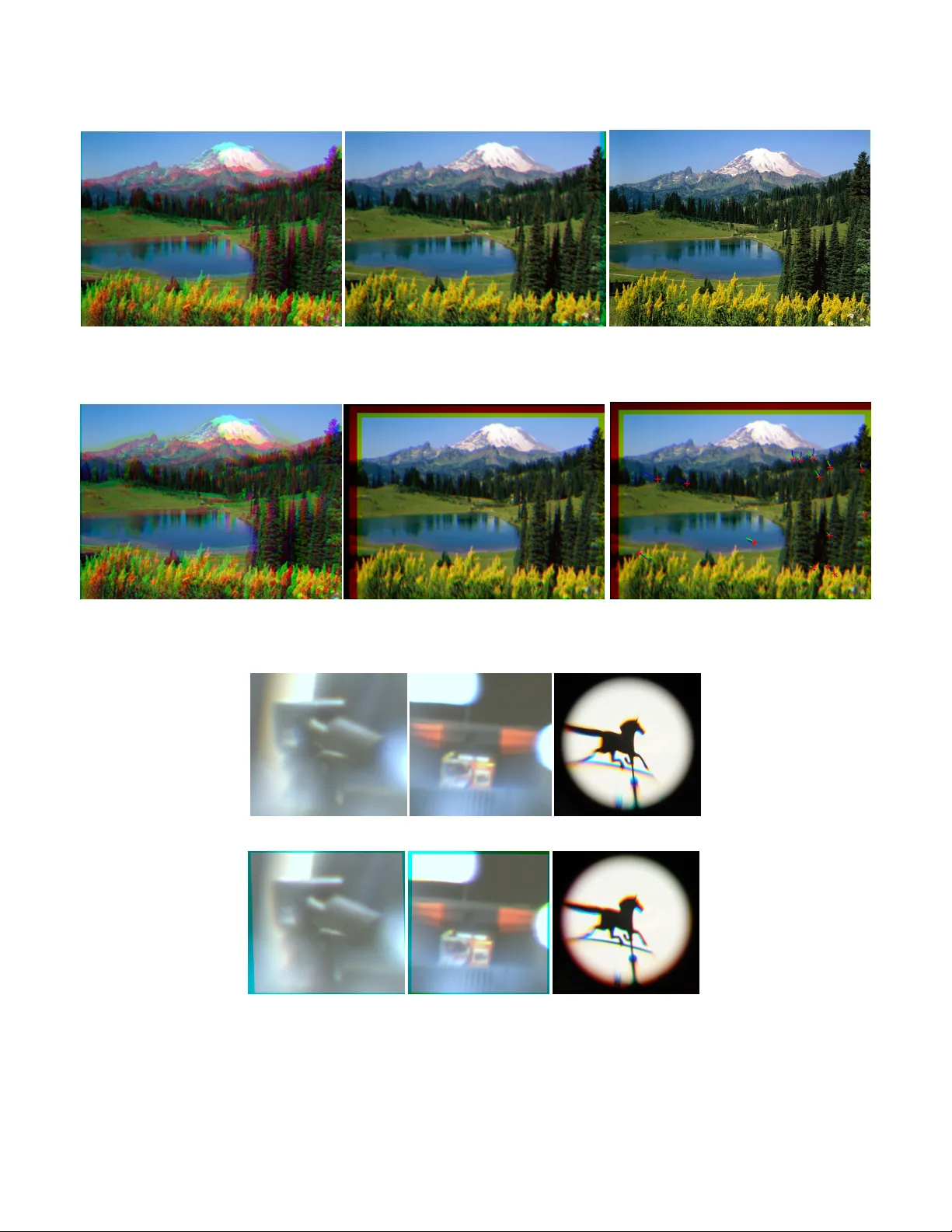
Correction of Chromatic Aberration from a Single Image Using K eypoints BENJAMIN T . CECCHET TO, Department of Computer Science, The University of British Columbia In this paper , we propose a method to correct for chromatic aberration in a single photograph. Our method replicates what a user would do in a photo editing program to account for this defect. W e nd matching keypoints in each colour channel then align them as a user would. CCS Concepts: • Computing methodologies → Computational photography ; Image pr ocessing . Additional Key W ords and Phrases: chromatic aberration, image pro- cessing, color , 1 IN TRODUCTION Chromatic aberration (also known as colour fringing) is a phenom- ena where dierent wav elengths of light refract through dierent parts of a lens system. Thus, the colour channels may not align as they reach the sensor/lm. This is most notable in cheaper lenses, it is also noticeable at higher resolutions. W e desire an image fr ee of chromatic aberrations is simple, so all the planes are in focus. For a simple lens system this amounts to misaligned colour channels (r ed, green and blue). The misalignment is due to a uniform scaling and translation. There are many types of other chromatic aberrations. Complex lens assemblies introduce new distortions. W e propose a method to deal with the simple, more common scenario. W e later discuss possible ways to deal with more complex ones. 2 PREVIOUS W ORK Many domains have sought to correct chromatic aberration. A major goal is to improv e accuracy of measurement. This could be either in a lab or more constrained capture scenarios such as of space. One such method is in active optics [Willson and Shafer 1991]. For active optics, instead of taking one e xposure for the colour channels simultaneously , the user takes one for each exposure at dierent times. Each time, the focus changes to match the channel’s optimal plane. This accounts for the aberration in the lens so the three channels will align in the nal result. This requires a change fr om traditional hardware as w ell as three exposures at thr ee points in time. This limits capture for dynamic scenes, as the object may be moving in that time span. Another proposed metho d is to model the edge displacements with cubic splines to compute a nonlinear warp of the image [Boult and W olberg 1992]. This method cannot handle blurring/defo cus in the image plane along with saturation eects. It breaks down in re- gions that are either underexposed or overexposed. A dierent tech- nique exists for correcting lateral chromatic aberration where one calculates the aberrations and uses warping to compensate [Mallon and Whelan 2007]. This only works for calibrated cameras/images which may not be workable for a more simple user . Chromatic aberrations can also determine depth information without prior calibration [Garcia et al. 2000]. Recently , an analysis of aberrations show they are not a simple shift of colour planes. W e can get a corrected result by computing a non-linear warp [K ang 2007]. This algorithm handles many dierent categorized cases of aberrations. Its only limitations are artifacts caused by saturation, and slow , non-linear , performance. Since we want to deal with the simple case, we may want to remove perspective distortions. A few algorithms hav e solved this problem in the past [Swaninathan et al . 2003]. If we undistort a lens distortion, we should end up with only needing to solve for the translation/scaling of the colour channels to align them. A recently proposed metric, L , can determine a depth matte from a colour-ltered aperture [Bando et al . 2008]. This metric measures how collinear and correlated points are in 3D (colour space). It is then used to nd a disparity from their custom colour-ltered aperture. 3 O VERVIEW Instead of concentrating on the optical derivation, we instead con- sider an image-based one. An artist can align colour channels of an image to correct the aberration. They align the channels by moving the corners of the images to transform each channel’s image. W e attempt to automate this artist driven result. The main idea is to align two of the colour channels to the third one. The green channel has the least amount of aberration as it is in the middle of the colour spectrum. In some of the results, we match to the red channel for simplicity . Choosing a dierent channel to match to results in a scaled version of the corrected image. Our solution is to nd keypoints in all channels, and nd where the keypoints match to the xed channel. At the same time, we minimize the aberration metric L . This is like nding disparities in stereo, but in 3 channels instead of two images. Once we have these matchings, we can prune the r esults based on how well the matchings are. Then we ne ed to nd a transformation from the non-xed colour planes to the xe d one. W e restrict the transfor- mation to a scale and translation. W e solv e the issues that arise from saturation by ignoring saturated regions and their neighbours. Since the algorithm is linear , it is quite ecient. 3.1 Computing the Alignment Metric Before we start describing how to nd the keypoints, and disparities, it is best to dene how aligned the colour channels are. It is not suitable to do cross-correlation, as that only tells us how aligned two colour channels are. W e want to see how aligned three are. As described above, there exists such a metric L [Bando et al . 2008]. For a given neighb ourhood around a pixel ( x , y ) , with eigenvalues of the covariance matrix trix λ i and covariance matrix diagonal elements σ 2 r , σ 2 д , σ 2 b , L ( x , y ) = λ 0 λ 1 λ 2 σ 2 r σ 2 д σ 2 b 1 Benjamin T . Ceccheo (a) (b) Fig. 1. (a) A photo with chromatic aberration. (b) A correction for it using our algorithm. [Foundation 2009] (a) (b) Fig. 2. L values over the images in Figure 1. This value is essentially how collinear the colour points in this neighbourhood are in RGB-space. These are visualized in Figure 3. The lower this value is, the more collinear the p oints are and the higher the less collinear . As mentioned in the appendix of the paper , this can be considered to be related to cross-correlation, and is thus exactly what we want to use. How to choose this neighbourhoo d size is a dierent story . The smaller it is, the less statistics we have about that neighbourhood and thus may have a worse matching. The larger it is, the better chance w e have of a matching, however the longer it takes. This value is bounded between 0 and 1, as mentioned in the paper . If w e show this for ev ery pixel as in Figure 2, we can see that images without chromatic aberration show very little misalignment over the whole image. Another justication of using this metric is that according to the colour lines model [Omer and W erman 2004], colour points in RGB-space of the whole image will lie along dierent colour lines. If we look at smaller neighb ourhoods, then we can assume the points will also lie along either a line, or intersection of lines. This measures the collinearity of those neighbourho ods. If we search for an ideal alignment, then we want to maximize the collinearity , thus minimizing L . 3.2 Finding Ke ypoints The rst task is to nd regions wher e the keypoints would be useful. W e want to nd regions where the alignment measur e L is very high, but at the same time we want to b e certain there is a goo d possibility for a good alignment. Choosing regions in the image with high L values is costly , as we have to compute L for every pixel and examine that image . Also , it is not guaranteed to give us a good pixel, such as smooth regions which may have ambiguous results. A good choice would be to nd high gradient r egions and use points from those. Specically where we know there is an edge nearby . This gives us a better match since we know the other two channels should have a high gradient in that region too. W e randomly sample from the norm of the gradient image with gradient suciently high within a threshold. In addition, if we want to pay the cost of the L image, we can compute it only in regions where the norm of the gradient is suciently high. If we multiply L by the norm of the gradient image, and threshold it, we can sample points that are highly unaligne d with enough information around them to be aligned. 3.3 Finding Disparities If we want to align two channels to the remaining one (say align green and blue to the red channel), we need to shift over all combi- nations of possible windows, with dierent scales. The idea is w e want the neighbourhood of the gr een and blue channels to be corre- lated with the red, and those channels we know may be elsewhere with a dierent scale. Thus, we want to minimize the misalignment L ( x , y ) subject to a shifted and scaled window in both green and blue channels so we can write L ( x , y ; d G x , d G y , σ G , d B x , d B y , σ B ) 2 Correction of Chromatic Aberration from a Single Image Using Keypoints Fig. 3. Colour points ( r , д , b ) in neighbourhood clusters ar ound a pixel. Le: From a control image with no aberrations chosen randomly . Right: From a photo with aberrations, chosen at regions of obvious colour fringing. (a) (b) Fig. 4. Zoomed in area from Figure 1. (a) Original photo . (b) Corrected. With disparities d x , d y and relative scales σ . Where we iterate over all acceptable disparities (as in stereo) and all acceptable scales. W e know howe ver , that the disparities and cale dierence should- nâĂŹt be too large (unless one has a truely horrible lens) so we can limit the search to local neighbourhoods in that sixtuple. In fact, if the scale dierence is decently small (which it usually is in the case of aberrations) we can simply look for disparities to nd the scale aspect of the transform. Thus we can write L as L ( x , y ; d G x , d G y , d B x , d B y ) T o be able to handle dierent scales, one could simply do an image pyramid based approach as in other computer vision papers. This is unnecessary , as most aberrations are not that distant in the scale domain. The reason why this works is if we have a perfect edge (all one colour on one side, then all the other colour on the other side of the edge) in an image then the colours in the neighbourhood will cluster into two distinct regions. Since we are dealing with a natural image and edges are not p erfect, these clusters will connect in a line as there will be a gradient from one colour to the other . If the image is misaligned, then this region will become more spread out. Now if we consider a multicolour ed region, we get a more complicated shape. Howev er , if we nd disparities that minimizes this clusterâĂŹs collinearity , we should get a better aligned image since weâĂŹre minimizing the spread of the whole shape. 3.4 Pruning Ke ypoints Although weâĂŹve found ke ypoints and disparities for those key- points in the other two channels, they might not give us go od information. For example, if the best matching L value for the point neighbourhood was high, w e shouldnâĂŹt want to use that point as it is not a very well aligned point. W e only want to use p oints that have gone from high L value (unaligned) to low L value (aligned). Since we only chose points that are unaligne d, we just need to prune away the points that r emain unaligned. Thus we only choose points with a low enough ne w L value. Alternatively , since we know we want to do a scale and translation for each channel (3 degrees of freedom for each) we only need 2 ke ypoints (each being 2 dimen- sional). Thus we could choose the 2 keypoints with the lowest L value. Other methods could include weighting the keypoints based on the L parameter and havenâĂŹt been fully explored. In practice, thresholding by the right amount is sucient for good results. 3.5 Computing Image Transforms Now that we have a set of good points, we can solve for the transfor- mation pretty easily . Let us consider the red and green channels for now . W e have ( p R x , p R y ) chosen in the xed red channel and a p oint translated by disparity in the green channel ( p G x , p G y ) . W e have the equation: ©  « σ G 0 t G x 0 σ G t G y 0 0 1 ª ® ¬ ©  « p R x p R y 1 ª ® ¬ = ©  « p G x p G y 1 ª ® ¬ Thus we can rearrange it for this point pair as:  p R x 0 1 p R y 1 0  ©  « σ G t G x t G y ª ® ¬ =  p G x p G y  If we have a second point we can solv e this system for σ G , t G x , t G y , the scale, and translation respectively . In practice, weâĂŹd want more than just two p oints because the p oints might have only a good local solution and not global. Thus weâĂŹd want points from dierent regions of the image. 3 Benjamin T . Ceccheo (a) (b) (c) Fig. 5. (a) A synthetically aberrated mountain image via translation in dierent colour channels. (b) A correcte d version using our algorithm. (c) The gr ound truth image. (a) (b) (c) Fig. 6. (a) An image with exaggerated translation and scale shi in two colour channels. (b) A corrected version using our algorithm. ( c) The same corrected version showing disparities and keypoints. (a) (b) (c) (d) (e) (f ) Fig. 7. A set of extreme results. (a) An image taken with a lens with large chromatic aberrations. (d) A corrected version aer using our algorithm. Similarly for (b) and (e). (c) An image with distortion [Art and the Zen of Design 2009] and our algorithm result in (f ). Note the properly aligned stand but misaligned horse head. 4 Correction of Chromatic Aberration from a Single Image Using Keypoints 4 RESULTS So far this seems to work quite well as seen in Figur e 1 and more closely in Figure 4. In Figure 5 we have a synthetic image being corrected. As we can see the correction is quite similar to the original image. A lot of the high frequency details are a little blurred because the misaligned image has a lower resolution than the original image and thus we cannot get those details back. In Figure 6 we have a larger scale change between the dierent channels. Our algorithm solves this pretty well too. W e can se e the keypoints in the third image of this gure and some matchings arenâĂŹt always corr ect such as the one in the bottom left pointing in the wrong direction. In Figur e 7, there are images with extreme lens distortion where our algorithm is expected to fail. Some of these include photos taken with a lens assembly that exaggerates chromatic aberrations. These photos ar e blurry because it is v ery hard to focus with this assembly . On the top w e have the original photos and the bottom we hav e the corrected versions. Notice that the box is actually worse than the original whereas the tripod has a slight improvement. These photos are hard to deal with because the aberration is not as apparent since all of the colour channels are blurry . 5 DISCUSSION If we reduce the neighbourhoo d size to compute L , we get more false- positives in the correlations. This is true because more disparities give a lo w number . The colours will cluster into a spherical region in a smooth neighbourhoo d, whereas we want lines. It will just choose a random disparity in this case. For the blurr y images in Figure 7, this is a similar phenomena and there isnâĂŹt enough information in the image for this method to w ork well and r eliably . Many disparities in this image regardless of direction gave L a value below 0.01 where less than that is considered a âĂŹgo odâĂŹ alignment in regions with more detail. It was mentioned earlier that we may weight the keypoints and their appropriate disparities based on how much they r educed the alignment measure. Each ro w of equation 2 would be multiplied by a function of its associated L . Dierent linear and squared error weighting based on L have been attempted with little change in results. One could try to normalize the w eights somehow instead of just using L dir ectly . Also, ther e might be other statistical methods to e xplore to prune the ke ypoints such as computing the translation/scaling and getting rid of the outliers using RANSA C. The computationally expensive part of this algorithm is determining the disparities where we have a 4D loop (without handling extremely large scale changes). After we have the disparities itâĂŹs much quicker to deal with the keypoint data, especially since we need so few keypoints. Another option to consider speedups is p erhaps a hierarchical approach. One could try to solve the problem with a reduced resolu- tion image and gradually work our way to the full resolution image using the lower resolution information. What isnâĂŹt clear but is worth exploring is a statement made ear- lier saying that unwarping a distorted image will yield an image with a chromatic aberration that can b e correcte d with a scale/translation. This is worth exploring, as the undistortions relativ ely fast as well as this algorithm. Another approach to nd keypoints would be to segment the image into many cells and pick an appropriate keypoint from each as in section 3.3. This will allow enough information from dierent parts of the image to make a global warp more accurate than just choosing random points in the acceptable regions. One other thing that has been explored is doing the same thing in gradient domain. Some initial results have sho wn that it didnâĂŹt work as well as the natural image formations as in our gures. It is worth exploring trying to align the gradients in a dierent way , perhaps using chamfer alignment on the edges of the channels. 6 CONCLUSION W e have presented an method that corrects chromatic aberrations in a single image without any use of calibration. Also, since this method is keypoint based and linear , the method is ecient. Our method also handles the case of saturation, since it can ignore those regions by not choosing keypoints near them. A CKNO WLEDGMEN TS W olfgang Heidrich for the idea for the pr oject. Gordon W etzstein for his lens. REFERENCES Art and the Zen of Design. 2009. Chromatic aberration and the DMC-FZ18 . http: //www.tlc- systems.com/artzen2- 0047.htm Y osuke Bando , Bing- Yu Chen, and T omoyuki Nishita. 2008. Extracting depth and matte using a color-ltered aperture. In ACM SIGGRAPH Asia 2008 papers . 1–9. T errance E Boult and George W olberg. 1992. Correcting chromatic aberrations using image warping.. In CVPR . 684–687. Wikimedia Foundation. 2009. Chromatic Aberration (comparison) . https: //en.wikipedia.org/wiki/Chromatic_aberration#/media/File:Chromatic_ aberration_(comparison).jpg Josep Garcia, Juan Maria Sanchez, Xavier Orriols, and Xavier Binefa. 2000. Chromatic aberration and depth extraction. In Proceedings 15th International Conference on Pattern Recognition. ICPR-2000 , V ol. 1. IEEE, 762–765. Sing Bing Kang. 2007. Automatic removal of chromatic aberration from a single image. In 2007 IEEE Conference on Computer Vision and Pattern Recognition . IEEE, 1–8. John Mallon and Paul F Whelan. 2007. Calibration and removal of lateral chromatic aberration in images. Pattern recognition letters 28, 1 (2007), 125–135. Ido Omer and Michael W erman. 2004. Color lines: Image specic color representation. In Proceedings of the 2004 IEEE Computer Society Conference on Computer Vision and Pattern Recognition, 2004. CVPR 2004. , V ol. 2. IEEE, II–II. R Swaninathan, Michael D Grossberg, and Shree K Nayar . 2003. A persp ective on distortions. In 2003 IEEE Computer Society Conference on Computer Vision and Pattern Recognition, 2003. Proceedings. , V ol. 2. IEEE, II–594. Reg G Willson and Steven A Shafer . 1991. Active lens control for high precision computer imaging. (1991). 5