A hybrid model based on deep LSTM for predicting high-dimensional chaotic systems

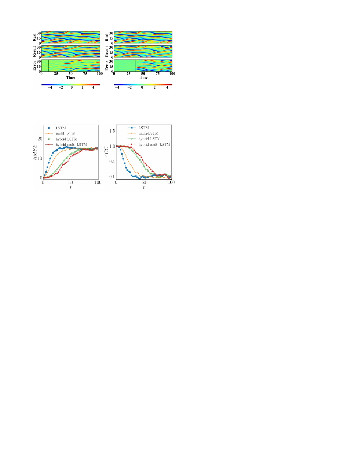
A hybrid model based on deep LSTM f or predicting hig h-dimen sional chaotic systems A hyb rid mo del based on deep LSTM fo r p redicting high-dimensional chaotic systems Y ouming Lei, 1, 2 , a ) Jian Hu, 1 and Jianpe ng Ding 1 1) Scho ol of mathematics and statistics, Northwestern P olytechnical University , Xi ’an 71007 2, China 2) MIIT Ke y Laboratory of Dynamics and Contro l of Complex Systems, Northwestern P olytech nical University , X i’an 710072, China (Dated: 4 F ebruary 2020) W e propo se a hyb rid m e thod combining th e deep long sho rt-term memory (L ST M) model with th e inexact emp irical model of dynamical systems to predict high-d imensional chaotic systems. The deep hierarchy is en coded into the LSTM by superimp osing multiple recu rrent n eural n e twork lay ers an d the hyb rid model is traine d with the Adam optimizatio n algorithm . The statistical r esults of the Mackey-Glass system a n d the Kura m oto-Siv ashinsky system are obta in ed under the criter ia o f root mean square er ror (RMSE) and anomaly correlation coefficient (ACC) using the sing e-layer LSTM, the multi-layer LSTM, an d the c o rrespon ding hybrid method, respectively . The numerica l r esults show that the prop osed m e thod can effecti vely a void the rapid di vergence o f the multi-layer LSTM model when reconstructin g chaotic attracto r s, a n d d e m onstrate the fe asibility of the co mbination of d eep learnin g based on the g radient descen t method and the em pirical mo del. It is difficult to predict long -term behaviors o f chaotic sys- tems o nly with an inex act empirica l mathemat ica l model because of t heir sensitivity on in itia l conditions. However , data-driven pr edictio n has made great progress in recent years with t he reserv oir co mputing (RC) , one o f two well- known kinds o f recurrent neural network, whose predic- tion performance is much bett er than various prediction methods such a s the dela yed phase space reconstruction. The long short-term memory , as the other kind of recur - rent neural network, has the ability to extract the tempo- ral structure o f dat a . Similar t o feedforward neural net- work in str ucture, it can be easily transformed into a deep one, which is very extensive in practica l applicatio ns. In this paper , we combine the deep LSTM model with the empirical model of the system to improve the prediction performance significantly with great po tential. I. INTRODUCTION The predictio n of chao tic systems is o ne of the mo st impo r- tant research fields in recen t y ears. It h a s been widely used in geolog ical science, m eteorolog ical prediction , signal pr o- cessing and industrial au tomation. Because of the sensiti vity on initial values and the co m plex fractal structur e of ch aotic systems, the establishmen t of a pred iction mode l is a chal- lenging task. At present, this task is mainly accomplished in two ways. One is th at over the years, many scientists have es- tablished mechan ism mo dels su ch as differential eq uations b y analyzing the internal laws and simp lifying main characteris- tics o f natural sy stems. The o ther is a d ata-driven forecast- ing m ethod, wh ich uses kno wn d ata sets to build "black box" prediction m o dels. The f ormer requ ires a lot of expert knowl- edge. Because of a lack of knowledge on re ality systems, the a) Electroni c mail: leiyouming@nwpu.ed u.cn. mechanism models have to neglect min or details an d are usu- ally ap proxim ate. Therefore, it is difficult for chaotic systems to achieve reliable long-ter m pred iction. The ad vantage o f the latter is that it only needs collection o f data, regardless of the inherent complex dy namics. B ut data from reality systems up- date quickly in the info rmation age nowadays and are difficult to collect on time without erro rs. There is not an omnipo - tent data-based model to pred ict all of th e sy stem s since data driven mod e ls lack theo retical supp o rts an d req u ire tun in g pa- rameters in ter ms of specific prob lems. In 2018, Pathak proposed a new hybrid method based on Reserver Compu ting (RC), which uses the advantages of data and system dynam ic structur e, and pointed out that this method is also a p plicable to other machine learnin g models 1 . In fact, both the RC an d the LSTM model are derived from general recu r rent neural networks. In 200 1, Maass and Jaeger propo sed a reser ve p ool calculation fo r cyclic n eural network, respectively , which ran domly determines th e cyclic hidd en unit, so that it could well cap tu re the input history of the sequence in the past, an d only lear ns the outpu t weight, re- ferred to as RC 2–4 . It was intr o duced to pred ict the trajec- tories of cha otic systems with g ood effects 5–11 . The LSTM, on th e other han d, is a path that introd uces self-cir c u lation to prod u ce gradient continuous flo w for a lo ng time 12,13 . As early as 2 002, relev ant studies ha ve app lied the LSTM model to chaotic system pred iction, but the ef fect was not ideal be- cause of the lack of technology a t that time 14 . Subsequently , numero us stud ies on data-driv en LSTM prediction of ch aotic systems have em erged 15 ,16 . In 2017, a dee p learning n etwork for chao tic system pr ediction b ased on noise ob servation was propo sed 17 , and the LST M model was u sed to filter o ut noise effecti vely , and th e cond itio nal proba b ility distribution of p re- dicted state variables was realized . In 2018 , Vlachas et a l. applied LSTM to the p rediction of h ig h-dimen sional ch aotic systems, and pr oved the f easibility of LSTM to pred ic t chaotic systems by comparin g it with the GPR me th od. They also pointed out tha t LSTM has the poten tial to mix with other methods to better prediction perf ormanc e 18 . In 2018, W an et A hybrid mo del based on deep LSTM f or predicting h ig h-dimen sional cha o tic systems 2 al. combined L STM with th e system’ s reduc ed or der equa- tion to pred ict the nonlinear part of systems and the extreme ev ent of complex d y namic eq uations 19 . The mo deling o f time series by RNN ca n captur e the fast and slow c h anges o f the system, and their un derlying co mponen ts are o ften composed in a lay ered way . In 199 5, Hihi and Bengio prop osed th at the d eep RNN structure could help extend th e ability of RNN to simulate th e long-ter m d ependen cies of d ata. They showed th at the depen- dencies of different time scales could be easily and effectiv ely captured by explicitly di viding the hidden units of RNN into group s c orrespon ding to dif feren t scales 20 . Curren tly , a com- mon method to enco de this hierarch y into RNN is to super- impose multiple cyclic neural netw or k laye rs 21–23 . There ar e many variations and im p rovements of the deep RNN struc- ture model based on the sup e r position le vel. For examp le, in 2015, Chung et a l. proposed a gated feedfor ward RNN based on deep LSTM 24 . In 2 016, W an g et al. prop osed a regional CNN-LSTM model and applied it to text e m otion analysis 25 . The video caption dec oder was simulated by a CNN-LSTM model c o mbined with atten tio n mech anism in 201 7 26 . T o pre- dict ch aotic systems mor e effecti vely , this work aims to ex- plore the feasibility o f c ombinin g the deep long sho rt-term memory (LSTM) model, which is based on the gradien t de- scent method , and the empirical model. In practice, we can use all of the resourc e s, data and prer equisite knowledge, and combine them to ach iev e an op timal pred iction result. The r est of the paper is as fo llows. In Sec.II, we introduce the structure o f the h ybrid m ethod b ased on the mu lti- layer LSTM model, and describe in detail the training pr o cess an d prediction process of the meth od. In Sec.III, we presen t thr e e common ly used measures to compar e th e d ifferences between the single-laye r LSTM mod el, the multi-lay e r LSTM mod el, and the h ybrid prediction method . In Sec.IV, we demon- strate the fe a sib ility of the hyb rid meth od based on the mu lti- layer LST M model in the Mackey-Glass system a n d in the Kuramoto-Sivas hin sky system, respectiv ely . Conclusions are drawn in Sec. V . II. HYBRID METHOD W e consider a d ynamical system who se state variable x ( t ) ∈ R d is a vailable in th e p ast tim e . For recurrent neur al network (RNN), given input sample x = ( x 1 , . . . , x T ) , its hid den vector is h = ( h 1 , . . . , h T ) and the input vector satisfies update eq u a- tions as fo llows,  h t = ϕ ( W xh x t + W hh h t − 1 + b h ) , y t = W hy h t + b y , (1) where W and b represent the weig h t matrix and the b ias vector, and ϕ is th e function o f th e hidd en layer . In add ition to the external circu lation of the neu r al n etwork, LSTM also has an intern al "self-loo p", shown in Fig. 1. For the LSTM model, ϕ is gener ally realized by the following FIG. 1. The structure of the "cell" in the LSTM model. FIG. 2. Sample diagram of the deep LSTM model. composite f unction,              i t = σ ( W xi x t + W hi h t − 1 + b i ) , f t = σ ( W x f x t + W h f h t − 1 + b f ) , o t = σ ( W xo x t + W ho h t − 1 + b o ) , c t = f t c t − 1 + i t tanh ( W xc x t + W hc h t − 1 + b c ) , h t = o t tanh ( c t ) , (2) where σ is the sigmo id function , g f t , g i t , g o t ∈ R d h × ( d h + d i ) repre- sent the forget, input, a n d outp ut gates respectively , c , h ∈ R d h are the "cell" state and the hidden state, W x i , W x f , W x o , W x c ∈ R d h × d i , W h i , W h f , W h o , W x c ∈ R d h × d h are train ing weights, and b i , b f , b o , b c ∈ R d h are biases. The LST M hid den and cell states ( h t and C t ) are called LSTM states jointly , the dimen- sion of these states is the number of hidden units d h , which controls th e ab ility of cells to learn historical data. The process of predicting chaotic system by multi- la y er LSTM is shown in Fig. 2. Consider a dynamic system, the time series data f rom the system D = { x 0: N t } are k nown, where x t ∈ R d i is the system state at time step t . The pro- cess of f u lly pred icting its state variables by the multi-layer LSTM model is di vid ed into two stages: train ing an d p r edic- tion. Durin g the training process, the training set is processed into samples in the c orrespon ding f orms of th e input and out- A hybrid mo del based on deep LSTM f or predicting h ig h-dimen sional cha o tic systems 3 put of th e mu lti-layer LST M mo d el, x t rain t =     x t + d − 1 x t + d − 2 . . . x t     , y t rain t = x t + d , (3) for t ∈ { 1 , 2 , . . . , N t rain − d + 1 } . These tra in ing samples used to optimize th e m odel parameter s to satisfy the m apping r e- lation of x t → y t . The deep architectur e learn in g mo del can build a higher level interpretation of attrac to rs. For the spe- cial stru cture of LSTM, the deep RNN c an be constructed by superimpo sing several hid den layers ea sily , where the output sequence of each layer is taken as the input sequence of the next layer, as shown in Fig . 2. For the deep RNN co nstructed by the N-la y er LSTM model, th e same hid den function is used for all layers in the stack, then the iterati ve calculation equa- tion of h idden layer sequ ence h n of the n -th layer is as follows, h n t = ϕ ( W h n − 1 h n h n − 1 t + W h n h n h n t − 1 + b n h ) , (4) where, n = 1 , 2 , ..., N , t = 1 , 2 , ..., T an d h 0 = x , the o utput y t is, y t = W h N y h N t . (5) The loss f unction of each sample is, L ( x t rain t , y t rain t , w ) =   F w ( x t rain t ) − y t rain t   2 , (6) where F w ( x t rain t ) r epresents the outpu t of th e mo del. In th e actual tr a ining pr ocess, to pr ev ent overfitting, regularization terms are a d ded into the err or , an d the to tal error functio n is defined a s, L ( D , w ) = 1 S S ∑ b = 1 L ( x t rain b , y t rain b , w ) + λ ∑ ω ∈ W T k ω k 2 , (7) where S = N t rain − d + 1 is the total numb er of the training samples, and W T is the set of all trainable parame te r m etrices. For N = 1, the mo del degrad e s to a single-lay er LSTM mo d el. At p resent, deep lea r ning combin ed with th e empir ical model was rarely used to predict chaotic systems, and an ef- fective hyb rid method based on the reservoir computing was propo sed 1 . Follo wing it, the structu r e of comb ining the multi- layer L STM model and th e em pirical mod el is shown in Fig. 3. During th e training p hase, th e training data samples firstly flow into the empirical m odel to get the empirical d a ta , then flow thro ugh the in put layer in to the multi-lay e r LSTM m odel with the em pirical d ata together, an d the outp ut of the model and the e m pirical data fin ally flow thr ough the o utput lay er to obtain the pred iction result. In the pred iction phase, the in p ut data is gradually replaced b y the pr ediction re sults, an d the prediction time is iterated until the e rror reaches th e thresh- old value for the first time. W e assume th at the em pirical model is an inaccur a te dif fer ential equation of the dyn a mical system, whose inacc u racy is r epresented by par ameter mis- match with a small err or ε . Alth ough the em pirical m o del only slightly cha nges system parameter s, this can, without FIG. 3. The hybrid meth od based on multi-layer LSTM, combined the deep LSTM model with the empirical model. loss of generality , gene rate large errors in an unkn own way , which makes long-term prediction impossible only using the mismatch model. I n fact, we can c o nsider the param eter m is- match ε comes from an inevitable error in constru c tin g dy- namical equations based on co gnitive mo dels. In this c a se, assume that the state variables in the d y namical system at the previous position are kn own, and the following state variables can be ob tained by integrating the em p irical model, so we have u ( ε ) t + ∆ t = E [ u ( t )] ≈ u ( t + ∆ t ) . (8) Then the samp le pairs o f the h ybrid method b a sed on multi- layer LSTM ar e as fo llows, x t rain t =     [ x t + d − 1 , E ( x t + d − 1 )] [ x t + d − 2 , E ( x t + d − 2 )] . . . [ x t , E ( x t )]     , y t rain t = x t + d , (9) where t ∈ { 1 , 2 , . . . , N t rain − d + 1 } , [ · , · ] repr esents th e splicing of vectors. If a = [ a 1 , a 2 , · · · , a m ] T , b = [ b 1 , b 2 , · · · , b n ] T , [ a , b ] is [ a 1 , a 2 , · · · , a m , b 1 , b 2 , · · · , b n ] T . the core pa rt o f th e mo del is stacked with multi-layer LSTM as men tioned above, and the output of th e mo del is chang ed to, y t = W h N y h N t + W e y E ( x ( t + d − 1 )) . (10) In this work, the same tra in ing method is u sed for differ- ent models when c omparin g the pr e d ictiv e power of different models. In the a c tu al training pro cess, the me th od of small batch gr a dient descen t is used to so lve the optimal par ame- ters. The sam ples are fe d into th e model in batches, and the loss fu nction is defined as the mean of the sample loss function for each batch. Th e trainin g weights are first initialized with Xavier a n d then iter ati vely op tim ized for the n etwork weights. The gradient descen t op timizer is used as, w i + 1 = w i − η ∇ w L ( x t rain t , y t rain t , w i ) , (11) where η is th e learnin g rate, W i is th e weight parameter o f batch i th befo re o ptimization, an d W i + 1 is the upda ted we ig ht parameter . According to different systems, the optimizer s used ar e different. In order to prevent th e parameter co n - vergence to a local optimal solution , w e use the Adam op ti- mizer, wh ich takes the first and secon d moment estimation o f A hybrid mo del based on deep LSTM f or predicting h ig h-dimen sional cha o tic systems 4 FIG. 4. The process flow chart of the hybrid multi-layer LSTM model combined with the empirical model. the gradient into accou nt to accelerate the training speed and effecti vely a void the mod el conv ergenc e to the lo c al optima l solution. The updated equatio n s are w r itten as, g = ∇ w L ( x t rain t , y t rain t , w i ) , m i + 1 1 = β 1 m i 1 + ( 1 − β 1 ) g , m i + 1 2 = β 2 m i 2 + ( 1 − β 2 ) g 2 , ˆ m 1 = m i + 1 1 / ( 1 − β i 1 ) , ˆ m 2 = m i + 1 2 / ( 1 − β i 2 ) , w i + 1 = w i − η ˆ m 1 / ( √ ˆ m 2 + ε ) . (12) After each epoch , we u p date the lear n ing rate b y η = γ × η , so that the model r emains stable after sev eral tr aining ses- sions. In order to make the mode l lear n d a ta featur es more fully , the training samples are nor malized d uring the train- ing process. In the pr ediction pr ocess, the tra in results of the model are reversed-normalized an d taken as the inpu t data in the next step. Th e co mplete flow chart is shown in Fig. 4. Here, u 1 , u 2 , ..., u d are the real data of the dy namical system, which are in put into th e empirical mo del E to g et ˜ u 1 , ˜ u 2 , ..., ˜ u d . Normalize them in P , and then input the processed data into the multi-laye r LSTM mod el ab ove. After that, input th e out- put result  h N d , ˜ v d + 1  into the full conne ction lay er , an d th u s get the pred icted value u F d + 1 . In the next step , u p date the input to u 2 , u 3 , ..., u F d + 1 , and get the correspond ing prediction u F d + 2 . Repeat th is p rogress u ntil we g e t the final result. II I. BENCHMARKS W e ado pt three commonly measures, the norm alized erro r, the r oot mean square e r ror (RMSE), an d the anom a ly co rrela- tion co efficient (A CC), to co mpare the pr ediction per forman ce of different models: singer-layer LSTM, multi-layer LSTM, hybrid singer-layer LSTM, and hybrid multi-layer LSTM. Considering th e dimensionless proper ty of the mod el, we r efer to th e time un it as the Model T ime ( M T ), which is the produ ct of th e time step and the num ber of iteration steps. T he nor- malized error E x p ( t ) for each in depend ent prediction p rocess is d efined as, E x p ( t ) = k x ( t ) − ˜ x ( t ) k D k x ( t ) k 2 E 1 / 2 , (13) where x ( t ) is the real d ata o f the chao tic system, an d ˜ x ( t ) is the predictio n result of the mo del. E ach method ev aluates the effecti ve time by several inde p endent pred icti ve experiments. The effecti ve time t v is de fin ed as the first time that the nor- malized error of the pre d iction mo d el reac hes the thr eshold value f , 0 < f < 1. The RMSE is defined as, RM S E t = r 1 V ∑ V i = 1    x ( i ) t − ˜ x ( i ) t    2 , (14) where V refers to the numb er of different p r ediction position s selected. In the fo llowing, V = 100. In addition, we used the mean ano m aly correlation coefficient ( ACC), wh ich is a widely used prediction accuracy index in the meteorolog ical field, at the pred icted location to quantify the correlation be- tween the predicted trajectory and the real on e. The ACC is defined a s, A CC t = V ∑ i = 1 ( x ( i ) t − ¯ x ) T ( ˜ x ( i ) t − ¯ x ) s V ∑ i = 1    x ( i ) t − ¯ x    2 s V ∑ i = 1    ˜ x ( i ) t − ¯ x    2 , (15) where ¯ x is the mean value of the trainin g d ata, and x ( i ) t and ˜ x ( i ) t represent the predic ted an d true values of the track at the time of t for the position o f i -th. The value r ange o f AC C is [ − 1 , 1 ] , and the m aximum value is 1 while the pred icted tra je c to ry and true value ch ange are con sistent com p letely . IV. RESUL TS In th is sectio n , different prediction mo dels are ap plied to two classical chaotic systems: the Mackey-Glass ( M G) sys- tem an d th e Kuramo to-Siv ashinsky (KS) system. A. The Macke y-Glass mo del The MG system is a typical time-delaye d chaotic system, and the e q uation is, ˙ x t = β x t − τ 1 + x n t − τ − γ x t , (16) where β = 2 . 0 , γ = 1 . 0 , n = 9 . 65, x t − τ is the d elay term, and τ = 2 represen ts the tim e de la y . For the MG system, we solve the equa tio n with a second-o r der Runge- Kutta algor ithm with a time step d t = 0 . 1 up to T = 10000 steps, and recon struct the phase space with the data. The em bedded dimension is 8 , and the time d elay is 0 . 1 to obtain the training d ata set. Based on the real MG system, the empirical model ap p roximate ly constructs the chaotic attractor by chan g ing γ in Eq . (16) to γ ( 1 + ε ) . The erro r variable ε is the dimen sionless difference between the empirical model and the real model, ε = 0 . 05. For the hyb rid meth o d b ased on the multi-layer LSTM, the attractor can be rec onstructed by trainin g da ta a nd labels. W e construct the d e ep LSTM mo del with N = 5, and th e label A hybrid mo del based on deep LSTM f or predicting h ig h-dimen sional cha o tic systems 5 T ABLE I. T he parameters for predicting t he MG system. Parameter V alue Parameter V alue ba t ch 20 η 0 . 001 d 21 γ 0 . 95 d h 40 λ 5 × 10 − 6 FIG. 5. (Color online) Sample diagram of predicting the MG system, (a)the multi-l ayer LST M model; (b)the hybrid model based on multi- layer LSTM. is given as y t rain = x t + d − x t + d − 1 . The em p irical model d ata could b e ob tained b y , E ( x t ) = d t × ˙ x ( ε ) t , (17) ˙ x ( ε ) t = β x t − τ 1 + x n t − τ − γ ( 1 + ε ) x t . (18) These data are reused for e poch = 150 time s, and bat ch sam- ple pairs are fed for each e poch . The hidd en d imension o f LSTM is d h , and the truncation len g th of error back propa- gation is d . Parameters of the mode l are shown in T abel I, Figure 5 shows the predictio n r esult. Th e error thresho ld is f = 0 . 1, an d the blue dotted line is the real data of the MG system. The predictio n time of the hybr id meth od based on multi-layer LST M reac h es 89 . 95 M T , which is significantly improved com pared with the pred ictio n time 33 . 02 M T of the multi-layer LSTM mo del. Further, the statistical erro r for pre- dicting 100 different location by f our m ethods above with th e same train ing d ata is shown in Fig. 6, where th e abscissa is forecast time, an d the ordina te is the mean of the roo t mean square error (RMSE) an d the mean of anom aly correlatoin coefficient (AC C), respectively . Under the ev aluation crite- ria, the pred iction perf ormanc e can be sorted as: single-lay er LSTM < m ulti-layer LSTM < hy brid single-layer LSTM < hybrid mu lti-layer LST M . B. The Kuramoto-Sivashinsky model The KS system is widely used in many scientific fields to simulate large-scale chaotic physical systems, which is d e- duced by Kuramoto o riginally 27 ,28 . Th e one-dimensio n al KS FIG. 6. (Color online) T he statisti cal error for predicting the MG system using four models (single-layer LSTM, multi-layer LSTM, hybrid single-layer L STM and hybrid multi- l ayer LSTM). T ABLE II. T he parameters for predicting the KS system. Parameter V alue Parameter V alue ba t ch 100 η 0 . 001 d 20 γ 0 . 98 d h 50 λ 5 × 10 − 10 system with in itial con ditions an d boun dary is given by , ∂ u ∂ t = − v ∂ 4 u ∂ x 4 − ∂ 2 u ∂ x 2 − u ∂ u ∂ x , (19) u ( 0 , t ) = u ( L , t ) = ∂ u ∂ x     x = 0 = ∂ u ∂ x     x = L = 0 . (20) In ord er to obtain the real data, discr e tization via a secon d- order differences schem e y ie ld s, d u i d t = − v u i − 2 − 4 u i − 1 + 6 u i − 4 u i + 1 + u i + 2 ∆ x 4 − u i + 1 − 2 u i + u i − 1 ∆ x 2 − u 2 i + 1 − u 2 i − 1 4 ∆ x , (21) where L = 35 is the perio dicity length , the grid size has D = 6 5 grid points, and the samplin g tim e is d t = 0 . 25. The approxi- mate e m pirical mo del is E ( u t ) = u ( ε ) t + 1 , (22) ∂ u ( ε ) ∂ t = − v ∂ 4 u ∂ x 4 − ( 1 + ε ) ∂ 2 u ∂ x 2 − u ∂ u ∂ x , (23) where ε = 0 . 0 5. W e use the data of T = 25000 to tr ain the model with e p och = 15 0, and the par ameters ar e shown in T able II. Figure 7 shows the prediction results of the chao tic attrac- tor in the KS system with the multi-lay er LSTM model and the hybrid mu lti-layer LSTM mod el. In the left figure, gi ven the er ror threshold o f f = 0 . 4, the predic tio n effecti ve tim e of the mu lti-layer LSTM model is 12 . 11 M T , wh ile the pre- diction time of the hybrid mo del c ombined with the em pirical model is improved to 38 . 04 M T . Fur ther , the statistical error for pred icting 1 00 d ifferent locations with four meth ods ab ove with the same training data is shown in Fig. 8, where the ab- scissa is forecast time, and the or dinate is the mean of the root A hybrid mo del based on deep LSTM f or predicting h ig h-dimen sional cha o tic systems 6 FIG. 7. (Color online) Sample diagram of predicting the KS system, (a)the multi-l ayer LST M model; (b)the hybrid model based on multi- layer LSTM. FIG. 8. (Color online) T he statisti cal error for predicting the MG system using four models (single-layer LSTM, multi-l ayer LSTM, hybrid single-layer L STM and hybrid multi- l ayer LSTM). mean square er ror (RMSE) and the m e a n o f an omaly co rrela- toin coefficient (A CC), respectively . Under the evaluation cri- teria, the predictio n performan ce can be sorted as: sing le-layer LSTM < m ulti-layer LSTM < hy brid single-layer LSTM < hybrid multi-layer LSTM. The above n umerical results show that for high dimensional chaotic stran ge attra c tors, in c reas- ing the depth of LSTM model can better the p rediction p er- forman ce to some extent. The hybrid metho d b ased o n the multi-layer LSTM has sign ificantly improved the pred iction capability , which means that the introd uction of the empir ical model pro m otes the d eep learning meth od b ased on the g radi- ent d escent m ethod. V. CONCLUSION In th is pap er , we pro pose a hybr id method based on the deep LSTM with mu lti- la y ers to predict chaos in the MG sy stem and in the KS system , r espectively . The L ST M model h as a flexible structur e and its successful comb ination with the inex- act empirical m odel provid es a feasible way to the pr ediction of high-dim ensional chao s. W e can give a heur istic e xp lana- tion. The data d r iv en LSTM mod el can capture loc a l charac- teristics of a cha otic attractor and thus accur ately predict the short-term behavior of the system. With time ev olu tion, the div ergen cy o f the deep LSTM model fro m the true trajectory is u nav oidab le wh en reco n structing the c h aotic attracto r . This makes lo ng-term prediction dif ficult to implement. Introd uc- ing the em pirical mod el is just like to tell th e hybr id mo del "climate" of the cha o tic attractor so th at the deviance between the trajectory an d its prediction is corrected to som e extent. In this way , co mbining th e deep LSTM model with the em- pirical model improves th e capability of the hyb rid model to capture the steady- state behavior o f th e chaotic attractor while keeping the ability o f short-term predictio n. Note that the prediction performance of the hybrid model based on the deep LSTM is much bett er than the scheme of RC, while it is similar to the hybrid model combined RC and the em- pirical model alt hough its tra ining co st is higher than the latter . Ma ybe her e we have not fully harness th e power of the structure o f the LSTM. Futu re w ork can focus on h ow to improve th e perfor mance of the h ybrid model based on a the- oretical understan ding o f th e advantage of the LSTM. VI. ACKN OWLEDGEMENT This work was supp orted by the Natio nal Natural Scienc e Foundation of China (Grant No. 11672 231) and the NSF of Shaanxi Provin ce (Gran t No. 201 6JM1010 ). 1 J. Path ak, A. Wikne r, R. Fussell, S. Chandra, B. R. Hunt, M. Girv an, and E. Ott, “Hybri d forecastin g of chaotic processes: Using machine learning in conjunc tion with a knowl edge-based model, ” Chaos: An Interdisci plinary Journal of Nonlinea r Science 28 , 041101 (2018). 2 W . Maass, T . Natschläg er , and H. Markram, “Fading memory and kernel properti es of generic cortical microcirc uit models, ” Journal of Physiology- Paris 98 , 315–330 (2004). 3 H. Jaege r, “Echo state network , ” Scholarpe dia 2 , 2330 (2007). 4 H. Jaege r and H. Haas, “ Harnessing non linearity: Predicting chaotic sys- tems and sa ving ene rgy in wirele ss communicati on, ” Science 304 , 78–80 (2004). 5 Z. Lu, J. Pathak , B. Hunt , M. Girvan , R. Brocket t, and E. Ott, “Rese r- voir observers: Model-free inferenc e of unmeasure d va riables in chaotic systems, ” Chaos: An Interd isciplinary Journal of Nonlinear Scienc e 27 , 041102 (2017). 6 J. Pathak, Z . Lu, B. R. Hunt, M. Girvan, and E. Ott, “Using machine learn- ing to replica te chaot ic attrac tors and calculate lyapuno v exponent s from data, ” Chaos: An Int erdisciplina ry Journal of Nonlin ear Scienc e 27 , 121102 (2017). 7 Z. Lu, B. R. Hunt, and E. Ott, “ Attractor reconstruct ion by machine learn- ing, ” Chaos: An Interdiscipli nary Journal of Nonlinear Science 28 , 061104 (2018). 8 D. Ibáñez-Sori a, J. Garcia-Ojalv o, A. Soria-Frisch, and G. Ruf fini, “Detec- tion of generalize d synchronizat ion using echo s tate network s, ” Chaos: An Interdisc iplinary Journal of Nonlinear Science 28 , 033118 (2018). 9 K. Nakai and Y . S aiki, “Machin e-learning inference of fluid v ariables from data using reservoi r computing, ” Physical Re view E 98 , 023111 (2018). 10 P . Antonik, M. Gulina, J. Pauwels, and S. Massar , “Using a reserv oir com- puter to learn chaotic attract ors, with applicati ons to chaos synchroniz ation and cryptography , ” Physical Revie w E 98 , 012215 (2018). 11 J. Patha k, B. Hunt, M. Girvan, Z. Lu, and E. Ott, “Model-fr ee prediction of larg e spat iotemporally cha otic systems from data: A rese rvoir computing approac h, ” Physical Re view Letters 120 , 024102 (2018). 12 S. Hochrei ter and J. Schmidhuber , “Long short-term memory , ” Neural Computati on 9 , 1735–1780 (1997). 13 F . Gers, J. Schmidhuber , and F . Cummins, “Learning to forget: continual predict ion with lstm, ” Neural Computation 12 , 2451 (2000). 14 F . A . Gers, D. Eck, and J. Schmidhuber , “Applying lstm to time series predict able through time-windo w approaches, ” in Neural Nets WIRN V ie tri- 01 (Springer , 2002) pp. 193–200. 15 S. Brunton, B. Noack, and P . Ko umoutsakos, “Machine learni ng for fluid mechanic s, ” arXi v preprint arXi v:1905.11075 (2019). 16 S. Lahmiri and S. Bekiros, “Cryptocurre ncy forecasting with deep learning chaoti c neural networks, ” Chaos, Solitons & Fractal s 118 , 35–40 (2019). A hybrid mo del based on deep LSTM f or predicting h ig h-dimen sional cha o tic systems 7 17 K. Y eo, “Model-f ree prediction of noisy chaotic time s eries by deep learn- ing, ” arXi v preprint arXi v:1710.01693 (2017). 18 P . R. Vlacha s, W . Byeon, Z. Y . W an, T . P . Sapsis, and P . Koumout sakos, “Data-d riv en forecasting of high-dimensi onal chaotic systems with long short-term memory networks, ” Proceedings of the Royal Society A: Math- ematica l, Physical and Engineering Sciences 474 , 20170844 (2018). 19 Z. Y . W an, P . Vlac has, P . K oumoutsakos, a nd T . Sapsis, “Data-assisted reduced -order modeling of extreme ev ents in complex dynamical systems, ” PloS One 13 , e0197704 (2018). 20 S. El Hihi and Y . Bengio, “Hierarchica l recurre nt neural networks for long- term depe ndencies, ” in Advanc es in Ne ural In formation Pr ocessing Sy stems (1996) pp. 493–499. 21 A. Grav es, “Generating sequences wi th recurrent neural networks, ” arXiv preprint arXi v:1308.0850 (2013). 22 J. Schmidhuber , “Learni ng complex, extende d s equences using the princi- ple of history compression, ” Neural Computation 4 , 234–242 (1992). 23 M. Hermans and B. Schrauwen, “Trai ning and analysing deep recurr ent neural networks, ” in Advances i n N eural In formation Pr ocessing Systems (2013) pp. 190–198. 24 J. Chung, C. Gulcehre, K. Cho, and Y . Bengio, “Gated feedback recurrent neural netw orks, ” in International Confer ence on Mac hine Learni ng (2015) pp. 2067–2075. 25 J. W ang, L .-C. Y u, K. R. Lai, and X. Zhang, “Dimensional sentiment anal- ysis using a re gional cnn-lstm model, ” in P r oceedings of the 54th Annual Meeti ng of the Association for C omputational Linguistic s (V olume 2: Short P aper s) (2016) pp. 225–230. 26 J. Song, Z. Guo, L. Gao, W . Liu, D. Zhang, and H. T . Shen, “Hierarc hical lstm with adjusted temporal attention for video captioning, ” arXiv preprint arXi v:1706.01231 (2017). 27 Y . Kuramoto and T . Tsuzuki, “Persistent propagatio n of conc entration wa ves in dissipati ve media far from thermal equilib rium, ” Progress of The- oretic al Physics 55 , 356–369 (1976). 28 Y . Kuramoto, “Di ffusion-i nduced chaos in reactio n systems, ” Prog ress of Theoretic al Physics Supplement 64 , 346–367 (1978).