Tensor-to-Vector Regression for Multi-channel Speech Enhancement based on Tensor-Train Network

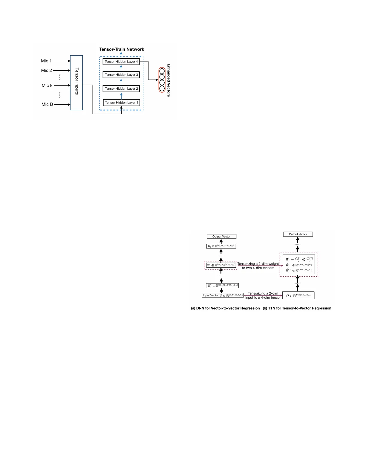
TENSOR-TO-VECT OR REGRESSION FOR MUL TI-CHANNEL SPEECH ENHANCEMENT B ASED ON TENSOR-TRAIN NETWORK J un Qi 1 ∗ , Hu Hu 1 ∗ , Y annan W ang 3 , Chao-Han Huck Y ang 1 , Sabato Mar co Siniscalchi 1 , 2 , Chin-Hui Lee 1 1 Electrical and Computer Engineering, Georgia Institute of T echnology , Atlanta, GA, USA 2 Computer Engineering School, Uni versity of Enna, Italy 3 T encent Media Lab, T encent Corporation, Shenzhen, Guangdong, China ABSTRA CT W e propose a tensor-to-v ector regression approach to multi-channel speech enhancement in order to address the issue of input size e x- plosion and hidden-layer size expansion. The ke y idea is to cast the con ventional deep neural network (DNN) based vector -to-vector regression formulation under a tensor -train network (TTN) frame- work. TTN is a recently emerged solution for compact represen- tation of deep models with fully connected hidden layers. Thus TTN maintains DNN’ s expressiv e power yet in volv es a much smaller amount of trainable parameters. Furthermore, TTN can handle a multi-dimensional tensor input by design, which exactly matches the desired setting in multi-channel speech enhancement. W e first provide a theoretical extension from DNN to TTN based regres- sion. Next, we show that TTN can attain speech enhancement qual- ity comparable with that for DNN but with much fewer parameters, e.g., a reduction from 27 million to only 5 million parameters is ob- served in a single-channel scenario. TTN also improves PESQ over DNN from 2.86 to 2.96 by slightly increasing the number of train- able parameters. Finally , in 8-channel conditions, a PESQ of 3.12 is achiev ed using 20 million parameters for TTN, whereas a DNN with 68 million parameters can only attain a PESQ of 3.06. Code is av ailable online 1 . Index T erms — T ensor-T rain network, speech enhancement, deep neural network, tensor -to-vector regression 1. INTR ODUCTION Deep neural network (DNN) based speech enhancement [1] has demonstrated state-of-the-art performances in a single-channel set- ting. It has also been e xtended to multi-channel speech enhancement with similar high-quality enhanced speech [2]. A recent overvie w can be found in [3]. In essence, the process can be abstracted as a vector -to-vector regression based on deep architectures with a DNN aiming at learning a functional relationship f : Y → X such that input noisy speech y ∈ Y can be mapped to corresponding clean speech x ∈ X . Se veral variants of deep learning structures have also been attempted, e.g., recurrent neural networks (RNNs) with long short term memory (LSTM) gates were employed in [4, 5]. A deep bidirectional RNN with LSTM gates was instead used in [6]. Moreov er, a generati ve adv ersarial network (GAN) was used in [7]. Spatial information can complement spectral information for improv ed speech enhancement lev eraging multi-channel informa- tion in more complex scenarios, where the sources of distortions include ambient noises, room re verberation and interfering speakers, * Refers to an equal contribution. 1 https://github .com/uwjunqi/T ensor-T rain-Neural-Network Fig. 1 . Con ventional multi-channel DNN-based vector-to-vector r e- gr ession for speech enhancement. as discussed in [8, 9, 10, 11], for example. Howe ver , the DNN-based vector -to-vector regression, which is the focus in this work, mainly aims at single-channel speech enhancement and is not simply gener- alized to multi-channel speech enhancement. As shown in Figure 1, a traditional approach to dealing with an array of microphones is ex- ploited spatial information at the input le vel by concatenating speech vectors from multiple microphones into a single high dimensional vector , e.g., [12, 2]. Thus the vector -to-vector re gression approach can still be emplo yed for speech enhancement by appending multi- channel feature vectors together into a high-dimensional vector and mapping it to a vector e xtracted from the reference v ector . Such a simple solution, unfortunately , clashes with our theoretical analysis outlined in [13], which suggests that the width of each hidden layer in a DNN needs to be greater than the input dimension plus two so that the expressi ve po wer of DNN-based vector -to-vector regression can be guaranteed. Moreover , high dimensional input vectors result in wider hidden non-linear layers, which in turn implies the need for huge computational resources and storage cost. Se veral proposals were put forth by different groups to ov ercome such an issue, for ex- ample, sparseness in DNN w as explored in [14] to reduce the model size; howe ver , the optimum implementation heavily depends on the specific hardware architecture. In [15], a singular value decomposi- tion approach was de vised, which is performed in a post-processing phase, that is, a DNN with a huge amount of parameters is first trained, and parameter reduction is then applied. In this work, we proposed to address the multi-channel speech enhancement problem within a more principled parameter reduction framew ork, namely the T ensor-T rain Network (TTN) [16], which does not require a multi-stage approach. A T ensor-T rain refers to a compact tensor representation of the fully-connected hidden lay- ers in a DNN [16]. In doing so, we put forth a tensor-to-vector Fig. 2 . A TTN-based speech enhancement system. regression approach that can handle multi-channel information and meanwhile addresses the issue of input size explosion and hidden- layer size e xpansion. As sho wn in Figure 2, the feature v ectors of B microphones are transformed into a tensor representation, such that the DNN-based vector -to-vector re gression can be reshaped to a TTN based tensor-to-vector mapping. W e show how the theorem on e xpressive power of the traditional DNN-based vector -to-vector [13] can be extended to be v alid in the TTN frame work. Next, we ev aluate our approach with both single- and multi-microphone ex- perimental setups, where the speech signal is exposed to multiple sources of distortions, including ambient noises, room re verberation and interfering speakers. W e show that TTNs can attain speech en- hancement quality comparable with DNNs, yet a 81% reduction in the size of parameters is observ ed, in the single-channel scenario. In 8-channel conditions, TTN deliv ers a PESQ of 3.12 using 20 million parameters. In contrast, a DNN-based multi-channel configuration needs up to 68 million parameters and attain a PESQ of 3.06. W e should also remark that T ensor-T rain decomposition can be applied to CNNs, and RNNs; howe ver , we focus on DNNs in this initial in- vestigation. The remainder of the paper is org anized as follows: Section 2 introduces TTN mathematical underpinnings and key properties. In Section 4, the experimental en vironment is first described, and then the experimental results are presented and discussed. Section 5 con- cludes our work. 2. TENSOR-TRAIN NETWORK TTN relies on a tensor-train decomposition [17] which can be described mathematically as follows: giv en a vector of ranks r = { r 1 , r 2 , ..., r K +1 } , tensor-train decomposes a tensor W ∈ R ( m 1 n 1 ) × ( m 2 n 2 ) ×···× ( m K n K ) , ∀ i ∈ { 1 , ..., K } , m i ∈ R + , n i ∈ R + into a multiplication of core tensors according to Eq. (1), where for the given ranks r k and r k +1 , the k -th core tensor C [ k ] ( r k , i k , j k , r k +1 ) ∈ R m k × n k in which i k ∈ { 1 , 2 , ..., m K } and j k ∈ { 1 , 2 , ..., n K } . Besides, r 1 and r K +1 are fixed to 1 . W (( i 1 , j 1 ) , ( i 2 , j 2 ) , ..., ( i K , j K )) = K Y k =1 C [ k ] ( r k , i k , j k , r k +1 ) (1) TTN is generated by applying the T ensor-T rain decomposition to the hidden layers of DNN. The ke y benefit from TTN is to sig- nificantly reduce the number of parameters of a feed-forward DNN with fully-connected hidden layers. It is because TTN only stores the TT -format of DNN, i.e., the set of low-rank core tensors { C k } K k =1 of the size P K k =1 m k n k r k r k +1 , which can approximately recon- struct the original DNN. In contrast, the memory storage of original DNN requires the size of Q K k =1 m k n k , which is much larger than P K k =1 m k n k r k r k +1 . Moreover , instead of decomposing a well- trained DNN into a TTN, core tensors can be randomly initialized and iteratively trained from scratch. Similar to the DNN training procedures, the optimization methods based on v ariants of stochas- tic gradient descent (SGD) can ensure con verged solutions. Besides, the work [16] shows that the running complexities of DNN and the corresponding TTN are in the same order scale. 3. TENSOR-TO-VECT OR REGRESSION The TTN framew ork offers a natural way to conv ert a speech en- hancement system from vector -to-vector to tensor-to-vector config- uration because multi-dimensional inputs can be directly fed into the TNN avoiding concatenating speech v ectors inputs into a single long vector . Figure 3 demonstrates a typical example of casting DNN- based vector -to-vector regression into a TTN-based tensor-to-v ector regression. More specifically , gi ven a list of ranks { r 1 , r 2 , r 3 } , the DNN input vector O ∈ R ( B 1 B 2 ) × ( Z 1 Z 2 ) is decomposed into a 4th order input tensors ˆ O ∈ R B 1 × B 2 × Z 1 × Z 2 before being used in the TTN-based configuration. Accordingly , the i -th weight matrix, W i , in the DNN is decomposed into a tensor product of two tensors ˆ W [1] i ∈ R r 1 × m i, 1 × n i, 1 × r 2 and ˆ W [2] i ∈ R r 2 × m i, 2 × n i, 2 × r 3 . The corresponding hidden layers with core tensors represent a basic ar- chitecture of TTN for tensor-to-v ector regression, and the output vectors of two architectures are set to be equal. Fig. 3 . T ransforming a DNN-based vector-to-vector re gr ession into a TTN-based tensor-to-vector r egr ession. T ensor-to-vector regression based on TTN can substantially re- duce the number of model parameters. Besides, we can pro ve that the TTN-based tensor-to-vector regression can maintain the repre- sentation power of the traditional DNN-based vector-to-v ector . Our theoretical work [13] on the representation power of DNN-based vector -to-vector regression suggests a tight upper bound to a numeri- cally estimate of the maximum mean squared estimation (MSE) loss. That MSE upper bound explicitly links the depth of ReLU-based hidden layers to the expressiv e capability of DNN models. More specifically , with input and out dimensions of d and q , respecti vely for a vector -to-vector regression target function ˆ f : R d → R q , there exists a DNN f DN N with K ( K ≥ 2) ReLU based hidden layers, where the width of each hidden layer is at least ( d + 2) and the top hidden layer has n K ( n K ≥ d + 2) units. Then, we can deri ve the equality of (b) in Eq. (2). || ˆ f − f T T N || 1 ( a ) ≤ || ˆ f − f DN N || 1 ( b ) = O ( q ( n K + K − 1) 2 ) (2) W e are currently dev eloping ne w theories on TTN-based tensor- to-vector mapping, which demonstrate that a TTN associated with the tensor decomposition of a DNN can keep the expressi ve power of DNN-based vector -to-vector re gression. Indeed, we can mathe- matically find a TTN f T T N representation such that the inequality of (a) in Eq. (2) is v alid. W e a void giving the proof of our new results here, but the experimental evidence given in the next section on the speech enhancement task supports our theoretical results in Eq. (2). The inequality in Eq. (2) is ensured to be valid under consis- tent training and testing en vironmental conditions. It basically states that a TTN has more expressiv e power than a DNN with a similar complexity . The detailed proof is shown in our another paper [18], and the effect is demonstrated in the e xperimental results in T ables 1 and 2 to be provided later . 4. EXPERIMENT AL SETUP & RESUL TS 4.1. Data Preparation The proposed TTN-based models are ev aluated on simulated data from WSJ0, which contains additive noise, interfering speakers, and rev erberation. The dataset is created by corrupting the WSJ0 cor- pus [19] with OSU- 100 -noise [20] data, allowing us to obtain 30 hours of training material, and 5 hours of testing data. When simu- lating the noisy data, each waveform is mixed with one kind of back- ground noise from the noise set. The target and additional interfering speech with their corresponding RIRs are conv olved to generate the final wav eform. In particular , our training and testing datasets are created from different noisy utterances of various speakers. As for the training dataset, a 5 -minute clean speech from each of the tar- geted speakers is randomly mixed with 73 interfering speakers and 90 types of additive noise. Each tar get an-echoic speech is generated by con volving clean speech with the direct path response between the target speakers and the reference channel. F or the testing dataset, another 5 -minute unseen speech of the target speakers is mix ed with 10 unseen interfering speakers and 10 types of unseen noise. The signal-to-interfered-noise-ratio (SINR) lev el of each utterance is set as follows: when SINR is 5 dB, the signal-to-noise-ratio (SNR) is configured to 10 dB or 15 dB; when SINR is 10 dB, the SNR is set to 15 dB; when SINR is 15 dB, the SNR is increased to 20 dB. The pro- portion of each SINR level is set equally . Besides, some utterances of SINR 30 dB are included in the training set to cover some very high SINR conditions. T o simulate rev erberated speech, a rev erberated acoustic envi- ronment is b uilt: A microphone array of 8 -circular channel micro- phone is arranged in a room of size 6 . 5 m × 5 . 5 m × 3 m in terms of length-width-height. As to the single-channel scenario, the mi- crophone is put at the center of the array . T o av oid unnecessary combinations of multiple interference, we deliberately constrain the conditions that the microphone array only aims at one target speaker , and it only receiv ed one kind of additive noise. Specifically , a hor- izontal distance of a tar get speak er to the center of the microphone array is strictly fixed to 3 m . Besides, we set both the target speaker and the interfering speaker keeping the same distance to the micro- phone array , and the angle of them is configured as 40 ◦ . Before we build the training and testing sets, an improv ed image-source method (ISM) [21] is used to generate RIRs of rev erberation time (R T 60 ) (from 0 . 2 s to 0 . 3 s ) and the corresponding direct path response for each microphone channel. For both training and testing datasets, the setting of RIRs is fixed to the same conditions, such as the room size, R T 60 , and all of the distances and directions. 4.2. Experiment Setting In our e xperiments, 257 -dimensional normalized log-po wer spectral (LPS) feature [22, 23, 24] is taken as the inputs to the DNNs. The LPS features are generated by computing 512 points Fourier trans- form on a speech segment of 32 milliseconds. For B -channel data, all channel inputs are concatenated together for the model training. For each input frame, the adjacent context of size M , is combined with the current frame. Hence, the size of the input for DNN is 257 × (2 M + 1) × B . For TTN, we ignore the first dimension of the input LPS features, which is the direct-current component. Thus, the input size for TTN is 256 × (2 M + 1) × B . After re gression, the first dimension of input is concatenated back to the 256 -dimension output without any change. The clean speech features of the first channel are assigned to the top layers of DNN and TTN, as the ref- erence during the training stage. Our baseline DNN model has 6 hidden layers, and each hidden layer is composed of 2048 neurons. The ReLU activ ation function is used for all hidden layers. A linear function is employed in the top hidden layer . As for the TTN, each hidden dense layer is decom- posed and replaced with a T ensor-T rain format, as shown in Figure 2. Both the DNN and TTN are trained from scratch based on the stan- dard back-propagation algorithm [25], and both models adopt the same training configuration. During the training phase, Adam opti- mizer is adopted, and the initial learning rate is set to 0 . 0002 . The mean square error (MSE) [26, 27] is used as the optimization object. The context window size at the input layer is set to 5 for all mod- els, in which the current frame is concatenated with the previous 5 frames and follo wing 5 frames (from the same channel). For both the DNN and TTN models, T ensorFlow [28] is used in all of our experiments. Perceptual ev aluation of speech quality (PESQ) [29] is used as our evaluation criterion. The PESQ score, which ranges from − 0 . 5 to 4 . 5 , is calculated by comparing the enhanced speech with the clean one. A higher PESQ score corresponds to a higher quality of the speech perception. 4.3. Single-channel Speech Enhancement Results The TTN framew ork is first ev aluated on the single-channel speech enhancement task. In T able 1, we can see that a 6 -layer DNN model, which is taken as a baseline system, achieves a PESQ score of 2 . 86 with 27 million parameters. A TTN architecture is generated by ap- plying tensor -train decomposition to the DNN baseline model. Each weight matrix of DNN is decomposed to two four-dimension ten- sors using tensor decomposition. For example, a weight matrix of the size 2048 × 2048 can be decomposed to two tensors with the size of 1 × 32 × 32 × 4 and 4 × 64 × 64 × 1 . The TTN core ten- sors are randomly initialized and then trained from scratch using the Adam optimizer [30]. As discussed in Sections 2 and 3, the forth row in T able 1 sho ws that a substantial parameter reduction when the T ensor-T rain format is employed. A drop in the PESQ value, from 2 . 86 (DNN) to 2 . 66 (TNN), is observed because of the parameter reduction. Nonethe- less, TTNs consistently deliv ers better and better speech enhance- ment results as its number of parameters increases. As shown in the seventh row in T able 1, the TTN model with 5 million parame- ters can achiev e nearly the same PESQ scores as the DNN baseline model ( 2 . 84 vs 2 . 86 ). Howev er , TTN model uses only 18% of the amount of parameters in the DNN, which suggests that TTN can sig- nificantly reduce the number of parameters while keeping the base- line performance. Furthermore, if we further increase the parameter number of the TTN model, we can even obtain a better TTN model achieving a 0 . 1 absolute PESQ improvement using only 74% of the DNN parameters, namely 20 million (see last row in the table). T able 1 . PESQ results for single-channel speech enhancement. Model Channel # Parameter # PESQ DNN 1 27M 2.86 DNN-SVD 1 5M 2.82 DNN-SVD 1 20M 2.84 TTN 1 0.6M 2.66 TTN 1 0.7M 2.71 TTN 1 2.6M 2.78 TTN 1 5M 2.84 TTN 1 20M 2.96 T o better appreciate the TTN technique, we have implemented the DNN-SVD method proposed in [15], which is a widely used post-processing compression technique for deep models. Each weight matrix in the trained DNN is first decomposed into two smaller matrix using SVD. The reduced size DNN is then fine-tuned with back-propagation. The DNN-SVD method can allow us to reduce the DNN size to 5 and 20 million parameters, as shown in the second and third rows in T able 1, respectively . Nonetheless, the PESQ drops to 2 . 82 with 5 million parameters. The PESQ attains a value of 2 . 84 when 20 million parameters are k ept after DNN-SVD, which is howe ver still lower than the PESQ attained by the original DNN. Most importantly , our TNN approach with 20 million param- eters attains a PESQ of of 2 . 96 , which not only compares fav ourably with the DNN-SVD solution with the same amount of parameters, but it represents an improvement over the DNN baseline approach, as already mentioned. 4.4. Multi-channel Speech Enhancement Results In this section, our inv estigation focuses on the microphone array scenario. The DNN-based multi-channel speech enhancement solu- tions realized in Figure 1 handles information from different mics at the input layer , which calls for wider input vectors and thereby an ov erall larger model size. By comparing the DNN baseline configu- ration in the first row in T ables 1 and 2, the parameter number goes from 27 million for the 1 -channel case to 33 million for 2 -channel case. In the 8 -channel case, the number of DNN parameters goes up to 68 million, as sho wn in the third ro w in T able 2. In multi-channel speech enhancement, the control of the size of the neural architec- ture therefore becomes even a more important aspect that cannot be ov erlooked. In the 2 -channel configuration, TNN parameters can be reduced to 0 . 6 million, but the PESQ would go do wn to 2 . 75 , as shown in the fourth row in T able 2. Ne vertheless, we can observe, by com- paring the first and sixth row in T able 2, that the TTN-based speech enhancement model can attain nearly the same performance of the DNN-based counterpart ( 3 . 00 vs. 2 . 96 ), while squeezing the num- ber of parameters from 33 million to 5 million. As in the single- channel case, DNN-SVD could be applied as a post-processing ap- proach for model compression, and it can achie ve a PESQ of 2 . 93 with 5 million parameters, as shown in the fifth ro w in T able 2. T able 2 . PESQ Results of Multi-channel Speech Enhancement Model Channel # Parameter # PESQ DNN 2 33M 3.00 DNN-SVD 2 5M 2.93 DNN 8 68M 3.06 DNN-SVD 8 5M 3.01 TTN 2 0.6M 2.75 TTN 2 5M 2.96 TTN 8 0.6M 2.83 TTN 8 5M 3.06 TTN 8 20M 3.12 In the 8 -channel configuration, the TNN model size can be signif- icantly reduced to 7% of the corresponding DNN size, namely from 68 million to 5 million, as shown in the eighth ro w in T able 2, while keeping the PESQ equal to 3 . 06 . When compared with the result of DNN-SVD method [15] reported in the fourth row in T able 2, although both DNN-SVD and TTN can reduce the model parame- ters to 5 million, the PESQ will decrease from 3 . 06 to 3 . 01 with the DNN-SVD method; whereas the TTN approach keeps the model performance. Such an empirical result demonstrates the adv antages in using a TTN-based tensor-to-vector regression approach to multi- channel speech enhancement and connects our theoretical analysis in Section 3. Furthermore, better speech enhancement results can be attained by increasing the TTN model size. Indeed, a TTN model with 20 million parameters, compared to the 68 million of the DNN baseline system, can achieve a PESQ of 3 . 12 , as shown in the last row in T able 2, which corresponds to a 0 . 6 absolute improvement ov er the DNN baseline solution. Since comple x noisy and re verberated conditions are in volv ed, the theory on the expressi ve power as sho wn in Eq. (2), is not strictly valid in our testing cases. But our improved theorems, which are to be published elsewhere and consider the generalization capability of models, can better correspond to our experimental results in T able 1 and 2. 5. CONCLUSIONS This work is concerned with multi-channel speech enhancement lev eraging upon TTN for tensor-to-vector regression. First, we describe the tensor-train decomposition, and its application to a DNN structure. Our theoretical results justify that the TTN-based tensor-to-v ector function allows fewer parameters to realize a higher expressi ve and generalization po wer of DNN-based v ector-to-vector regression. Then, we set up both single-channel and multi-channel speech enhancement systems based on TTN to verify our claims. When compared with DNN-based speech enhancement systems, ex- perimental e vidence shows that tensor-to-vector regression based on TTN compares fav orably with the DNN-based baseline counterpart in terms of PESQ, but it requires much fewer parameters. Fur- thermore, increasing number in the TTN-based configuration, we can achiev e better enhancement qualities in terms of PESQ, while amount of of parameters used in the TTN configuration is much less than the DNN counterpart. The related empirical results verify our theories and exhibit a potential usage of tensor-train decomposition in more adv anced deep learning models. Our future w ork will apply TTN decomposition to other deep models, such as recursi ve neural networks (RNNs) and con volution neural netw orks (CNNs). 6. REFERENCES [1] Y . Xu, J. Du, L.-R. Dai, and C.-H. Lee, “ A regression ap- proach to speech enhancement based on deep neural networks, ” IEEE/A CM T ransactions on Audio, Speec h and Language Pr o- cessing (T ASLP) , vol. 23, no. 1, pp. 7–19, 2015. [2] Q. W ang, S. W ang, F . Ge, C. W . Han, J. Lee, L. Guo, and C.-H. Lee, “T wo-stage enhancement of noisy and re verberant micro- phone array speech for automatic speech recognition systems trained with only clean speech, ” in ISCSLP , 2018, pp. 21–25. [3] D. W ang and J. Chen, “Supervised speech separation based on deep learning: An overvie w , ” IEEE/ACM T ransactions on Audio, Speech, and Langua ge Pr ocessing , v ol. 26, no. 10, pp. 1702–1726, 2018. [4] F . W eninger, H. Erdogan, S. W atanabe, E. V incent, J. Le Roux, J. R. Hershey , and B. Schuller , “Speech enhancement with lstm recurrent neural networks and its application to noise-robust asr , ” in International Conference on Latent V ariable Analysis and Signal Separation . Springer , 2015, pp. 91–99. [5] H. Zhao, S. Zarar , I. T ashev , and C.-H. Lee, “Con volutional- recurrent neural networks for speech enhancement, ” in IEEE International Confer ence on Acoustics, Speech, and Signal Pr ocessing (ICASSP) , 2018, pp. 2401–2405. [6] L. Sun, S. Kang, K. Li, and H. Meng, “V oice con version us- ing deep bidirectional long short-term memory based recurrent neural networks, ” in IEEE International Conference on Acous- tics, Speech, and Signal Pr ocessing (ICASSP) , 2015, pp. 4869– 4873. [7] S. Pascual, A. Bonafonte, and J. Serra, “Seg an: Speech en- hancement generative adversarial network, ” arXiv pr eprint arXiv:1703.09452 , 2017. [8] H. L. V an Trees, Optimum array pr ocessing: P art IV of detec- tion, estimation, and modulation theory , John W iley and Sons., 2004. [9] J. Benesty , J. Chen, and Y . Huang, Micr ophone array signal pr ocessing , JohSpringer Science and Business Media, 2008. [10] X. Xiao, S. W atanabe, H. Erdogan, L. Lu, J. Hershey , M. L. Seltzer G. Chen, Y . Zhang, M. Mandel, and D. Y u, “Deep beamforming networks for multi-channel speech recognition, ” in IEEE International Confer ence on Acoustics, Speech, and Signal Pr ocessing (ICASSP) , 2016, pp. 5745–5749. [11] Z. W ang and D. W ang, “ All-neural multi-channel speech en- hancement, ” in Interspeech . ISCA, 2018, pp. 3234–3238. [12] B. W u, M. Y ang, K. Li, Z. Huang, S.M. Siniscalchi, T . W ang, and C.-H. Lee, “ A rev erberation-time-aware DNN approach lev eraging spatial in- formation for microphone array derev er- beration, ” EURASIP Journal on Advances in Signal Pr ocess- ing , vol. 1, no. 81, pp. 1–13, 2017. [13] J. Qi, J. Du, S.M. Siniscalchi, and C.-H. Lee, “ A theory on deep neural network based vector -to-vector regression with an illustration of its expressi ve power in speech enhancement, ” IEEE/A CM T ransactions on Audio, Speech, and Language Pr ocessing (T ASLP) , vol. 27, no. 12, pp. 1932–1943, 2019. [14] D. Y u, F . Seide, G. Li, and L. Deng, “Exploiting sparseness in deep neural netw orks for large vocab ulary speech recognition, ” in IEEE International Confer ence on Acoustics, Speech, and Signal Pr ocessing (ICASSP) , 2012, pp. 4409–4412. [15] J. Xue, J. Li, and Y . Gong, “Restructuring of deep neural net- work acoustic models with singular value decomposition, ” in IEEE International Confer ence on Acoustics, Speech, and Sig- nal Pr ocessing (ICASSP) , 2013, pp. 2365–2369. [16] A. Novikov , D. Podoprikhin, A. Osokin, and D. P . V etrov , “T ensorizing neural networks, ” in Advances in Neural Infor- mation Pr ocessing Systems (NIPS) , 2015, pp. 442–450. [17] I. V . Oseledets, “T ensor-train decomposition, ” SIAM Journal on Scientific Computing , vol. 33, no. 5, pp. 2295–2317, 2011. [18] Jun Qi, Xiaoli Ma, Jun Du, Sabato Marco Siniscalchi, and Chin-Hui Lee, “Performance analysis for tensor-train decom- position to deep neural network based vector -to-vector regres- sion, ” in 54th Annual Confer ence on Information Sciences and Systems (CISS) , 2020. [19] D. B. P . Douglas and J. M. Baker , “The design for the wall street journal-based csr corpus, ” in Pr oceedings of the work- shop on Speech and Natural Language . Association for Com- putational Linguistics, 1992, pp. 357–362. [20] G. Hu and D. W ang, “ A tandem algorithm for pitch estimation and voiced speech segre gation, ” IEEE T ransactions on Audio, Speech, and Language Pr ocessing , vol. 18, no. 8, pp. 2067– 2079, 2010. [21] Eric A Lehmann and Anders M Johansson, “Prediction of energy decay in room impulse responses simulated with an image-source model, ” The Journal of the Acoustical Society of America , vol. 124, no. 1, pp. 269–277, 2008. [22] Xiaodi Hou and Liqing Zhang, “Saliency detection: A spectral residual approach, ” in IEEE Conference on Computer V ision and P attern Recognition (CVPR) , 2007, pp. 1–8. [23] J. Qi, D. W ang, Y . Jiang, and R. Liu, “ Auditory features based on gammatone filters for rob ust speech recognition, ” in 2013 IEEE International Symposium on Circuits and Systems (IS- CAS2013) , 2013, pp. 305–308. [24] J. Qi, D. W ang, and and J. T ejedor Noguerales J. Xu, “Bottle- neck features based on gammatone frequency cepstral coef fi- cients, ” in Interspeech . ISCA, 2013, pp. 1751–1755. [25] Y . Hirose, K. Y amashita, and S. Hijiya, “Back-propagation algorithm which varies the number of hidden units, ” Neural Networks , vol. 4, no. 1, pp. 61–66, 1991. [26] Y . Ephraim and D. Malah, “Speech enhancement using a minimum mean-square error log-spectral amplitude estimator , ” IEEE T ransactions on Acoustics, Speech, and Signal Pr ocess- ing , vol. 33, no. 2, pp. 443–445, 1985. [27] J. Qi, D. W ang, and J. T ejedor Noguerales, “Subspace models for bottleneck features, ” in Inter speech . ISCA, 2013, pp. 1746– 1750. [28] Mart ´ ın Abadi and et al, “T ensorFlow: Large-scale machine learning on heterogeneous systems, ” 2015, Software av ailable from tensorflow .org. [29] A. W . Rix, J. G. Beerends, M. P . Hollier , and A. P . Hek- stra, “Perceptual evaluation of speech quality (pesq)-a ne w method for speech quality assessment of telephone networks and codecs, ” in IEEE International Conference on Acous- tics, Speech, and Signal Pr ocessing (ICASSP) , 2001, vol. 2, pp. 749–752. [30] D. P . Kingma and J. L. Ba, “ Adam: A method for stochastic optimization, ” arXiv preprint , 2014.