PANTHER: A Programmable Architecture for Neural Network Training Harnessing Energy-efficient ReRAM

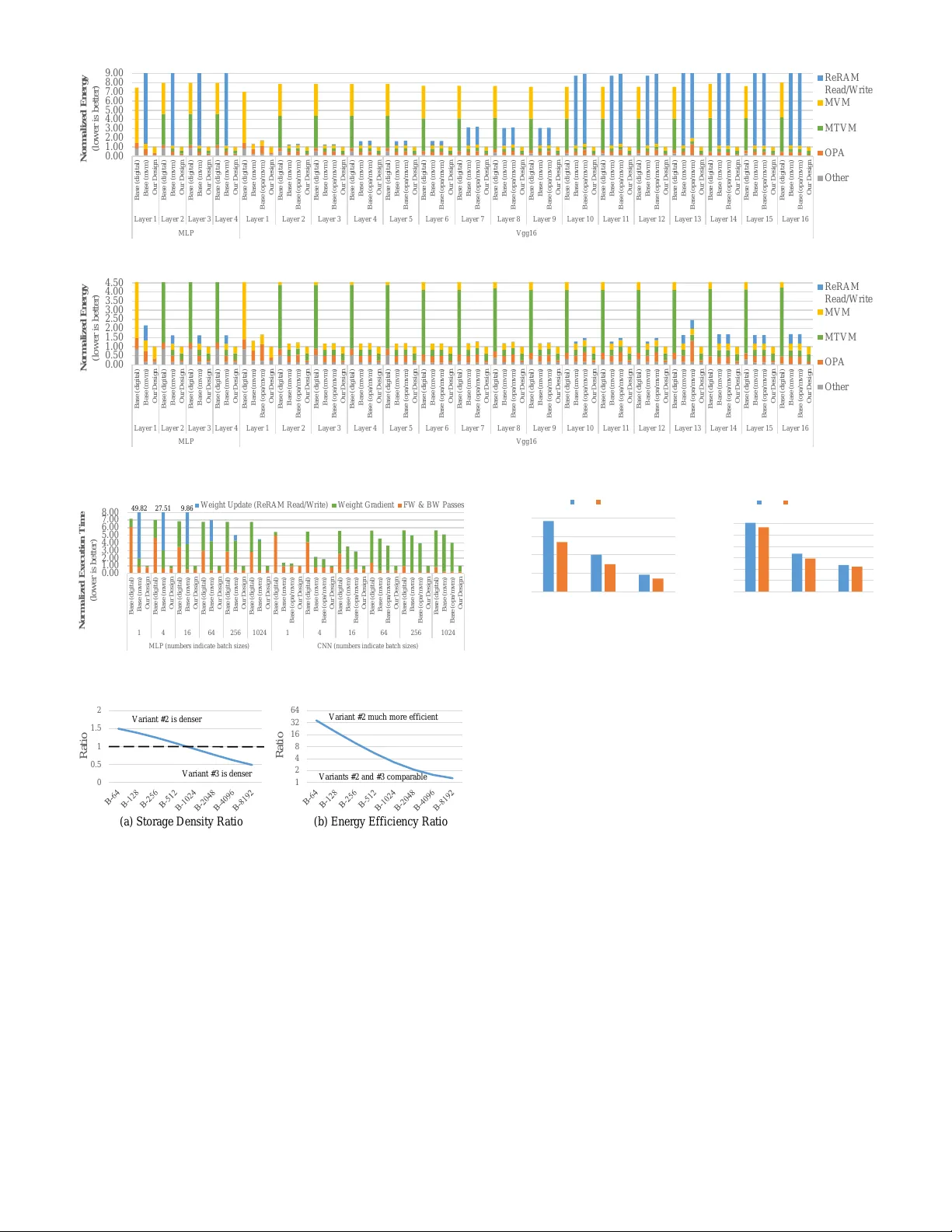
P ANTHER: A Progr ammab le Architecture f or Neur al Network T raining Har nessing Energy-efﬁcient ReRAM Aa yush Ankit, Izzat El Hajj, Sai Rahul Chalamalasetti, Sapan Agarwal, Matthe w Marinella, Mar tin F oltin, John P aul Strachan, Dejan Milojicic , Wen-mei Hwu, and Kaushik Ro y . Abstract —The wide adoption of deep neural networks has been accompanied by e ver-increasing energy and perf ormance demands due to the expensiv e nature of training them. Numerous special-purpose architectures have been proposed to acceler ate training: both digital and hybrid digital-analog using resistiv e RAM (ReRAM) crossbars. ReRAM-based accelerators ha ve demonstrated the effectiv eness of ReRAM crossbars at perf or ming matrix-v ector multiplication operations that are pre valent in tr aining. Howe ver , they still suffer from inefﬁciency due to the use of serial reads and writes for perf orming the weight gradient and update step . A fe w works hav e demonstrated the possibility of performing outer products in crossbars, which can be used to realiz e the weight gradient and update step without the use of serial reads and writes. Howe v er , these works have been limited to lo w precision operations which are not sufﬁcient f or typical training workloads. Moreov er , they ha ve been conﬁned to a limited set of training algorithms for fully-connected la yers only . T o address these limitations, we propose a bit-slicing technique f or enhancing the precision of ReRAM-based outer products, which is substantially different from bit-slicing f or matrix-vector multiplication only . We incorporate this technique into a crossbar architecture with three variants catered to diff erent training algorithms. T o e valuate our design on diff erent types of lay ers in neural networks (fully-connected, conv olutional, etc.) and training algorithms, we de velop P ANTHER, an ISA-programmable tr aining accelerator with compiler suppor t. Our design can also be integrated into other acceler ators in the literature to enhance their efﬁciency . Our ev aluation shows that P ANTHER achieves up to 8 . 02 × , 54 . 21 × , and 103 × energy reductions as well as 7 . 16 × , 4 . 02 × , and 16 × ex ecution time reductions compared to digital accelerators, ReRAM-based acceler ators, and GPUs, respectiv ely . F 1 I N T R O D U C T I O N Deep Neural Networks (DNNs) have seen wide adoption due to their success in many domains such as image pr ocess- ing, speech recognition, and natural language processing. However , DNN training requir es substantial amount of computation and energy which has led to the emergence of numerous special-purpose accelerators [1]. These accel- erators have been built using various circuit technologies, including digital CMOS logic [2], [3] as well as hybrid digital-analog logic based on ReRAM crossbars [4], [5]. ReRAM crossbars ar e circuits composed of non-volatile elements that can perform Matrix-V ector Multiplication (MVM) in the analog domain with low latency and energy consumption. Since MVM operations dominate the perfor- mance of DNN inference and training, various inference [4], [5], [6] and training [7], [8] accelerators have been built using these cr ossbars. However , while infer ence algorithms do not modify matrices during execution, training algorithms modify them during the weight gradient and update step (weight gradient computation followed by the weight up- date). For this reason, training accelerators [7], [8] require frequent reads and write to crossbar cells to realize weight • A. Ankit, and K. Roy are with the Department of Electrical and Computer Engineering, Purdue University. • I. E. Hajj is with the Department of Computer Science, American Univer- sity of Beirut. • S. R. Chalamalasetti, M. Foltin, J. P . Strachan, and D. Milojicic are with the Hewlett Packard Labs. • S. Agarwal, and M. Marinella are with the Sandia National Labs. • W . Hwu is with the Department of Electrical and Computer Engineering, University of Illinois at Urbana-Champaign. Correspondance email: aankit@purdue.edu 1.0 10.0 100.0 1,000.0 10,000.0 MVM Matrix Read Matrix Write Energy ( nJ ) CMOS ReRam 10.4× 9.8× 100.0 1,000.0 10,000.0 100,000.0 MVM Matrix Read Matrix Write Latnecy ( ns ) CMOS ReRam 8.9× 8.7× 17.5× Fig. 1. Comparing CMOS and ReRAM Primitives gradient and update operations. These reads and writes to ReRAM crossbars are performed one row at a time (like a typical memory array), and are referr ed to as serial reads and writes in this paper . Figure 1 compares the energy and latency of CMOS and ReRAM technologies for various primitive operations. As shown, MVM consumes ' 10 . 4 × less energy and has ' 8 . 9 × lower latency with ReRAM over CMOS (at same area) for a 32 nm technology node. However , reading and writing the entir e matrix consumes much higher energy and latency with ReRAM. Particularly , ReRAM writing energy and latency are an order of magnitude higher due to the cost of the program-verify approach which requir es tens of pulses [9]. Therefore, the use of serial reads and writes during training takes away the overall beneﬁts gained from using ReRAM for acceleration. T o overcome this issue, recent demonstrations [10], [11] have shown that Outer Product Accumulate (OP A) opera- tions can be performed in crossbars to realize the weight gradient and update operations without the use of serial reads and writes. The OP A operation is performed by 2 applying two input vectors at the rows and the columns of a crossbar simultaneously , to update each cell depend- ing on the inputs at the corresponding row and column. However , these demonstrations are limited to low-precision inputs/outputs (2-4 bits) and weights (2-5 bits) which is not sufﬁcient for the typical training workloads [12], [13]. Moreover , they are conﬁned to Stochastic Gradient Descent (SGD) with batch size of one for fully-connected layers only . T o address these limitations, we propose a bit-slicing technique for achieving higher precision OP A operations by slicing the bits of the output matrix weights across multiple crossbars. While bit-slicing has previously been done for MVM operations [4], bit-slicing matrices to also support OP A operations is substantially differ ent. For MVM, the rows and the crossbar cells are inputs and the columns are outputs, whereas for OP A, the rows and the columns are both inputs and the outputs are the crossbar cells themselves. Moreover , bit-slicing OP A presents additional constraints for the distribution of bits across the slices. First, weights are constant during MVM, but they change during OP A, which necessitates support for overﬂow within each slice and accounting for saturation. Second, MVM favors fewer bits per slice to reduce analog-to-digital Converter (ADC) precision requirements [4], but we show that OP A favors mor e bits per slice. Third, MVM favors homogeneous slicing of bits (equal number of bits per slice), but we show that OP A favors heterogeneous slicing. W e incorporate our proposed technique for enhancing OP A precision into a crossbar architectur e that performs both MVM and OP A operations at high precision. W e present three variants of the crossbar architecture that are catered to differ ent training algorithms: SGD, mini-batch SGD, and mini-batch SGD with large batches. Using this crossbar architectur e, we build P ANTHER, a Programmable Architectur e for Neural Network Training Harnessing Energy-ef ﬁcient ReRAM. W e use P ANTHER to evaluate our design on differ ent layer types (fully-connected, convolu- tional, etc.) and training algorithms. Our design can also be integrated into existing training accelerators in the literature to enhance their efﬁciency . Our evaluation shows that P AN- THER achieves up to 8 . 02 × , 54 . 21 × , and 2 , 358 × energy reductions as well as 7 . 16 × , 4 . 02 × , and 119 × execution time reductions compared to digital accelerators, ReRAM-based accelerators, and GPUs, respectively . W e make the following contributions: • A bit-slicing technique for implementing high- precision OP A operations using ReRAM crossbars (Section 3) • A cr ossbar-based ar chitecture, that embodies this bit- slicing technique, with three variants for differ ent training algorithms (Section 4) • An ISA-programmable accelerator with compiler support to evaluate differ ent types of layers in neural networks and training algorithms (Section 5) W e begin with a background on the use of ReRAM crossbars for DNN training (Section 2). 2 B AC K G R O U N D 2.1 Deep Neural Netw ork T raining T ypical DNN training comprises of iterative updates to a model’s weights in order to optimize the loss based on an W X H 𝐻 = 𝑊 . 𝑋 x 1 x 2 x 3 x 4 h 1 h 2 h 3 h 4 w ij 1 (a) FC Layer Forw ard Pass δW δX δH δx 1 δx 2 δx 3 δx 4 δh 1 δh 2 δh 3 δh 4 w ij δX = 𝑊 𝑇 . 𝑑𝐻 δW = δ 𝐻 𝑇 . 𝑋 2 3 (b) FC Layer Backw ard Pass H h1 (δh 1 ) δH 2 w 11 w 12 w 13 w 14 w 21 w 22 w 23 w 24 w 31 w 32 w 33 w 34 w 41 w 42 w 43 w 44 (δx 1 ) x 1 (δx 2 ) x 2 (δx 3 ) x 3 (δx 4 ) x 4 X 1 ( δX ) h2 (δh 2 ) h3 (δh 3 ) h4 (δh 4 ) (c) MVM and M T VM in Crossba rs X δH 3 x 2 x 3 x 4 δh 1 δh 2 δh 3 δh 4 w 11 w 12 w 13 w 14 w 21 w 22 w 23 w 24 w 31 w 32 w 33 w 34 w 41 w 42 w 43 w 44 (d) OP A in Crossba rs x 1 Fig. 2. FC Lay er Matrix Operations in Crossbars objective function. Equations 1–4 show the steps involved in DNN training based on the Stochastic Gradient Descent (SGD) algorithm [14]. Equation 1 constitutes the forward pass which processes an input example to compute the activations at each layer . Equation 2 computes the output error and its gradient based on a loss function using the activations of the ﬁnal layer . Equations 3 constitutes the backward pass which propagates the output error to com- pute the errors at each layer . Finally , equation 4 computes the weight updates to minimize the error . H (l+1) = W (l) X (l) , X (l+1) = σ ( H (l+1) ) (1) E = Loss ( X (L) , y ) , δ H (L) = ∇ E  σ 0 ( X (L) ) (2) δ H (l) = [( W l ) T δ H (l+1) ]  σ 0 ( X (l) ) (3) ∂ E ∂ W l ( or δ W l ) = X (l) ( δ H (l+1) ) T , W l = W l − η ∗ ∂ E ∂ W l (4) 2.2 Using Cr ossbars for T raining The most computationally intensive DNN layers that are typical targets for acceleration are the fully-connected layers and the convolutional layers. W e use fully-connected layers as an example to show how ReRAM crossbars can be used to accelerate DNN training workloads. 2.2.1 Ov er view of Fully Connected (FC) Layers Figures 2(a) and (b) illustrate the operations involved during training in a FC layer . The training involves three types of matrix operations: ¶ activation , · layer gradients , and ¸ weight gradients . Activation corresponds to an MVM opera- tion with the weight matrix ( W ), as shown in Equation 1. Layer gradients correspond to an MVM operation with the transpose of the weight matrix (hereon denoted as M T VM), as shown in Equation 3. W eight gradients correspond to an outer product operation, the result of which is accumulated to the weight matrix based on the learning rate ( η ), as shown in Equation 4. Ther efore weight gradients and updates together can be viewed as an Outer Product Accumulate (OP A) operation on the weight matrix. 3 R OFF R ON W ij =0 - Δ W ij + Δ W ij W ij =0 R OFF R ON + Δ W ij (e) Po sitiv e and Negativ e Gradien ts 𝑻𝑺 𝟏𝟓 : Sli ce - 7 Sli ce - 6 Sli ce - 5 Sli ce - 4 Sli ce - 3 Sli ce - 2 Sli ce - 1 Sli ce - 0 Ma tri x weight ( cross point ) sta te across slice s (cr oss bars) 0001 00 0010 00 0001 00 0100 00 101 1 00 1010 00 1000 00 1111 00 1010 00 0 1 1 0 00 0101 00 00 1 1 1 0 00 1 1 0 0 00 11 1 0 1 1 11 𝑾 𝒏𝒆𝒘 = 𝑾 𝒐𝒍𝒅 + 𝚫 𝑾 ( 𝜟 𝑾 = 𝒂 ∗ 𝒃 ) 1 1 1 0 1 1 0 0 𝑾 𝒐𝒍𝒅 + ( 𝒂 ≪ 𝟎 ) ∗ 𝒃 0 𝑾 𝒑𝒓 𝒆𝒗 + ( 𝒂 ≪ 𝟏𝟓 ) ∗ 𝒃 𝟏𝟓 𝑾 𝒑𝒓 𝒆𝒗 + ( 𝒂 ≪ 𝒏 ) ∗ 𝒃𝒏 𝑻𝑺 𝟎 : 𝑻𝑺 𝒏 : (d ) 1 6 - bi t OP A Ex ecutio n W 11 W 12 W 13 W 14 W 21 W 22 W 23 W 24 W 31 W 32 W 33 W 34 W 41 W 42 W 43 W 44 10010…0 101 10…1 1 1 1 10…1 001 10…0 00 01 10 11 0 1 1 0 1 - bit DAC 2 - bit DAC (b ) S tream in g Row In pu t Bits n - bit Inpu t 1 1 00 01 10 11 0001…101 1 2 - bit DAC 1 - bit DAC 101 10…1 n - bit Inpu t 1 n - bit Inpu t 2 (c) Slicin g Col um n In pu t Bits W ij slice N W ij slice N - 1 W ij slice 1 W ij slice 0 W 11 W 12 W 13 W 14 W 21 W 22 W 23 W 24 W 31 W 32 W 33 W 34 W 41 W 42 W 43 W 44 00 01 10 11 00 01 10 11 2 - bi t D A C (enco de i n ti m e) 2 - bi tD A C (enco de i n a m pl i tude) (a) 2 - bi t OP A Co lumn DA C Reso lution ( p ) Ma x Bi ts per W ei gh t Sli ce T ot al Bi ts fo r 32 - bit W ei gh t 2 5 62 3 6 47 4 6 41 5 7 35 (f) Bit Usage fo r Dif ferent Resolu tio ns cro ssb ar N cro ssb ar N - 1 cro ssb ar 1 cro ssb ar 0 New W ei ght Old W ei gh t No nega tive upda te po ssibl e T ime - Steps (TS) Fig. 3. Bit Slicing OP A to Enhance its Precision 2.2.2 Activ ation and La yer Gradients in Crossbars Figure 2(c) shows how a ReRAM crossbar can be used to compute activation and layer gradients. The weights of the matrix ( W ) are stored in the crossbar cells as the conductance state [15]. The MVM operation is realized by applying the input vector ( X ) as voltages on the rows of crossbar . Subsequently , the output vector ( H ) is obtained as currents from the columns. The M T VM operation is realized by applying the input vector ( δ H ) as voltages on the columns of the crossbar . Subsequently , the output vector ( δ X ) is obtained as currents from the rows. Both MVM and M T VM operations execute O ( n 2 ) multiply-and-accumulate operations in one computational step in the analog domain ( n is the crossbar size). Therefore, ReRAM cr ossbars can be leveraged to design highly ef ﬁcient primitives for activation and layer gradient computations. For this reason, they have been extensively considered for DNN inference [4], [5], [16] and training [7], [8] accelerators. 2.2.3 W eight Gradients and Updates in Crossbars Figure 2(d) shows how a ReRAM crossbar can be used to compute weight gradients. The OP A operation can be realized by applying the inputs ( X and δ H ) as voltages on the crossbar ’s rows and columns, respectively . The change ( w i j − w i j ) in the value stored at a cross-point ( i, j ) is equal to the product of the voltage on row i and column j (details in Section 3). Therefore, the outer product operation in the crossbar is naturally fused with the weight matrix accumulate operation. The OP A operation executes O ( n 2 ) multiply-and- accumulate operations in one computational step in the analog domain. It avoids serial reads and writes to ReRAM crossbar cells, which is important because reads and writes have orders of magnitude higher cost (energy and latency) than in-crossbar computations (MVM, M T VM, OP A). There- fore, ReRAM crossbars can be leveraged to design highly efﬁcient primitives for weight gradient computation and weight update. The aforementioned technique has been demonstrated with low-precision inputs/outputs (2-4 bits) and weights (2-5 bits) on the SGD training algorithm for FC layers only [10], [11]. In this paper , we enhance the technique with architectur e support to increase its precision and cater to a multiple training algorithms and differ ent layer types. 3 E N H A N C I N G R E R A M - B A S E D O P A P R E C I S I O N DNN workloads r equire 16 to 32 bits of precision for training [12], [13]. However , input digital-to-analog convert- ers (DACs), crossbar cells, and output ADCs cannot sup- port such levels of precision due to technology limitations and/or energy considerations. For this reason, accelerators that use ReRAM crossbars for MVM/M T VM operations typically achieve the requir ed precision with bit-slicing [4], where matrix bits ar e sliced across the cells of multiple cross- bars, input bits are streamed at the crossbar rows/columns, and shift-and-add logic is used to combine the output bits at each column/row across crossbars (slices). Bit-slicing matrices to also support OP A operations is differ ent because both the rows and columns are simulta- neously applied as inputs and the outputs are the crossbar cells themselves. Moreover , bit-slicing for OP A operations presents additional constraints for the choice of bit distri- bution across slices. This section describes our technique for bit-slicing the OP A operation (Section 3.1), and discusses the constraints it adds to the choice of bit distribution and how we address them (Sections 3.2 to 3.4). 4 3.1 Bit Slicing the OP A Operation Figure 3(a) illustrates how the OP A operation is performed when 2-bit inputs are applied at the rows and the columns. The digital row input is encoded in the time-domain us- ing pulse-width modulation. The digital column input is encoded in the amplitude-domain using pulse-amplitude modulation. Both pulse-width and pulse-amplitude modu- lations can be implemented using DACs. The weight change in a cell depends on the duration and the amplitude of the pulses applied on the corresponding row and column respectively , ther eby realizing an analog OP A operation [10], [11]. T o perform an OP A operation with 16-bit inputs, naively increasing the DAC resolution is infeasible because DAC power consumption grows rapidly with resolution ( N ) as: P DAC = β (2 N / N + 1) V 2 f clk [17] (5) Instead, we propose an architectural scheme to realize a 16-bit OP A operation by bit-streaming the row input bits, bit-slicing the column input bits, and bit-slicing the matrix weights across multiple crossbars. Figure 3(b) illustrates how we stream row input bits, m bits at a time over 16 /m cycles. Meanwhile column input bits are left-shifted by m -bits every cycle. Since the number of cycles decrease linearly with m while the cycle duration increases exponentially with m due to pulse-width modulation of row input, we choose m = 1 to minimize total latency . Using m = 1 also means that the row DACs are just inverters, thereby having low power consumption. Figure 3(c) shows how we slice column input bits across crossbars. Only one weight W ij is shown for clarity . In each cycle, the left-shifted column input is divided into chunks of p bits ( p = 2 in this example) and each chunk is applied to the corresponding crossbar . Figure 3(d) illustrates the steps for a 16-bit × 16-bit OP A operation at one crosspoint in the crossbar , resulting in a 32-bit output value for each matrix weight. It puts together the bit-streaming of the row input vector b and bit-slicing of the column input vector a with p = 4 . Each dot represents a partial product ( a n .b n ) , and the color corresponds to a speciﬁc weight slice (crossbar). Thus, the net accumulation to a slice is the result of all partial products of the speciﬁc color . The updated weight after a time step T n can be expressed as: W updated = W old + n X n =0 ( a << n ) ∗ b n (6) Crossbars store data in unsigned form. T o enable positive and negative weight updates ( δ W ), we repr esent inputs in the signed magnitude r epresentation. T o enable a symmetric repr esentation of positive and negative weight updates, we bias each device such that, a zero weight ( W ij ) is repre- sented by the memory state ( R ON + R OFF ) / 2 , as shown in Figure 3(e). Hence, the signed magnitude computation and biased data representation enable both positive and negative updates to weights. This is important as both polarities of updates are equally important in DNN training. Such a biased-repr esentation can be implemented by adding an extra column per crossbar ( 128 rows, 128 columns) with minimal area/ener gy cost [18]. 3.2 Bits to Handle Overﬂow For MVM/M T VM, the matrix weights are inputs to the operation and they do not change. In contrast, for OP A, the matrix weights are accumulated with the values resulting from the outer pr oduct. As a result, the weight slice stor ed in a crossbar cell may overﬂow , either from multiple accumu- lations within one OP A or over multiple OP As. W e handle this overﬂow by provisioning weight slices with additional bits to store the carry (shaded bits shown in Figure 3(d)). Propagating carry bits to other slices would r equire serial reads and writes which incur high overhead. For this reason, we do not propagate the carry bits immediately . Instead, they are kept in the slice and participate in future MVM/M T VM and OP A operations on the crossbar . The carry bits cannot be kept in the weight slice in- deﬁnitely because eventually the weight slice may get saturated i.e. crossbar cell at maximum/minimum state for positive/negative update. Saturation is detrimental for trainability (desirable loss r eduction during training) because it freezes training progress due to the absence of weight change. For this reason, we employ a periodic Carry Resolu- tion Step (CRS) which executes infrequently to perform carry propagation using serial reads and writes. W e evaluate the impact of the number of bits provisioned per slice and the CRS frequency on saturation and accuracy in Section 7.1. 3.3 Number of Slices vs. Bits P er Slice When slicing matrix bits across multiple crossbars, there is a tradeoff between the number of slices and the number of bits per cell in each slice. MVM operations favor using more slices and fewer bits per slice. The reason is that energy increases linearly with the number of crossbars, and non-linearly with the precision of a crossbar due to the increase in ADC precision requir ed to support it. Therefore, using more slices with fewer bits each is better for energy consumption. In contrast, OP A favors having fewer slices with more bits per slice. The reason is that OP A introduces carry bits to each slice and having more slices with fewer bits each increases the overhead from the carry bits. For example, Figure 3(f) shows that with 2 bits per slice, 62 total bits are requir ed to repr esent the 32-bit weight while capturing the carry bits adequately . T o strike a balance, we choose p = 4 , since p > 4 requir es a device precision that exceeds ReRAM technology limits [15]. A 4-bit DAC resolution is feasible because DAC power does not increase rapidly at low resolution (Equa- tion 5). By choosing p = 4 , our MVM/M T VM operations consume more energy than other ReRAM-based accelera- tors. However , our more energy efﬁcient OP A operations compensate because they avoid the need for expensive serial reads and writes. 3.4 Heter ogeneous Weight Slicing MVM operations favor homogeneous bit-slicing. Increasing the precision of one slice while decreasing the precision of another is always an unfavorable tradeoff because energy increases nonlinearly with the pr ecision of a crossbar . In con- trast, for OP A operations where crossbar values change, pr o- visioning more bits for slices that experience more weight 5 T ra inin g step s T ra inin g step s A v erage o f Norm ali zed Gradein ts ( Δ W/W ) Ab so lu te weig h t r an g e Fig. 4. Weight Gr adients across T raining Steps updates helps reduce the frequency of saturation, thereby ensuring trainability while keeping the frequency of CRS low . Heterogeneous weight slicing provisions more bits for matrix slices that change more frequently . The frequency of change is impacted by two factors: OP A asymmetry and the small weight gradient range in DNNs. OP A asymmetry is illustrated in Figure 3(d) where the central slices receive more partial products (dots) than the edge slices, which motivates increasing precision for the central slices. Small weight gradient range is shown in Figure 4 where weight updates form a very small fraction ( 2% − 5% ) of the overall weight range for > = 95% of training steps, which moti- vates increasing precision of the lower slices. W e evaluate the impact of heterogeneous weight slicing on energy and accuracy in Section 7.2. 4 M AT R I X C O M P U TA T I O N U N I T ( M C U ) The techniques described in Section 3 ar e incorporated into a Matrix Computation Unit (MCU) for DNN training accelerators. This section ﬁrst describes the MCU’s orga- nization (Section 4.1). It then describes the three variants of the MCU optimized for SGD (Section 4.2), mini-batch SGD (Section 4.3), and mini-batch SGD with large batches (Section 4.4). 4.1 MCU Organization Figure 5 illustrates the or ganization of the MCU. Performing an MVM operation with the MCU is illustrated by the red arrow . Digital inputs stored in the XBarIn registers are fed to the crossbar rows through the Input Driver . The output currents from the crossbar columns are then then converted to digital values using ADC and stored in the XBarOut registers. Performing a M T VM operation in the MCU is illustrated by the purple arrow in Figure 5. The key difference com- pared to the MVM operation is the addition of multiplexers to supply inputs to crossbar columns instead of rows and to read outputs from crossbar rows instead of columns. MVM and M T VM operations require 16 to 32 bits of precision for training [2]. W e use 16-bit ﬁxed-point rep- resentation for input/output data and 32-bit ﬁxed-point repr esentation for weight data which ensures sufﬁcient pre- cision [12]. Performing an OP A operation in the MCU is illustrated by the blue arrow in Figure 5. Digital inputs stored in the XBarIn registers are fed to the crossbar rows through the Input Driver . Digital inputs stored in the XBarOut registers are fed to the crossbar columns through the Input Driver . The Xba rIn Re gisters ADC Pipel ined MCU In p u t D ri v er (DA C) In p u t D ri v er (DA C) Row D eco d er f rom Instructio n Decod e Cro ss b ar Arr ay Xba rOu t Re gisters MVM M T VM OP+U pd ate Rea d/W rite to VFU + V dd - V dd Gn d Sel ect L o g i c Sig n LSB A D C: A n al o g t o D i g i t al Co n v ert er D A C: D i g i t al t o A n al o g Co n v ert er Fig. 5. Matrix Computation Unit T ABLE 1 Dataﬂow f or SGD T ime Step MCU0 (Layer1) MCU1 (Layer2) MCU2 (Layer3) 0 MVM (a0) (a1) 1 MVM (a1) (a2) 2 MVM (a2) (a3) 3 M T VM ( δ h3) ( δ h2) 4 M T VM ( δ h2), ( δ h1) OP (a2 , δ h3) ( ∇ W3) 5 OP (a0, δ h1) ( ∇ W1) OP (a1, δ h2) ( ∇ W2) effect of this operation is that the outer product of the input vectors is accumulated to the matrix stored in the crossbar . T o support positive and negative inputs, the input drivers in Figure 5 use the sign bit (MSB) to drive the crossbar rows and columns with positive or negative voltages. 4.2 V ariant #1 for SGD Acceleration SGD-based training performs example-wise gradient de- scent. First, an input example performs a forward pass (MVM) to generate activations - H l . Next, the error com- puted with respect to the activation of the output layer is back propagated (M T VM) to compute the layer gradients - δ X l . Finally , the activations and layer gradients are used to update (OP A) the weight matrix - W l , before the next input example is supplied. T able 1 illustrates the logical execution of matrix opera- tions in three MCUs for a three-layer DNN with an input example a 0 . Each time step shows the operations executed on each MCU and their inputs/outputs. For example, at time step 0 , MCU0 performs an MVM operation on input a 0 to compute the output a 1 . The illustration assumes that each layer maps on one MCU and does not show the interleaved nonlinear operations for clarity . For a layer size larger than one MCU capacity ( 128 × 128 matrix), the layer is partitioned across multiple MCUs (see Section 5.3). V ariant #1 of the MCU uses a single crossbar to perform all three matrix operations: MVM, M T VM, and OP A. This variant is suitable for SGD because, as shown in T able 1, the three matrix operations are data dependent and will never execute concurrently . However , this variant creates struc- tural hazar ds for mini-batch SGD as described in Section 4.3. 4.3 V ariant #2 for Mini-Batc h SGD Acceleration Mini-batch SGD performs batch-wise gradient descent. Like SGD, each input performs MVM, M T VM, and OP A to compute activations, layer gradients, and weight gradi- ents/updates, respectively . However , the weight update is 6 T ABLE 2 Dataﬂow f or Mini-Batch SGD T ime Step MCU0 (Layer1) MCU1 (Layer2) MCU2 (Layer3) 0 MVM (a 0 0) (a 0 1) 1 MVM (a 1 0) (a 1 1) MVM (a 0 1) (a 0 2) 2 MVM (a 2 0) (a 2 1) MVM (a 1 1) (a 1 2) MVM (a 0 2) (a 0 3) 3 MVM (a 3 0) (a 3 1) MVM (a 2 1) (a 2 2) MVM (a 1 2) (a 1 3) M T VM ( δ h 0 3) ( δ h 0 2) 4 MVM (a 4 0) (a 4 1) MVM (a 3 1) (a 3 2) MVM (a 2 2) (a 2 3) M T VM ( δ h 0 2), ( δ h 0 1) M T VM ( δ h 1 3) ( δ h 1 2) 5 MVM (a 4 1) (a 4 2) MVM (a 3 2) (a 3 3) M T VM ( δ h 1 2), ( δ h 1 1) M T VM ( δ h 2 3) ( δ h 2 2) 6 MVM (a 4 2) (a 4 3) M T VM ( δ h 2 2), ( δ h 2 1) M T VM ( δ h 3 3) ( δ h 3 2) 7 M T VM ( δ h 3 2), ( δ h 3 1) M T VM ( δ h 4 3) ( δ h 4 2) 8 M T VM ( δ h 4 2), ( δ h 4 1) 9-12 OP (a n 0, δ h n 1) ( ∇ W n 1) OP (a n 1, δ h n 2) ( ∇ W n 2) OP (a n 2, δ h n 3) ( ∇ W n 3) Iterate for n=1 to 4 only reﬂected at the end of a batch to be used by the inputs of the next batch. T able 2 illustrates the logical execution of matrix opera- tions for a batch of ﬁve inputs, where a n m refers to the m th activation of n th input. MVM operations can be executed for multiple input examples concurr ently in a pipelined fashion ( MVM (a 1 0) (a 1 1), MVM (a 0 1) (a 0 2) in T able 2). Additionally , the MVM and M T VM operations for different inputs in the batch can also execute in parallel during the same timestep, provided that there is no structural hazard on the MCU. The desire to eliminate such structural hazards motivates V ariant #2. V ariant #2 of the MCU eliminates structural hazards in mini-batch SGD by storing two copies of the matrix on differ ent crossbars, enabling the MCU to perform MVM and M T VM in parallel. This replication improves the energy- delay product for a batch. W ith < 2 × increase in area, we improve the batch latency by O ( L ) , where L is the number of layers. The ISA instruction for performing MVM/M T VM (Section 5.2) is designed to enable the compiler (Section 5.3) to schedule these two operations in parallel on the same MCU. The OP A operations are executed at the end of the mini- batch (steps 9-12 in T able 2) to reﬂect the weight updates for the entire batch. These OP A operations require that the vectors involved are saved until then. V ariant #2 saves these vectors in shar ed memory . However , if the batches ar e large, this approach puts too much stress on the shared memory which motivates V aiant #3 (Section 4.4). 4.4 V ariant #3 for Mini-Batc h SGD with Large Batches For mini-batch SGD with very large batch sizes, saving the vectors in shared memory requires large shared memory size which degrades storage density . V ariant #3 alleviates the pressur e shared memory size by maintaining three copies of each crossbar . The ﬁrst two copies enable perform- ing MVM and M T VM in parallel, similar to V ariant #2. The third copy is used to perform the OP A operation eagerly , as soon as its vector operands are available, without changing the matrices being used by the MVM and M T VM operations. Performing OP A eagerly avoids saving vectors until the end, r educing the pressure on the shared memory . However , using a third crossbar for OP A requires serial reads and writes to commit the weight updates to the ﬁrst and the D E C O D E Re g i s t e r F i l e MU FU FU FU VF U Dat a wr i t eb ack Deco d ed i n st r u ct i o n EX EC U TE X bar In Re gi s t e rs X bar O ut Re gi s t e rs M CU X bar In Re gi s t e rs X bar O ut Re gi s t e rs M CU T o/ F r om S ha r e d M e m or y F E T C H Core 1 S ha re d M e m ory Core 2 Core N -1 Core N Ne t wo r k - On -Chi p Core 1 S ha re d M e m ory Core 2 Core N -1 Core N (a ) (b ) Fig. 6. Architecture Overview second crossbars for MVM and M T VM in the next batch. Section 7.6 discusses the impact of these design choices. 5 P R O G R A M M A B L E A C C E L E R ATO R The MCU described in Section 4 can be integrated with prior ReRAM-based training accelerators [7], [8] to improve their efﬁciency . W e develop a programmable training accelerator named P ANTHER to evaluate our design by extending the PUMA ReRAM-based inference accelerator [6]. This sec- tion describes P ANTHER’s organization (Section 5.1), ISA considerations (Section 5.2), compiler support (Section 5.3), and an example of how to implement convolutional layers (Section 5.4). 5.1 Accelerator Organization P ANTHER is a spatial architectur e organized in three tiers: nodes, tiles, and cores. A node consists of multiple tiles connected via an on-chip network, and a tile consists of multiple cores connected to a shared memory , as illustrated in Figure 6(b). A core consists of multiple MCUs for ex- ecuting matrix operations, a digital CMOS-based vector functional unit (VFU) for executing arithmetic operations and non-linear functions, a register ﬁle, and a load/store memory unit. A core also features an instruction execution pipeline making the accelerator ISA-programmable. T o sup- port DNNs whose model storage exceeds a node’s total MCU capacity , multiple nodes can be connected via an interconnect. This organization is similar to PUMA ’s [6] and is not a contribution of this paper . The key distinction from PUMA is the MCU which supports M T VM and OP A opera- tions, not just MVM operations, as described in Section 4. 5.2 ISA Considerations The PUMA [6] ISA includes mvm instructions executed by crossbars, arithmetic/logic/nonlinear instructions executed by the VFU, load/store instructions to access shared mem- ory , send/receive instructions to communicate with other tiles, and control ﬂow instructions. W e extend the PUMA ISA to also include a mcu instruction for executing all three matrix operations (MVM, M T VM, OP A) on the MCU. The mcu instruction takes six 3-bit masks, where each mask corresponds to one of the MCUs on the core (up to six). The three bits in the mask correspond to the three sup- ported matrix operations (MVM, M T VM, OP A). If multiple bits are set, then the instruction executes the operations concurrently . For example, if mask 0 is set to ’110’ and mask 1 is set to ’011’, then MCU 0 will execute MVM and 7 M T VM simultaneously and MCU 1 will execute M T VM and OP A simultaneously . Hence, the incorporation of all three operations into a single instruction is important for being able to execute them concurrently . The mcu instruction does not take source and destination operands since these are implied to by XBarIn and XBarOut . The semantic of the OP A operation is that it takes effect at the end of the execution when a special halt instruction is invoked. This semantic allows the same code to work for any of the three MCU variants, making the choice of variant a microar chitectural consideration and the ISA agnostic to it. The implementation of the OP A semantic on each of the variants is as follows. Consider the case when all three bits of an MCU’s mask are set. In V ariant #1, MVM and M T VM will be serialized on the same crossbar , while the operands of OP A will be saved to shared memory then applied to that crossbar when halt is invoked. In V ariant #2, MVM and M T VM will be executed in parallel on the two crossbar copies, while the operands of OP A will be treated like in V ariant #1. In V ariant #3, MVM and M T VM will be executed in parallel on the ﬁrst two crossbar copies, while the operands of OP A will be applied to the third crossbar . The values of the third crossbar will then be copied to the ﬁrst two crossbars when halt is invoked. 5.3 Compiler Support The PUMA [6] compiler provides a high-level program- ming interface in C++ that allows programmers to express models in terms of generic matrix and vector operations. The compiler is implemented as a runtime library that builds a computational graph when the code is executed then compiles the graph to PUMA ISA code. The compiler partitions matrices into sub-matrices and maps these sub- matrices to differ ent MCUs, cores, and tiles. It then maps the operations in the graph to differ ent MCUs, cores, and tiles accordingly , inserting communication operations wher e necessary . The compiler then linearizes the graph, creating an instruction sequence for each core. It performs register allocation for each sequence, spilling registers to shared memory if necessary . Finally , it generates ISA code for each core, collectively comprising a kernel that runs on the accelerator . W e make the following extensions to the PUMA com- piler to support P ANTHER. W e extend the application pro- gramming interface (API) to allow programmers to deﬁne training matrices that support MVM, M T VM, and OP A operations. W e extend the intermediate representation to repr esent these matrices and include them in the partition- ing. W e also add an analysis and transformation pass for identifying MCU operations in the graph that can be fused and fusing them. This pass fuses MCU operations that do not have data dependences between them and that use differ ent MCUs on the same core or use the same MCU but are differ ent types of operations (MVM, M T VM, OP A). The fusing process is iterative because every time operations are fused, new dependences are introduced to the graph. Finally , we extend the code generator to support the new mcu ISA instruction. Note that since the model weights are not updated until the halt instruction at the end, the scope of a kernel is a w 111 w 2 1 1 w 3 1 1 w 4 1 1 w 1 1 2 w 212 w 312 w 412 w 121 w 221 w 321 w 421 w 122 w 222 w 322 w 422 1 x 11 x 12 x 21 x 22 h 111 h 21 1 h 31 1 h 41 1 x 12 x 13 x 22 x 23 h 1 12 h 212 h 312 h 412 T1 T2 T1 T2 Activa ti on: it erat ive MVM ( h k ) ij = 𝚺𝚺 ( w k ) mn x (i - 1 + m ) ( j - 1 + n ) m n (δ w k ) ij = 𝚺𝚺 ( δh k ) m n x (i - 1 + m ) ( j - 1 + n ) m n w 111 w 2 1 1 w 3 1 1 w 4 1 1 w 1 1 2 w 212 w 312 w 412 w 121 w 221 w 321 w 421 w 122 w 222 w 322 w 422 3 x 12 δh 111 δh 21 1 δh 31 1 δh 41 1 x 11 x 21 x 22 x 12 x 13 x 22 x 23 δh 1 12 δh 212 δh 312 δh 412 T1 T2 T1 T2 W eight gradie nts+update = it erati v e OP A 𝐻 = 𝑋 ∗ 𝑊 1 δ 𝑊 = 𝑋 ∗ δH 3 δX = 𝑊 ∗ δH 2 x 11 x 12 x 13 x 21 x 22 x 23 x 31 x 32 x 33 w 111 w 1 12 w 121 w 122 w 4ij w 1ij h 111 h 1 12 h 121 h 122 h 4ij h 1ij Input Co nvoluti on Operat ions W eight (a) (b ) (c) Outp ut Fig. 7. Conv olutional Lay er Matrix Operations in Crossbars single batch. Multiple batches are executed by invoking the kernel multiple times on differ ent input data. 5.4 Implementing Con volutional La yers ReRAM-based OP A has one-to-one correspondence to the weight gradient/update operation for FC layers (discussed in Section 2.2.3). By integrating this technique into a pro- grammable accelerator with compiler support, we enable the mapping of more complex layers on top of it such as convolutional layers. This section describes how convolu- tional layers can be implemented in our accelerator . Figure 7(a) shows a typical convolution layer and the associated operations during training. Like with FC layers, convolutional layers performs three types of matrix opera- tions: ¶ activation , · layer gradients , and ¸ weight gradients . Unlike FC layers, these operations are all convolutions ( ∗ ). 5.4.1 Activ ation and La yer Gradients Figure 7(b) shows how the convolution operation for acti- vation is implemented in the crossbar on top of the MVM primitive. This approach is similar to that used in existing accelerators [8]. The crossbar stores the convolution kernel in the form of linearized ﬁlters ( w k ), where each column corresponds to the weights associated with a speciﬁc output channel ( h k ). The convolution operation to compute acti- vations is implemented as an iterative MVM operation. An iteration is r epresented as a time step (T1/T2) in Figur e 7(b), and corresponds to a speciﬁc (i,j) pair . A block of input features ( X ) is applied to the crossbar ’s rows as convolution data in each iteration. In a similar manner , the convolution operation for layer gradients (not shown in the ﬁgure) is realized using iterative M T VM. The next layer ’s errors ( δ H ) are used as the convolution data and ﬂipped ﬁlters (vertically and horizontally) are used as the convolution kernel. 5.4.2 W eight Gradients Figure 7(c), shows our proposed technique for implement- ing the weight gradients convolution operation and weight 8 (a) (b) Fig. 8. Computational graph obtained using T ensorBoard for (a) example model (b) example model with P ANTHER OP A update in the crossbar on top of the OP A primitive. The weight gradient computation uses input features ( X ) as the convolution data and output feature’s errors ( δ H ) as the convolution kernel. Each iteration is repr esented as a time step (T1, T2) in Figure 7(c), and corresponds to a speciﬁc (i,j) pair . On every iteration, the output feature’s errors are applied on the columns, in a depth major order . Simultaneously , by applying the portion of input features that generate the corr esponding activations ( H ) on the rows, a partial convolution is obtained between X and δ H . Striding across the output feature’s errors and input features for n 2 time steps, where n is size of one output feature map, realizes the full convolution operation. Convolutions for differ ent output feature maps are performed in parallel across the crossbar ’s columns, using the same weight data layout as used in MVM and M T VM operations. T o the best of our knowledge, our work is the ﬁrst to formulate the weight gradients convolution operation in terms of outer products. 5.4.3 Comparison with Other Accelerators Existing ReRAM-based training accelerators such as PipeLayer [8] do not compute the weight gradient con- volutions using outer products, but rather , they compute them using MVM operations. This requires writing the convolution kernel ( δ H ) on the crossbar because the con- volution operation here uses non-stationary data ( δ H ) as the convolution kernel. The drawback of this approach is that the latency and energy consumption of the serial reads and writes is very high, taking away from the overall efﬁciency provided by ReRAM-based MVMs. 6 M E T H O D O L O G Y 6.1 Ar chitecture Simulator W e extend the PUMA [6] simulator to model the MCU unit and its associated instructions. The PUMA simulator is a detailed cycle-level architectur e simulator that runs applications compiled by the compiler , in order to evaluate the execution of benchmarks. The simulator models all the necessary events that occur in an execution cycle, including compute, memory and NoC transactions. T o estimate power and timing of the CMOS digital logic components, their R TL implementations are synthesized to the IBM 32nm SOI tech- nology library , and evaluated using the Synopsys Design T ABLE 3 Summary of platforms Parameter P ANTHER (1 node) Base digital (1 node) 2080-T i (1 card) SIMD lanes 108 M 108 M 4352 T echnology CMOS-ReRam (32 nm) CMOS (32 nm) CMOS (12 nm) Frequency 1 GHz 1 GHz 1.5 GHz Area 117 mm 2 578 mm 2 750 mm 2 TDP 105 W 839 W 250 W On-Chip Memory 72.4 MB 72.4 MB 29.5 MB T ABLE 4 Details of workloads Layer C M H/W R/S E/F Wt (MB) In (MB) Ops/B CNN-Vgg16 Conv1 3 64 32 3 32 0.003 0.006 368.640 Conv2 32 64 32 3 16 0.035 0.063 92.160 Conv3 64 128 16 3 16 0.141 0.031 209.455 Conv4 128 128 16 3 8 0.281 0.063 52.364 Conv5 128 256 8 3 8 0.563 0.016 62.270 Conv6 256 256 8 3 8 1.125 0.031 62.270 Conv7 256 256 8 3 4 1.125 0.031 15.568 Conv8 256 512 4 3 4 2.250 0.008 15.945 Conv9 512 512 4 3 4 4.500 0.016 15.945 Conv10 512 512 4 3 2 4.500 0.016 3.986 Conv11 512 512 2 3 2 4.500 0.004 3.997 Conv12 512 512 2 3 2 4.500 0.004 3.997 Conv13 512 512 2 3 1 4.500 0.004 0.999 Dense14 512 4096 - - - 4.000 0.001 1.000 Dense15 4096 4096 - - - 32.000 0.008 1.000 Dense16 4096 100 - - - 0.781 0.008 0.990 MLP-L4 Dense1 1024 256 - - - 0.500 0.002 0.996 Dense2 256 512 - - - 0.250 0.000 0.998 Dense3 512 512 - - - 0.500 0.001 0.998 Dense4 512 10 - - - 0.010 0.001 0.909 Compiler . For the on-chip SRAM memories, the power and timing estimates are obtained from Cacti 6.0. Subsequently , the power and timing of each component are incorporated in the cycle-level simulator in order to estimate the energy consumption. MCU Modelling. Since the MCU is built with analog components and cannot be synthesized with publicly avail- able libraries, we adopted the models from past works [4], [10] and ADC survey [19]. W e use the ReRam cr ossbar array and sample-and-hold circuit models in ISAAC [4]. W e used capacitive DACs and Successive Approximation Register (SAR) ADCs. The DAC area and power are estimated using the equations described in Saberi et al. [20]. The ADCs for differ ent pr ecisions namely 8-12 bits operating at a sampling frequency of 1 GH z are obtained from the ADC survey [19]. The ADC optimization technique in Newton [21] is incorpo- rated to avoid unnecessary ADC conversions. 6.2 Functional Sim ulator W e implement a functional simulator using T ensorFlow that models P ANTHER’s bit-sliced OP A technique. This simulator enables performing design space exploration (for accuracy) on large-scale DNNs to explore the bounds on heterogeneous weight slicing and CRS frequency for train- ability . Here, a layer ’s weights are repr esented as a multi- dimensional tensor of shape S × M × N , where S corre- sponds to a weight slice (discussed in Figure 3 (d)), and M and N correspond to the weight matrix’s dimensions re- spectively . Each weight slice can have a unique bit-pr ecision, to model heterogeneous conﬁgurations (Section 3.4). The weight values beyond the range permissible by the bit- precision are clipped to model a slice’s saturation. Subse- quently , the weight update operation in native T ensorFlow is modiﬁed to quantize and bit-slice the computed weight gradients and then update the previous copy of weights (al- ready quantized and bit-sliced). Figures 8 (a) and (b) show 9 0% 5% 1 0 % 1 5 % 2 0 % 2 5 % 0 2 0 , 0 0 0 4 0 , 0 0 0 6 0 , 0 0 0 8 0 , 0 0 0 0% 5% 1 0 % 1 5 % 2 0 % 2 5 % 0 2 0 , 0 0 0 4 0 , 0 0 0 6 0 , 0 0 0 8 0 , 0 0 0 0% 5% 1 0 % 1 5 % 2 0 % 2 5 % 0 2 0 , 0 0 0 4 0 , 0 0 0 6 0 , 0 0 0 8 0 , 0 0 0 0% 5% 1 0 % 1 5 % 2 0 % 2 5 % 0 2 0 , 0 0 0 4 0 , 0 0 0 6 0 , 0 0 0 8 0 , 0 0 0 0% 5% 1 0 % 1 5 % 2 0 % 2 5 % 0 2 0 , 0 0 0 4 0 , 0 0 0 6 0 , 0 0 0 8 0 , 0 0 0 0% 5% 1 0 % 1 5 % 2 0 % 2 5 % 0 2 0 , 0 0 0 4 0 , 0 0 0 6 0 , 0 0 0 8 0 , 0 0 0 0% 5% 1 0 % 1 5 % 2 0 % 2 5 % 0 2 0 , 0 0 0 4 0 , 0 0 0 6 0 , 0 0 0 8 0 , 0 0 0 0% 5% 1 0 % 1 5 % 2 0 % 2 5 % 0 2 0 , 0 0 0 4 0 , 0 0 0 6 0 , 0 0 0 8 0 , 0 0 0 3 b i t s 4 b i t s 5 b i t s 6 b i t s 0% 2 0 % 4 0 % 6 0 % 8 0 % 1 0 0 % 0 2 0 , 0 0 0 4 0 , 0 0 0 6 0 , 0 0 0 8 0 , 0 0 0 0% 2 0 % 4 0 % 6 0 % 8 0 % 1 0 0 % 0 2 0 , 0 0 0 4 0 , 0 0 0 6 0 , 0 0 0 8 0 , 0 0 0 0% 2 0 % 4 0 % 6 0 % 8 0 % 1 0 0 % 0 2 0 , 0 0 0 4 0 , 0 0 0 6 0 , 0 0 0 8 0 , 0 0 0 0% 2 0 % 4 0 % 6 0 % 8 0 % 1 0 0 % 0 2 0 , 0 0 0 4 0 , 0 0 0 6 0 , 0 0 0 8 0 , 0 0 0 % S a tu r a te d B its S li c e 0 % S a tu r a te d B its in S li c e 7 Ac c u r a c y Tr a i n i n g S t eps ( C R S e v e r y 6 4 e x a mp l e s) Tr a i n i n g S t eps ( C R S e v e r y 1 0 2 4 e x a mp l e s) Tr a i n i n g S t eps ( C R S e v e r y 4 0 9 6 e x a mp l e s) Tr a i n i n g S t eps ( C R S e v e r y 5 0 0 4 8 e x a mp l e s) Fig. 9. Impact of Slice Bits and CRS F requency on Accuracy the computational graphs for an example neural network model, and the example model augmented with P ANTHER OP A operation (shown in red) respectively . 6.3 Baselines W e evaluate P ANTHER against three weight-stationary ASIC baselines: Base digital , Base mvm , and Base opa/mvm , as well as one NVIDIA GPU platform - T uring R TX 2080-T i (2080-T i). Base digital uses a digital version of the MCU where weights are stored in an SRAM array within the core and matrix operations are performed with a digital VFU. Base digital is an adaptation of the digital baseline used in PUMA [6]. As shown in the PUMA work, this digital baseline is an optimistic estimate of the Google TPU [3]. It is optimistic because it uses weight-stationary MVM compu- tations similar to TPU, but assumes that the entire model is mapped using on-chip SRAM, ther eby avoiding the off-chip memory access costs in TPU. Therefor e, our comparisons with Base digital also serve as a lower-bound on P ANTHER’s improvements compared to TPU. The objective of compar- ing with Base digital is to demonstrate the beneﬁt of ReRAM- based computing over pure digital approaches. Base mvm uses ReRAM for MVM and M T VM, and a dig- ital VFU for OP A with serial reads/writes to the crossbar . Base opa/mvm is a replication of PipeLayer ’s [8] approach de- scribed in Section 5.4.3 and only applies to convolutional layers. It uses ReRAM for MVM and M T VM, and realizes OP A with ReRAM MVMs and serial reads/writes. The objective of comparing with Base mvm and Base opa/mvm is to demonstrate the beneﬁt of ReRAM-based OP A operations. Conﬁgurations. Base mvm and Base opa/mvm use 32-bit weights sliced across 16 slices with 2 bits each, which is optimal since crossbars only do MVM/M T VM. P ANTHER uses heterogeneous weight slicing with 32-bit weights rep- resented using 39 bits sliced across 8 slices distributed from MSB to LSB like so: 44466555 (unless otherwise speciﬁed). For this reason, P ANTHER consumes 17 . 5% higher energy for MVM/M T VM than Base mvm and Base opa/mvm due to higher ADC precision. W e also use a CRS frequency of 1024 steps (unless otherwise speciﬁed) which achieves similar accuracy as the software implementation. For all three ASIC baselines and P ANTHER, the hierarchical organization uses 138 tiles per node, with 8 cores per tile and 2 MCUs per core. T a- ble 3 summarizes the platforms. Note that both Base mvm and Base opa/mvm have same platform parameters as P ANTHER. 6.4 W orkloads W e use a 4-layered MLP model and Vgg-16 CNN model on SVHN and CIF AR-100 datasets, respectively . T able 4 details the layer details of the two models and their computational intensity (operations to byte ratio). The individual layers of the chosen MLP and CNN models span a wide range of computational intensity observed across the spectrum of neural network workloads. Thus, our workloads are well repr esentative of the large variety of layer types found in neural network models such as fully-connected, 2 D- convolution, point-wise convolution, etc. Similar to other ReRAM training accelerators [7], [8], we use ﬁxed-point arithmetic which has been shown to be successful for training large DNNs [13]. W e use the CIF AR- 100 dataset for CNN which is comparable to the ImageNet dataset in terms of training difﬁculty [22], [23]. However , ImageNet’s large image sizes make it difﬁcult to run the training ﬂow without actual hardware (CIF AR-100 requir es 2 days and ImageNet requir es 1 month on the simulator). 7 E VA L UAT I O N 7.1 Impact of Slice Bits and CRS Frequency on Accu- racy Figure 9 shows the impact of the number of bits used per slice (uniform weight slicing) and CRS frequency for the CNN benchmark. W e analyze the percentage of saturated cells per slice for a lower order and higher order slice, and their implications on CNN’s T op-5 training accuracy . Using 3 bits per slice shows signiﬁcantly higher per- centage of saturated cells for the lower order slice (Slice 0) than other conﬁgurations. Further , increasing the CRS frequency does not reduce the saturation fraction of Slice 0 at 3-bits. Consequently , the training accuracy with 3-bits slices remains very low throughout the training steps. 10 0 . 0 0 0 .2 0 0 . 4 0 0 . 6 0 0 .8 0 1 . 0 0 2 0 . 0 2 5 . 0 3 0 . 0 3 5 . 0 4 0 . 0 4 5 . 0 5 0 . 0 5 5 . 0 6 0 . 0 V a l i d a t i o n A c c u r a c y Energ y ( nJ ) 3 3 3 3 3 3 3 3 ( 2 4 ) 4 4 4 4 4 4 4 4 ( 3 2 ) 5 5 5 5 5 5 5 5 ( 4 0 ) 6 6 6 6 6 6 6 6 ( 4 8 ) 4 4 4 4 5 5 5 5 ( 3 6 ) 3 3 3 3 6 6 6 6 ( 3 6 ) 3 3 4 4 6 6 5 5 ( 3 6 ) 4 4 4 4 6 6 5 5 ( 3 8 ) 4 4 4 6 6 5 5 5 ( 3 9 ) 4 4 5 5 5 5 6 6 ( 4 0 ) 4 4 5 5 6 6 5 5 ( 4 0 ) 4 4 4 4 6 6 6 6 ( 4 0 ) 4 4 4 6 6 6 5 5 ( 4 1 ) 5 5 5 5 6 6 5 5 ( 4 2 ) 5 5 5 5 6 6 6 6 ( 4 4 ) 5 5 6 6 6 6 5 5 ( 4 4 ) H e t e r o g e n e o u s: H o mo g e n e o u s: Fig. 10. Heterogeneous Weight-Slicing Using 4 bits per slice performs well at high CRS fre- quency (CRS every 64 steps), but does not scale well at lower CRS frequencies. A high CRS frequency is undesirable due to the high cost of serial reads and writes incurred during carry propagation between discrete slices. Slices with 5-bits and 6-bits are robust to repeated weight updates as they exhibit lower saturation for both lower order and higher order slices even at low CRS frequencies (every 1024 or 4096 steps). Note that the cost of a CRS operation at low frequency (every 1024 steps) has negligible impact on overall energy and performance ( ≤ 4 . 8% ). Figure 9 also motivates heterogeneous weight slicing because it shows that the higher order slice has signiﬁcantly lower saturation in general than the lower order slice. 7.2 Impact of Heter ogeneous Weight Slicing Figure 10 shows the accuracy and energy of sixteen slic- ing conﬁgurations. Generally speaking, increasing the total number of bits improves accuracy by reducing saturation, but it also increases energy because it requir es higher pre- cision ADCs for MVM and M T VM. The graph shows that heterogeneous weight slicing enables favourable accuracy- energy tradeoffs, enabling lower energy at comparable accu- racy or better accuracy at comparable energy . Provisioning ≥ 4 bits for the four higher order slices ( 4 − 7 ) and ≥ 5 bits for the four lower order slices ( 0 − 3 ) ensures desirable accuracy . Any conﬁguration using 3 bit slices (irrespective of total bits) leads to signiﬁcant accuracy degradation. Note that the conﬁguration used in the rest of the evaluation (44466555) is not a Pareto-optimal one, so our energy num- bers in the rest of the evaluation are underestimated. 7.3 V ariant #1 SGD Energy Comparison Figure 11 compares the layer-wise energy consumption of P ANTHER’s V ariant #1 to that of all three baselines for SGD. Base digital . Compared to Base digital , we achieve 7 . 01 × – 8 . 02 × reduction in energy . This advantage is due to the energy efﬁciency of computing MVM, M T VM, and OP A in ReRAM. Base mvm . Compared to Base mvm , we achieve 31 . 03 × – 54 . 21 × reductions in energy for FC layers (Layers 1-4 in MLP and 14-16 in CNN) and 1 . 47 × – 31 . 56 × for convolution layers (Layers 1-13), with the later (smaller) convolution layers showing larger reductions. Recall that Base mvm uses serial reads and writes to perform the OP A operation with digital logic. While the large convolutional layers can amortize these reads and writes, the FC layers and small convolutional layers do not have enough work to do so which is why they suffer relatively . In contrast, P ANTHER avoids these reads and writes by performing OP A in the crossbar ( 11 . 37 nJ). Base opa/mvm . Base opa/mvm behaves similarly to Base mvm . Re- call that both baselines perform serial reads and writes to crossbars for OP A, but Base mvm uses CMOS VFUs while Base opa/mvm uses ReRAM MVMs. Since ReRAM MVMs and CMOS OP As have comparable energy consumption ( 35 . 10 nJ and 37 . 28 nJ respectively), the overall energy of the two baselines is similar . 7.4 V ariant #2 Mini-Batch SGD Ener gy Figure 12 compares the layer-wise energy consumption of V ariant #2 of P ANTHER to that of all three baselines for Mini-Batch SGD with batch size 64. Compared to SGD results (Figure 11), the key difference is that having multiple batches before weight updates amortizes the cost of serial reads and writes in Base mvm and Base opa/mvm (smaller blue bar). Our ener gy improvements therefore come mainly fr om reducing OP A energy . Energy is reduced by 1 . 61 × – 2 . 16 × for fully connected layers for Base mvm and Base opa/mvm . It is r e- duced by 1 . 18 × – 1 . 63 × and 1 . 22 × – 2 . 45 × for convolutional layers for Base mvm and Base opa/mvm , respectively . For very large batch sizes such as 1,024 (not shown in the ﬁgure), ReRAM writes can be completely amortized by Base mvm and Base opa/mvm . In this case, P ANTHER reduces en- ergy by ' 1 . 18 × compared to Base mvm and Base opa/mvm due to reducing OP A ener gy . However , batch sizes preferred by ML practitioners for DNN training ( 32 , 64 ) are typically smaller than what is required to amortize the ReRAM memory access costs because large batch sizes have adverse effects on DNN generalization [24]. 7.5 V ariant #2 Execution Time Figure 13 compares the layer-wise execution time of V ariant #2 to all three baselines for different batch sizes. Base digital . Compared to Base digital , we have consistently lower execution time due to faster MVM, M T VM, and OP A operations in ReRAM. Base mvm . For MLPs with small batch sizes, Base mvm sig- niﬁcantly suffers because the ReRAM write latency is not amortized. However , for larger batch sizes and for CNNs, the ReRAM write latency is amortized. Nevertheless, we still outperform Base mvm across all batch sizes because of lower latency ReRAM OP A. In fact, our advantage grows with batch size because OP A consumes a larger percentage of the total time for larger batches since the forward and backward passes beneﬁt from pipeline parallelism whereas OP A operations are serialized at the end. Base opa/mvm . Base opa/mvm behaves similarly to Base mvm for convolutional layers. 7.6 Comparing V ariants #2 and #3 Increasing the batch size for mini-batch SGD increases V ariant #2’s shared memory requirements for storing all activations and layer gradients in the batch, degrading its 11 0. 00 1. 00 2. 00 3. 00 4. 00 5. 00 6. 00 7. 00 8. 00 9. 00 Ba s e (di gi t a l ) Ba s e (m vm ) O ur D e s i g n Ba s e (di gi t a l ) Ba s e (m vm ) O ur D e s i g n Ba s e (di gi t a l ) Ba s e (m vm ) O ur D e s i g n Ba s e (di gi t a l ) Ba s e (m vm ) O ur D e s i g n Ba s e (di gi t a l ) Ba s e (m vm ) Ba s e (opa / m vm ) O ur D e s i g n Ba s e (di gi t a l ) Ba s e (m vm ) Ba s e (opa / m vm ) O ur D e s i g n Ba s e (di gi t a l ) Ba s e (m vm ) Ba s e (opa / m vm ) O ur D e s i g n Ba s e (di gi t a l ) Ba s e (m vm ) Ba s e (opa / m vm ) O ur D e s i g n Ba s e (di gi t a l ) Ba s e (m vm ) Ba s e (opa / m vm ) O ur D e s i g n Ba s e (di gi t a l ) Ba s e (m vm ) Ba s e (opa / m vm ) O ur D e s i g n Ba s e (di gi t a l ) Ba s e (m vm ) Ba s e (opa / m vm ) O ur D e s i g n Ba s e (di gi t a l ) Ba s e (m vm ) Ba s e (opa / m vm ) O ur D e s i g n Ba s e (di gi t a l ) Ba s e (m vm ) Ba s e (opa / m vm ) O ur D e s i g n Ba s e (di gi t a l ) Ba s e (m vm ) Ba s e (opa / m vm ) O ur D e s i g n Ba s e (di gi t a l ) Ba s e (m vm ) Ba s e (opa / m vm ) O ur D e s i g n Ba s e (di gi t a l ) Ba s e (m vm ) Ba s e (opa / m vm ) O ur D e s i g n Ba s e (di gi t a l ) Ba s e (m vm ) Ba s e (opa / m vm ) O ur D e s i g n Ba s e (di gi t a l ) Ba s e (m vm ) Ba s e (opa / m vm ) O ur D e s i g n Ba s e (di gi t a l ) Ba s e (m vm ) Ba s e (opa / m vm ) O ur D e s i g n Ba s e (di gi t a l ) Ba s e (m vm ) Ba s e (opa / m vm ) O ur D e s i g n L a ye r 1 L a ye r 2 L a ye r 3 L a ye r 4 L a ye r 1 L a ye r 2 L a ye r 3 L a ye r 4 L a ye r 5 L a ye r 6 L a ye r 7 L a ye r 8 L a ye r 9 L a ye r 1 0 L a ye r 1 1 L a ye r 1 2 L a ye r 1 3 L a ye r 1 4 L a ye r 1 5 L a ye r 1 6 M L P V gg 16 No r m ali z e d E n e r gy ( l owe r i s be tt e r ) R e R AM R ea d/ Wr i t e M VM M T VM OP A Ot h e r Fig. 11. SGD Energy (high bars are clipped) 0. 00 0. 50 1. 00 1. 50 2. 00 2. 50 3. 00 3. 50 4. 00 4. 50 Ba s e (di gi t a l ) Ba s e (m vm ) O ur D e s i g n Ba s e (di gi t a l ) Ba s e (m vm ) O ur D e s i g n Ba s e (di gi t a l ) Ba s e (m vm ) O ur D e s i g n Ba s e (di gi t a l ) Ba s e (m vm ) O ur D e s i g n Ba s e (di gi t a l ) Ba s e (m vm ) Ba s e (opa / m vm ) O ur D e s i g n Ba s e (di gi t a l ) Ba s e (m vm ) Ba s e (opa / m vm ) O ur D e s i g n Ba s e (di gi t a l ) Ba s e (m vm ) Ba s e (opa / m vm ) O ur D e s i g n Ba s e (di gi t a l ) Ba s e (m vm ) Ba s e (opa / m vm ) O ur D e s i g n Ba s e (di gi t a l ) Ba s e (m vm ) Ba s e (opa / m vm ) O ur D e s i g n Ba s e (di gi t a l ) Ba s e (m vm ) Ba s e (opa / m vm ) O ur D e s i g n Ba s e (di gi t a l ) Ba s e (m vm ) Ba s e (opa / m vm ) O ur D e s i g n Ba s e (di gi t a l ) Ba s e (m vm ) Ba s e (opa / m vm ) O ur D e s i g n Ba s e (di gi t a l ) Ba s e (m vm ) Ba s e (opa / m vm ) O ur D e s i g n Ba s e (di gi t a l ) Ba s e (m vm ) Ba s e (opa / m vm ) O ur D e s i g n Ba s e (di gi t a l ) Ba s e (m vm ) Ba s e (opa / m vm ) O ur D e s i g n Ba s e (di gi t a l ) Ba s e (m vm ) Ba s e (opa / m vm ) O ur D e s i g n Ba s e (di gi t a l ) Ba s e (m vm ) Ba s e (opa / m vm ) O ur D e s i g n Ba s e (di gi t a l ) Ba s e (m vm ) Ba s e (opa / m vm ) O ur D e s i g n Ba s e (di gi t a l ) Ba s e (m vm ) Ba s e (opa / m vm ) O ur D e s i g n Ba s e (di gi t a l ) Ba s e (m vm ) Ba s e (opa / m vm ) O ur D e s i g n L a ye r 1 L a ye r 2 L a ye r 3 L a ye r 4 L a ye r 1 L a ye r 2 L a ye r 3 L a ye r 4 L a ye r 5 L a ye r 6 L a ye r 7 L a ye r 8 L a ye r 9 L a ye r 1 0 L a ye r 1 1 L a ye r 1 2 L a ye r 1 3 L a ye r 1 4 L a ye r 1 5 L a ye r 1 6 M L P V gg 16 No r m ali z e d E n e r gy ( l o w e r i s b e tt e r ) R e R AM R e a d/Wr it e M VM M T VM OP A Oth e r Fig. 12. Mini-batch SGD Energy (high bars are clipped) 0. 00 1. 00 2. 00 3. 00 4. 00 5. 00 6. 00 7. 00 8. 00 Ba s e (di gi t a l ) Ba s e (m vm ) O ur D e s i g n Ba s e (di gi t a l ) Ba s e (m vm ) O ur D e s i g n Ba s e (di gi t a l ) Ba s e (m vm ) O ur D e s i g n Ba s e (di gi t a l ) Ba s e (m vm ) O ur D e s i g n Ba s e (di gi t a l ) Ba s e (m vm ) O ur D e s i g n Ba s e (di gi t a l ) Ba s e (m vm ) O ur D e s i g n Ba s e (di gi t a l ) Ba s e (m vm ) Ba s e (opa / m vm ) O ur D e s i g n Ba s e (di gi t a l ) Ba s e (m vm ) Ba s e (opa / m vm ) O ur D e s i g n Ba s e (di gi t a l ) B a s e (mvm ) Ba s e (opa / m vm ) O ur D e s i g n Ba s e (di gi t a l ) Ba s e (m vm ) Ba s e (opa / m vm ) O ur D e s i g n Ba s e (di gi t a l ) Ba s e (m vm ) Ba s e (opa / m vm ) O ur D e s i g n Ba s e (di gi t a l ) Ba s e (m vm ) B a s e (o pa / m vm) O ur D e s i g n 1 4 16 64 256 1024 1 4 16 64 256 1024 M L P (n um be rs i nd i c a t e ba t c h s i z e s ) C N N (n um be rs i nd i c a t e b a t c h s i z e s ) No r m ali z e d E x e c u t ion T im e ( l owe r i s be tt e r ) W e igh t U pd a te ( R e R A M R e a d/W r it e ) W e igh t G r a die nt FW & B W Pa s s e s 49. 82 27. 51 9. 86 Fig. 13. Execution Time 0 0 . 5 1 1 . 5 2 Rat i o 1 2 4 8 16 32 64 Rat i o ( a) Sto rage D en s i t y Rati o (b ) E n er g y E f fi ci en cy Rati o Var ian t # 2 is d en s er Var ian t # 3 is d en s er Var ian t # 2 m u ch m o r e ef f icien t Var ian ts # 2 an d # 3 co m p ar ab le Fig. 14. V ariant #2 vs. V ar iant #3 storage density . V ariant #3 uses a third crossbar for eagerly computing and storing weight gradients, thereby keeping shared memory requir ements low at the expense of higher energy to commit the updates to the other crossbars at the end. Figure 14 shows that V ariant #2 has better storage density and energy efﬁciency for small batch sizes, while V ariant #3 has better storage density for very large batch sizes at comparable energy efﬁciency . 7.7 Comparison with GPUs Figure 15 compares the energy consumption and execution time of V ariant #2 with a 2080-T i GPU for SGD (batch size 1) and Mini-Batch SGD (batch sizes 64 and 1k). Our design signiﬁcantly reduces energy consumption and execution time due to the use of energy-efﬁcient and highly parallel ReRAM-based matrix operations. 202.39 16.12 3.57 41.69 7.83 2.64 1.00 4.00 16.00 64.00 256.00 Batch Size = 1 Batch Size = 64 Batch Size = 1K Speedup MLP CNN 4582.50 102.73 25.69 2645.10 56.35 20.79 1.00 4.00 16.00 64.00 256.00 1024.00 4096.00 Batch Size = 1 Batch Size = 64 Batch Size = 1K Energy Efficiency MLP CNN Fig. 15. P ANTHER’ s speedup and energy-efﬁciency compared to GPU GPUs rely on data reuse to hide memory access latency . For this reason, their r elative performance is worse for MLP compared compared to CNN, and for smaller batch sizes compared to larger ones. Our design enables efﬁcient training for a wide spectrum of batch sizes (small to large). T raining based on small batch sizes is common in emerging applications such as lifelong learning [25] and online rein- forcement learning [26], wher e training does not rely on any earlier collected dataset. 7.8 Sensistivity to ReRAM endurance ReRAM devices have ﬁnite switching (1 to 0, 0 to 1) en- durance of 10 9 conservative writes [27], [28], which limits their applicability towards on-chip memories for typical workloads. However , the small magnitude of typical weight updates make ReRAM feasible for DNN training. Consider- ing a 5% average conductance change per batch, the lifetime of a chip will be ' 6 years (assuming 50% reduction from failed training ﬂows), for 1,000 trainings per year where each training is comprised of 100 epochs, 64 batch-size and 1M training examples (typical parameters in state-of-the-art image recognition benchmarks [29]). While weight slicing makes lower order slices more prone to degradation arising from limited endurance, adding redundancy at lower order slices and higher endurance from technology improvements (currently shown in spintronics [30]) can make the chip more robust. 12 8 R E L AT E D W O R K V arious ReRAM-based training accelerators [7], [8] have been proposed, but they r ely on expensive serial reads and writes to accomplish weight updates. W e avoid these reads and writes by leveraging the in-crossbar OP A opera- tions [10], [11], and extending their precision for practical trainability . Our crossbar architectur e can be used to en- hance existing accelerators. ReRAM-based accelerators have also been proposed for DNN inference [6], [5], [16], [4], graph processing [31], scientiﬁc computing [32], and general purpose data parallel applications [33]. Our work focuses on DNN training. Analog [34], [35] and DRAM-based [36], [37], [38] accel- erators have been proposed as alternatives to digital-CMOS accelerators. Our work uses ReRAM as an alternative. Many accelerators use digital CMOS technology for ac- celerating DNNs, including those that mainly target infer- ence [1] or also target training [39]. Our work uses hybrid digital-analog computation based on ReRAM crossbars, not just CMOS. Recent works have explored training DNNs with re- duced precisions in ﬂoating-point arithmetic domain such as bﬂoat16 [40], ﬂoat8 [41] as well as ﬁxed-point arith- metic domain [13], [42]. While ﬂoating-point arithmetic is not amenable to ReRam-based hardwar e (without modiﬁ- cations), the reductions in ﬁxed-point precision can be ex- ploited in P ANTHER by reducing the MCU width (number of slices) to improve training energy and time. ReRAM technology suffers from imprecise writes due to non-idealities (noise and non-linearity) and manufacturabil- ity issues (stuck-at-faults and process variations). However , the iterative nature of DNN training and careful re-training helps recover the accuracy loss from non-idealities [43], faults [44], and variations [45]. Re-training is a ﬁne-tuning process (typically 1 epoch) with insigniﬁcant cost compared to training. 9 C O N C L U S I O N W e propose a bit-slicing technique for enhancing the preci- sion of ReRAM-based OP A operations to achieve sufﬁcient precision for DNN training. W e incorporate our technique into a crossbar architecture that performs high-precision MVM and OP A operations, and present three variants catered to differ ent training algorithms: SGD, mini-batch SGD, and mini-batch SGD with large batches. Finally , to evaluate our design on different layer types and training algorithms, we develop P ANTHER, an ISA-programmable training accelerator with compiler support. Our evaluation shows that P ANTHER achieves up to 8 . 02 × , 54 . 21 × , and 103 × energy reductions as well as 7 . 16 × , 4 . 02 × , and 16 × execution time reductions compared to digital accelerators, ReRAM-based accelerators, and GPUs, r espectively . The proposed accelerator explores the feasibility of ReRAM tech- nology for DNN training by mitigating their serial read and write limitations, and can pave the way for efﬁcient design of future machine learning systems. A C K N OW L E D G E M E N T This work was supported by Hewlett Packard Labs, and the Center for Brain-inspir ed Computing (C-BRIC), one of six centers in JUMP , a DARP A sponsored Semiconduc- tor Research Corporation (SRC) program. Sandia National Laboratories is a multimission laboratory managed and operated by National T echnology & Engineering Solutions of Sandia, LLC, a wholly owned subsidiary of Honeywell International Inc., for the U.S. Department of Energy’s Na- tional Nuclear Security Administration under contract DE- NA0003525. This paper describes objective technical results and analysis. Any subjective views or opinions that might be expressed in the paper do not necessarily repr esent the views of the U.S. Department of Energy or the United States Government. R E F E R E N C E S [1] V ivienne Sze, Y u-Hsin Chen, Tien-Ju Y ang, and Joel Emer . Efﬁcient processing of deep neural networks: A tutorial and survey . arXiv preprint arXiv:1703.09039 , 2017. [2] Y unji Chen, T ao Luo, Shaoli Liu, Shijin Zhang, Liqiang He, Jia W ang, Ling Li, T ianshi Chen, Zhiwei Xu, Ninghui Sun, et al. DaDianNao: A machine-learning supercomputer . In Proceedings of the 47th Annual IEEE/ACM International Symposium on Microar- chitecture , pages 609–622. IEEE Computer Society , 2014. [3] Norman P . Jouppi, Cliff Y oung, Nishant Patil, David Patterson, Gaurav Agrawal, Raminder Bajwa, Sarah Bates, Suresh Bhatia, Nan Boden, Al Borchers, Rick Boyle, Pierre-luc Cantin, Clif- ford Chao, Chris Clark, Jeremy Coriell, Mike Daley , Matt Dau, Jeffr ey Dean, Ben Gelb, T ara V azir Ghaemmaghami, Rajendra Gottipati, W illiam Gulland, Robert Hagmann, C. Richard Ho, Doug Hogberg, John Hu, Robert Hundt, Dan Hurt, Julian Ibarz, Aaron Jaffey , Alek Jaworski, Alexander Kaplan, Harshit Khaitan, Daniel Killebrew , Andy Koch, Naveen Kumar , Steve Lacy , James Laudon, James Law , Diemthu Le, Chris Leary , Zhuyuan Liu, Kyle Lucke, Alan Lundin, Gordon MacKean, Adriana Maggiore, Maire Mahony , Kieran Miller , Rahul Nagarajan, Ravi Narayanaswami, Ray Ni, Kathy Nix, Thomas Norrie, Mark Omernick, Narayana Penukonda, Andy Phelps, Jonathan Ross, Matt Ross, Amir Salek, Emad Samadiani, Chris Severn, Gregory Sizikov , Matthew Snel- ham, Jed Souter , Dan Steinberg, Andy Swing, Mercedes T an, Gre- gory Thorson, Bo T ian, Horia T oma, Erick T uttle, V ijay V asudevan, Richard W alter , W alter W ang, Eric W ilcox, and Doe Hyun Y oon. In-datacenter performance analysis of a tensor processing unit. In Proceedings of the 44th Annual International Symposium on Computer Architectur e , ISCA ’17, pages 1–12, New Y ork, NY , USA, 2017. ACM. [4] Ali Shaﬁee, Anirban Nag, Naveen Muralimanohar , Rajeev Bala- subramonian, John Paul Strachan, Miao Hu, R Stanley W illiams, and Vivek Srikumar . ISAAC: A convolutional neural network accelerator with in-situ analog arithmetic in crossbars. In Proceed- ings of the 43rd International Symposium on Computer Architecture , ISCA ’16, pages 14–26. IEEE Press, 2016. [5] Ping Chi, Shuangchen Li, Cong Xu, T ao Zhang, Jishen Zhao, Y ong- pan Liu, Y u W ang, and Y uan Xie. PRIME: A novel processing-in- memory architectur e for neural network computation in ReRAM- based main memory . In Proceedings of the 43rd International Sympo- sium on Computer Architecture , ISCA ’16, pages 27–39, Piscataway , NJ, USA, 2016. IEEE Press. [6] Aayush Ankit, Izzat El Hajj, Sai Rahul Chalamalasetti, Geoffrey Ndu, Martin Foltin, R Stanley W illiams, Paolo Faraboschi, W en- mei W Hwu, John Paul Strachan, Kaushik Roy , and Milojicic Dejan. Puma: A programmable ultra-efﬁcient memristor-based accelerator for machine learning inference. In Proceedings of the T wenty-Fourth International Conference on Architectural Support for Programming Languages and Operating Systems , pages 715–731. ACM, 2019. [7] Ming Cheng, Lixue Xia, Zhenhua Zhu, Y i Cai, Y uan Xie, Y u W ang, and Huazhong Y ang. Time: A training-in-memory ar chitecture for memristor-based deep neural networks. In Proceedings of the 54th Annual Design Automation Conference 2017 , page 26. ACM, 2017. [8] Linghao Song, Xuehai Qian, Hai Li, and Y iran Chen. Pipelayer: A pipelined ReRAM-based accelerator for deep learning. In High Performance Computer Architecture (HPCA), 2017 IEEE International Symposium on , pages 541–552. IEEE, 2017. [9] Emmanuelle J Mer ced-Grafals, Noraica D ´ avila, Ning Ge, R Stanley W illiams, and John Paul Strachan. Repeatable, accurate, and high speed multi-level programming of memristor 1t1r arrays for 13 power efﬁcient analog computing applications. Nanotechnology , 27(36):365202, 2016. [10] Matthew J Marinella, Sapan Agarwal, Alexander Hsia, Isaac Richter , Robin Jacobs-Gedrim, John Niroula, Steven J Plimpton, Engin Ipek, and Conrad D James. Multiscale co-design analysis of energy , latency , area, and accuracy of a ReRAM analog neural training accelerator . IEEE Journal on Emerging and Selected T opics in Circuits and Systems , 8(1):86–101, 2018. [11] Pritish Narayanan, Alessandro Fumarola, Lucas L Sanches, Kohji Hosokawa, SC Lewis, Robert M Shelby , and Geoffrey W Burr . T oward on-chip acceleration of the backpr opagation algorithm us- ing nonvolatile memory . IBM Journal of Research and Development , 61(4/5):11–1, 2017. [12] Paulius Micikevicius, Sharan Narang, Jonah Alben, Gregory Di- amos, Erich Elsen, David Garcia, Boris Ginsburg, Michael Hous- ton, Oleksii Kuchaev , Ganesh V enkatesh, et al. Mixed precision training. arXiv preprint , 2017. [13] Shuang W u, Guoqi Li, Feng Chen, and Luping Shi. T raining and inference with integers in deep neural networks. arXiv preprint arXiv:1802.04680 , 2018. [14] David E Rumelhart, Geoffr ey E Hinton, and Ronald J W illiams. Learning internal repr esentations by error propagation. T echnical report, California Univ San Diego La Jolla Inst for Cognitive Science, 1985. [15] Miao Hu, Catherine Graves, Can Li, Y unning Li, Ning Ge, Eric Montgomery , Noraica Davila, Hao Jiang, R. Stanley Williams, J. Joshua Y ang, Qiangfei Xia, and John Paul Strachan. Memristor- based analog computation and neural network classiﬁcation with a dot product engine. Advanced Materials , 2018. [16] Xiaoxiao Liu, Mengjie Mao, Beiye Liu, Hai Li, Y iran Chen, Boxun Li, Y u W ang, Hao Jiang, Mark Barnell, Qing W u, et al. RENO: A high-efﬁcient reconﬁgurable neuromorphic computing acceler- ator design. In Design Automation Conference (DAC), 2015 52nd ACM/EDAC/IEEE , pages 1–6. IEEE, 2015. [17] Y ulhwa Kim, Hyungjun Kim, Daehyun Ahn, and Jae-Joon Kim. Input-splitting of large neural networks for power-efﬁcient ac- celerator with resistive crossbar memory array . In Proceedings of the International Symposium on Low Power Electronics and Design , page 41. ACM, 2018. [18] Son Ngoc T ruong and Kyeong-Sik Min. New memristor-based crossbar array architecture with 50-% area reduction and 48-% power saving for matrix-vector multiplication of analog neuro- morphic computing. Journal of semiconductor technology and science , 14(3):356–363, 2014. [19] Boris Murmann. ADC performance survey 1997-2011. http://www . stanford. edu/˜ murmann/adcsurvey. html , 2011. [20] Mehdi Saberi, Reza Lotﬁ, Khalil Maﬁnezhad, and W outer A Serdijn. Analysis of power consumption and linearity in capaci- tive digital-to-analog converters used in successive appr oximation ADCs. IEEE T ransactions on Circuits and Systems I: Regular Papers , 58(8):1736–1748, 2011. [21] Anirban Nag, Rajeev Balasubramonian, Vivek Srikumar , Ross W alker , Ali Shaﬁee, John Paul Strachan, and Naveen Murali- manohar . Newton: Gravitating towards the physical limits of crossbar acceleration. IEEE Micro , 38(5):41–49, 2018. [22] Y onatan Geifman. cifar-vgg. https://github.com/geifmany/cifar- vgg/blob/master/README.md, 2018. [23] BVLC. caffe. https://github.com/BVLC/caffe/wiki/Models- accuracy-on-ImageNet-2012-val, 2017. [24] Dominic Masters and Carlo Luschi. Revisiting small batch training for deep neural networks. arXiv preprint , 2018. [25] Zhiyuan Chen and Bing Liu. Lifelong machine learning. Synthesis Lectures on Artiﬁcial Intelligence and Machine Learning , 10(3):1–145, 2016. [26] Bradly C Stadie, Sergey Levine, and Pieter Abbeel. Incentivizing exploration in reinforcement learning with deep predictive mod- els. arXiv preprint , 2015. [27] Zhiqiang W ei, Y Kanzawa, K Arita, Y Katoh, K Kawai, S Muraoka, S Mitani, S Fujii, K Katayama, M Iijima, et al. Highly reliable taox reram and direct evidence of redox reaction mechanism. In 2008 IEEE International Electron Devices Meeting , pages 1–4. IEEE, 2008. [28] J Joshua Y ang, M-X Zhang, John Paul Strachan, Feng Miao, Matthew D Pickett, Ronald D Kelley , G Medeiros-Ribeiro, and R Stanley Williams. High switching endurance in tao x memristive devices. Applied Physics Letters , 97(23):232102, 2010. [29] W ei Y ang. pytorch-classiﬁcation. https://github.com/bearpaw/pytorch- classiﬁcation/blob/master/TRAINING.md, 2017. [30] Xuanyao Fong, Y usung Kim, Rangharajan V enkatesan, Sri Harsha Choday , Anand Raghunathan, and Kaushik Roy . Spin-transfer torque memories: Devices, circuits, and systems. Proceedings of the IEEE , 104(7):1449–1488, 2016. [31] Linghao Song, Y ouwei Zhuo, Xuehai Qian, Hai Li, and Yiran Chen. GraphR: Accelerating graph processing using ReRAM. In High Performance Computer Architecture (HPCA), 2018 IEEE International Symposium on , pages 531–543. IEEE, 2018. [32] Ben Feinberg, Uday Kumar Reddy V engalam, Nathan Whitehair , Shibo W ang, and Engin Ipek. Enabling scientiﬁc computing on memristive accelerators. In 2018 ACM/IEEE 45th Annual Interna- tional Symposium on Computer Architectur e , ISCA ’18, pages 367–382. IEEE, 2018. [33] Daichi Fujiki, Scott Mahlke, and Reetuparna Das. In-memory data parallel processor . In Proceedings of the T wenty-Third International Conference on Architectural Support for Programming Languages and Operating Systems , pages 1–14. ACM, 2018. [34] Robert LiKamW a, Y unhui Hou, Julian Gao, Mia Polansky , and Lin Zhong. RedEye: analog ConvNet image sensor architecture for continuous mobile vision. In Proceedings of the 43rd International Symposium on Computer Architecture , ISCA ’16, pages 255–266. IEEE Press, 2016. [35] Prakalp Srivastava, Mingu Kang, Sujan K Gonugondla, Sungmin Lim, Jungwook Choi, V ikram Adve, Nam Sung Kim, and Naresh Shanbhag. PROMISE: an end-to-end design of a programmable mixed-signal accelerator for machine-learning algorithms. In Proceedings of the 45th Annual International Symposium on Computer Architectur e , ISCA ’18, pages 43–56. IEEE Pr ess, 2018. [36] Mingyu Gao, Jing Pu, Xuan Y ang, Mark Horowitz, and Christos Kozyrakis. T etris: Scalable and efﬁcient neural network accel- eration with 3d memory . In Proceedings of the T wenty-Second International Conference on Architectural Support for Programming Languages and Operating Systems , pages 751–764. ACM, 2017. [37] Duckhwan Kim, Jaeha Kung, Sek Chai, Sudhakar Y alamanchili, and Saibal Mukhopadhyay . Neurocube: A programmable digital neuromorphic architectur e with high-density 3d memory . In Proceedings of the ACM/IEEE 43rd Annual International Symposium on Computer Architecture , ISCA ’16, pages 380–392. IEEE, 2016. [38] Shuangchen Li, Dimin Niu, Krishna T Malladi, Hongzhong Zheng, Bob Brennan, and Y uan Xie. Drisa: A DRAM-based reconﬁgurable in-situ accelerator . In Proceedings of the 50th Annual IEEE/ACM International Symposium on Micr oarchitecture , pages 288– 301. ACM, 2017. [39] Swagath V enkataramani, Ashish Ranjan, Subarno Banerjee, Di- pankar Das, Sasikanth A vancha, Ashok Jagannathan, Ajaya Durg, Dheemanth Nagaraj, Bharat Kaul, Pradeep Dubey , and Anand Raghunathan. ScaleDeep: a scalable compute architectur e for learning and evaluating deep networks. In Proceedings of the 44th Annual International Symposium on Computer Architecture , ISCA ’17, pages 13–26, New Y ork, NY , USA, 2017. ACM. [40] Dhiraj Kalamkar , Dheevatsa Mudigere, Naveen Mellempudi, Di- pankar Das, Kunal Banerjee, Sasikanth A vancha, Dharma T eja V ooturi, Nataraj Jammalamadaka, Jianyu Huang, Hector Y uen, et al. A study of bﬂoat16 for deep learning training. arXiv preprint arXiv:1905.12322 , 2019. [41] Naigang W ang, Jungwook Choi, Daniel Brand, Chia-Y u Chen, and Kailash Gopalakrishnan. T raining deep neural networks with 8-bit ﬂoating point numbers. In Advances in neural information processing systems , pages 7675–7684, 2018. [42] Y ukuan Y ang, Shuang W u, Lei Deng, T ianyi Y an, Y uan Xie, and Guoqi Li. T raining high-performance and large-scale deep neural networks with full 8-bit integers. arXiv preprint , 2019. [43] Sapan Agarwal, Steven J Plimpton, David R Hughart, Alexan- der H Hsia, Isaac Richter , Jonathan A Cox, Conrad D James, and Matthew J Marinella. Resistive memory device requir ements for a neural algorithm accelerator . In 2016 International Joint Conference on Neural Networks (IJCNN) , pages 929–938. IEEE, 2016. [44] Chenchen Liu, Miao Hu, John Paul Strachan, and Hai Helen Li. Rescuing memristor-based neuromorphic design with high de- fects. In Pr oceedings of the 54th Annual Design Automation Confer ence 2017 , page 87. ACM, 2017. [45] Lerong Chen, Jiawen Li, Y iran Chen, Qiuping Deng, Jiyuan Shen, Xiaoyao Liang, and Li Jiang. Accelerator-friendly neural-network training: Learning variations and defects in RRAM crossbar . In Design, Automation & T est in Europe Conference & Exhibition (DATE), 2017 . IEEE, mar 2017.

PANTHER: A Programmable Architecture for Neural Network Training Harnessing Energy-efficient ReRAM

Original Paper

Comments & Academic Discussion

Leave a Comment

Original Paper

Related Papers

Comments & Academic Discussion

Leave a Comment