Tensor Basis Gaussian Process Models of Hyperelastic Materials

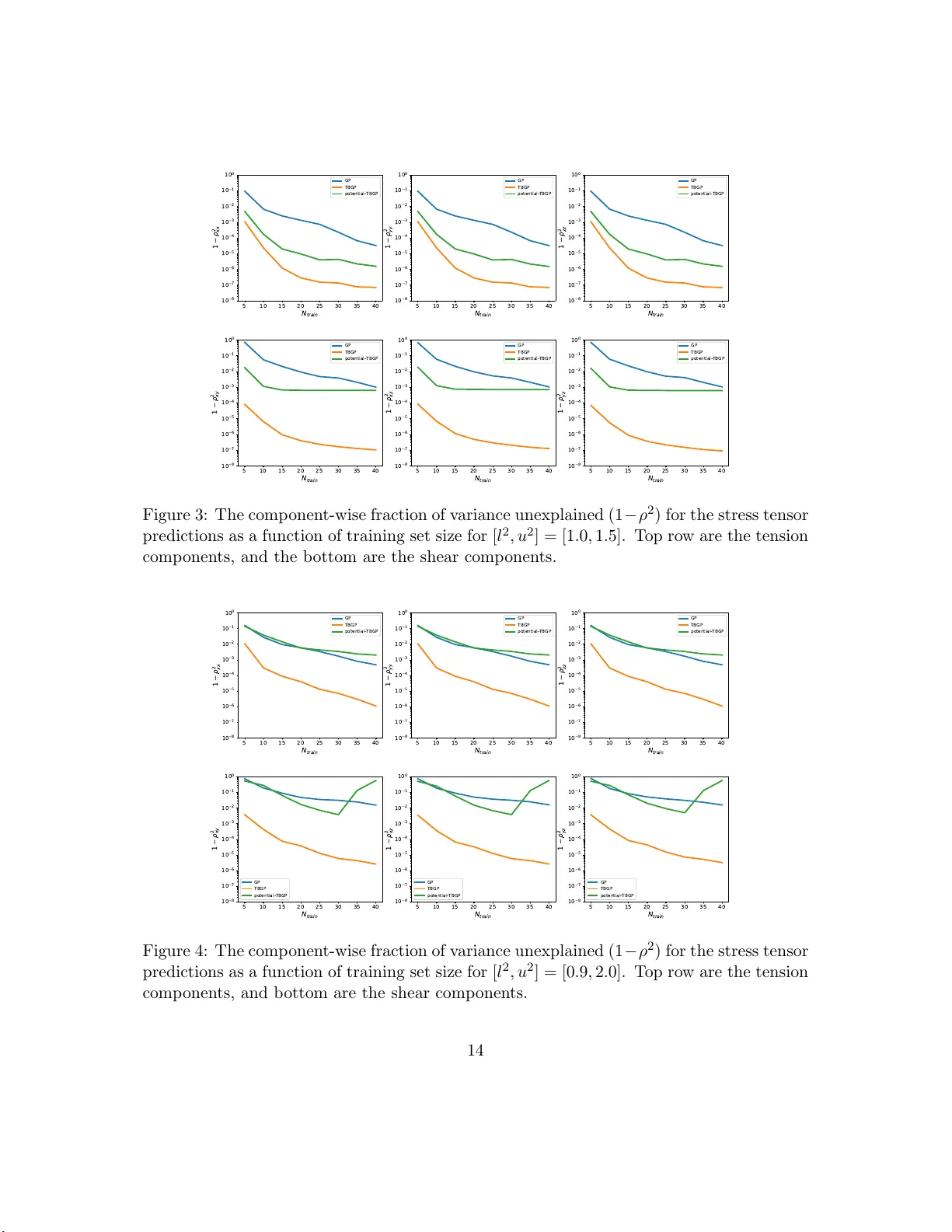
T ensor Basis Gaussian Pro cess Mo dels of Hyp erelastic Materials Ari L. F rank el, Reese E. Jones, Laura P . Swiler Sandia Nationa l L ab or atories Decem b er 24, 2019 Abstract In this work, we dev elop Gaussian pro ces s regressio n ( GPR) mo dels of hyper elastic material b e havior. Firs t, we consider the direct a pproach of mo deling t he comp onents of the Cauch y stress tensor as a function of the comp onents of the Finger stretch tensor in a Gaussian pro cess . W e then consider an improv ement on this approa ch that embeds rotational inv ariance o f the stress-stretch co ns titutiv e r elation in the GPR repre sen- tation. This appro ach r equires few er training examples and achieves hig he r accura cy while maintaining in v ariance to ro tations ex actly . Finally , we consider an a pproach that r ecov ers the stra in-energy density function and derives the str ess tensor fr om this po tent ial. Although the erro r of this mo del for predicting the stress tenso r is higher, the strain-ener g y density is r ecov ered with high accur a cy from limited training data. The approaches presented here are examples of physics-informed machine lear ning. They go beyond purely data-driven approaches b y embedding the physical system constra int s directly in to the Gaussian pro cess represen tation of m ateria ls mo dels. 1 In tro duction Mac hine learning mo dels ha v e seen an explosion in dev elopmen t and applicati on in r ecen t y ears due to their flexibilit y and capacit y for captur in g the trends in complex systems [1]. Pro vided w ith suffi cien t data, the p arameters of the mo d el ma y b e calibrated in suc h a wa y that the mo del giv es high fidelit y repr esentati ons of the u nderlying data generating p r o cess [2, 3, 4, 5]. Moreo v er, computational capabilities hav e gro wn suc h that constru cting deep learning m o dels o v er datasets of tens of th ousands to millions o f d ata p oints is now feasible [6]. There remain, ho w ev er, many applicatio ns in whic h th e amount of data pr esen t is insufficient on its o wn to prop erly train the mac hine learning mo del. This m a y b e du e to a prohibitiv ely large mo del that requires a corresp ondingly large amount of d ata to train and where training data is exp ens ive to acquire. F urthermore, ev en with a we alth of data, it is p ossible t hat the mac hine learning mo del ma y yi eld b eha vior that is inconsistent with the exp ected trend of th e mo d el when the mo del is queried in an extrap ola tory regime. 1 In suc h cases it is app ealing to turn to a framework that allo ws the incorp oratio n of p h ysical p rinciples and other a priori information to sup p lemen t the limited d ata and regularize the b eha vior of the m o del. This inform ation can b e as simple as a kno wn set of constraints th at the regressor must satisfy , such as p ositivit y or monotonicit y with resp ect to a partic ular v ariable, or can b e as complex as kn o wledge of the u nderlying data- generating pro cess in the form of a partial differential equation. Consequent ly , the p ast few y ears ha v e seen great int erest in “physics-constrained” mac hine learning algorithms within the scien tific computing communit y [7, 8, 9, 10, 11, 12, 3]. Th e o v erview pap er b y Karpatne et al. [13] p r o vides a taxonom y for theory-guided data science, with the goal of incorp orating scien tific co nsistency in the learnin g o f generalizable mod els. Muc h researc h in physics-informed mac hine learning h as fo cused on incorp orating constrain ts in neural net w orks [12, 3], often thr ou gh the use of ob jectiv e/loss functions whic h p enalize constraint violatio n [14]. In con trast, the fo cus in th is pap er is to inco rp orate rotational sym metries d irectly and exactly in to Gaussian pro cess repr esen tations of physical resp onse functions. This approac h has the adv an tages of av oiding the bu rden of a large trainin g set that comes with neural net w ork mo del, and the inexact satisfactio n of constrain ts th at come w ith p enaliza tion of constrain ts in the loss function. Th ere h as b een signifi can t in terest in the incorp oration of constrain ts int o Gaussian p ro cess regression mo dels recen tly [15, 16, 17, 18, 2, 19, 20, 21]. Man y of these approac hes leverag e th e analytic f orm ulation of the Gaussian pro cess (GP) to incorp orate constraint s thr ough the lik eliho o d function or the co v ariance function. In this pap er, the task of learning the 6 comp onen ts of a symmetric stress tensor from the 6 comp on ents of a symmetric str etc h tensor is formulate d through a series of transformations so that it b ecomes a regression task of learning three co efficien ts that are a function of three inv ariants of the problem. The main contribution of this pap er is the extension of Gaussian p ro cess regression to enforce rotational in v aria nce through a tensor basis expansion. The pap er is organized as follo ws: Section 2 presen ts an o v erview of constitutive mo dels for h yp erelastic materials. S ections 3 and 4 p resen t Gaussian pro cess regression and the extension to a tensor basis Gaussian pro cess, resp ectiv ely . Sectio n 5 presents a fu rther extension of th e tensor-basis GP to handle the s train en er gy p oten tial. Section 6 pro- vides results for a p articular hyp erelastic Mo oney-Rivlin material, and Section 7 pro vides concluding discussion. 2 Hyp erelastic Materials A hyp erelastic material is a material that remains elastic (non-d iss ipativ e) in the finite/large strain regime. In this con text the fundamental deformation measure is the 3 × 3 deformation gradien t tensor F : F = ∂ x ∂ X , (1) 2 whic h is the d eriv a tiv e of th e current p osition x w ith resp ect to p ositio n X of the same material p oin t in a c hosen reference configuration. In an Eulerian f r ame, the Finger tensor B B = FF T . (2) is the t ypical finite stretc h measure, whic h is directly related to the Almansi str ain, wh ic h measures the total deformation that a material has un dergone r elativ e to its initial config- uration. (The c hoice of the Finger tensor is not limiting in terms of the generalit y of this form ulation, given the equiv ale nce of strain measures pro vided b y the S eth-Hill [22]/Do yle- Eric ksen[23] formulae .) The deform ation of a h yp erelastic material requires an app lied stress state, asso ciated with a certain amoun t of energy , to arrive at that deformed state. F or a hyp erelastic m aterial, the str ess is solely a fun ction of th e current stretc h (or strain) of the material. Hence, the ma jor goal of material mo deling of h yp er elastic materials is to construct constitutiv e relations b et w een the kinematic v ariable B and the corresp onding dynamic v a riable, the 3 × 3 Cauch y stress tensor σ = f ( B ) = 2 I 1 / 2 3 B ∂ Φ ∂ B (3) whic h for a hyper elastic material is giv en by the deriv a tiv e of a p otenti al, namely th e strain energy density Φ. F or fu rther d etails p lease consu lt Refs. [24, 25, 26 ]. T ypical app roac hes to mo d el these relations seek s emi-empirical form ulations for the strain energy density with some parameters to b e fit, which are then fi t to exp erimenta l data. An example of this typ e of formulat ion will b e discussed in a later section. In this w ork w e consider non-parametric mo d eling of hyp erelastic material r esp onses. 3 Gaussian Pro cess Regression Gaussian pro cess regression (GPR) provides a non-parametric mo del f or a resp onse function giv en an inp ut set of training d ata through a Bay e sian up d ate inv olving an assum ed pr ior distribution and a likeli ho o d t ying the p osterior distrib ution to observ ed data. W e denote a Gaussian pro cess prior for a fu nction f b y f ∼ G P (0 , K ) , (4) where we assume the GP has a nominal mean of 0, w ith ou t loss of generalit y , and is de- scrib ed by a cov ariance function K . W e adopt the commonly emplo y ed squared-exp onen tial co v ariance fun ction: K ( x, x ′ ) = θ 1 exp( − θ 2 | x − x ′ | 2 ) (5) whic h has a scale p arameter θ 1 and a length parameter θ 2 . 3 A GP is defined such that any fi nite collection of realizatio ns f rom the pro cess are go v erned b y a m ultiv ariate normal d istribution. T hat is, for any set of observe d realiza- tions X an d pr ediction p oin ts X ∗ with corresp onding f unction v alues f ( X ) and f ( X ∗ ), the probabilit y distrib ution p ( f ( X ∗ ) , f ( X ) | X ∗ , X ) is giv en by  f ( X ) f ( X ∗ )  = N  0 0  ,  K ( X , X ) K ( X , X ∗ ) K ( X ∗ , X ) K ( X ∗ , X ∗ )  (6) where it is und ersto o d that the v ectors and matrices p resen ted are give n in blo c k form for m ultiple instances in X and X ∗ . Gaussian pro cess regression (GPR) uses a GP as a p rior ov er the function space for the data-generating pr o cess, and predictions pro ceed through the use of Bay es’ rule. Up on observ ation of some initial set of noisy data p oin ts y = y ( X ) = f ( X ) + ε with Gaussian noise of v ariance ε 2 in the function v alues, the probabilit y distrib u tion of the v alues of the GP at X ∗ ma y b e determined by form in g the (p osterior) conditional distribution of p ( f ∗ | y , X ): p ( f ∗ | y , X ) = p ( y | f ) p ( f | X ) p ( y | X ) = p ( y | f ) p ( f | X ) R p ( y | f ) p ( f | X )d f (7) where f = f ( X ) and the Gaussian likeli ho o d is giv en by p ( y | f ) = N Y i =1 1 √ 2 π ε 2 exp  − ( y i − f i ) 2 2 ε 2  . (8) This p osterior distribu tion h as the follo wing an alytical solution for the underlying mean pro cess: f ∗ = f ( X ∗ ) ∼ N ( K ∗ ( K + ε 2 I ) − 1 y , K ∗∗ − K ∗ ( K + ε 2 I ) − 1 K ∗ T ) (9) where I den otes the id entit y matrix, K = K ( X , X ), K ∗ = K ( X ∗ , X ), and K ∗∗ = K ( X ∗ , X ∗ ). Then th e predictiv e mean of the d istribution at an y new p oin ts X ∗ is given b y E [ y ∗ ] = K ∗ ( K + ε 2 I ) − 1 y (10) and the predictiv e v ariance, assu ming th e same noise lev el, is giv en b y V [ y ∗ ] = K ∗∗ − K ∗ ( K + ε 2 I ) − 1 K ∗ T + ε 2 I (11 ) where y ∗ = y ( X ∗ ). Th is r esult s h o ws the combinatio n of uncertain t y in the prediction due to epistemic un certain ty in the m ean p ro cess (the fir s t t w o terms on the right side) plus the aleatoric uncertain t y of in herent v ariabilit y in the measurements (the last term on the righ t s id e). In this w ork, although w e will w ork with noiseless d ata, we assum e a v alue of ε 2 = 10 − 10 in order to regularize the inv ersion of the co v ariance matrix. The task th at dominates th e computational exp ense in constructing this mo del is the in v ersion of ( K + ε 2 I ), or, equ iv alen tly , the solution of the linear system based on ( K + ε 2 I ) 4 for either th e m ean or v ariance ev aluations. Since K is dense, th e s caling is typical ly O ( N 3 ) for N training p oin ts. Nominally the matrix is symmetric p ositiv e semi-defin ite, whic h enables efficient solution by Cholesky d ecomp ositio ns, although ill-conditioning is frequent ly an iss u e. Ill-c onditioning r equires adding a rid ge or large noise ( ε ≫ 1) term to the co v ariance matrix to regularize the solution, using ps eu doin v erses via the singular v alue decomp osition (S VD) of the co v ariance matrix, or other greedy subset selection to reduce the matrix size. It app ears at fir s t glance that th e v ariance in Eq. 11 is n omin ally indep enden t of the actual p oin t v alues y , and only dep ends on the lo cations of the selected data p oints X . This is tr u e f or a fixed cov ariance f u nction; ho wev er, we are typica lly in terested in changing the GP hyp erparameters to maximize the accuracy of the GP wh ile balancing th e mo del com- plexit y . T rad itionally , this is managed by tunin g the hyper p arameters to optimize p ( y | X ), whic h is the marginal-lik eliho o d of the GP , and is frequentl y called the “mo del evidence.” Equiv alen tly , we m ay optimize the logarithm of the mo del evidence L = log p ( y | X ) for n umerical stabilit y reasons: L = − 1 2 f T ( K + ε 2 I ) − 1 f − 1 2 log | K + ε 2 I | − N 2 log 2 π (12) That is, we choose to tune the co v ariance hyperp arameters θ 1 and θ 2 in Eq. 5 in order to maximize L . F urth er d iscussion of this appr oac h can b e foun d in Ref. [27]. 4 T ensor Basis Gaussian Pro cess In this section we sho w h o w the standard Gaussian pro cess r egression describ ed in the previous section ma y b e adapted to enforce rotational in v ariance through a tensor basis expansion. W e call this form ulation a tensor basis Gaussian pr o cess (TBGP). 4.1 T ensor Basis E xpansion W e consider the generic hyp erelastic constitutive mo del of the form σ = f ( B ) (13) whic h, for any giv en con tin uous and differentia ble tensor v alued function f , may b e ex- panded in an infin ite series in terms of B w ith fi xed co efficien ts ¯ c n σ = ∞ X n =0 ¯ c n B n (14) It is clear that σ and B are collinear, i.e. ha v e the same eigen basis. Since the tensors of int erest are symmetric and of size 3 × 3, the C a yley-Hamilton theorem states that the tensor B satisfies its corresp ond ing c haracteristic p olynomial B 3 − I 1 B 2 + I 2 B − I 3 I = 0 (15) 5 where w e hav e defin ed the tensor in v arian ts I 1 = tr( B ) = λ B 1 + λ B 2 + λ B 3 , I 2 = 1 2 (tr( B ) 2 − tr( B 2 )) = λ B 1 λ B 2 + λ B 2 λ B 3 + λ B 3 λ B 1 , (16) I 3 = det( B ) = λ B 1 λ B 2 λ B 3 , so-calle d b ecause th ey are inv ariant und er similarit y transformations ( i.e. rotations) of B . Here, λ B 1 , λ B 2 , λ B 3 are the eigen v alues of B , whic h are also a complete set of inv arian ts. The theorem can b e used as a recur s ion r elation to wr ite all p o wers of B higher than 2 in terms of I , B , and B 2 with co efficien ts that dep end on the in v arian ts. Rather than seeking to identify the infin ite n umber of fixed co efficien ts ¯ c i for a giv en constitutiv e r elation, our task reduces to find ing the thr ee co efficien ts in the series expansion σ = c 1 I + c 2 B + c 3 B 2 , (17) where c i is a function of the inv ariants. This r educed expansion main tains rotational ob jectivit y for the original functional de- p enden ce for the app ropriately defined co efficients. T o see this, let R b e an orthogo- nal/rotatio n tensor with inv erse giv en b y R − 1 = R T . The rotation of σ in the original co ordinate frame to the frame d efined by R is give n b y σ ′ ≡ R σ R T = Rf ( B ) R T (18) In v oking the tensor b asis expansion giv es σ ′ = c 1 RIR T + c 2 RBR T + c 3 RB 2 R T (19) = c 1 RR T + c 2 RBR T + c 3 RBR T RBR T = f ( RBR T ) ≡ f ( B ′ ) whic h holds since the eigen v alues, and h ence inv arian ts and the co efficien t functions, do not change up on application of R . In general, an Eulerian tensor fun ction of an Eulerian tensor argument m u st b e ob jectiv e in the sense it resp onds to a rotation of its argument with a corresp ond ing rotation of the fu nction v alue: Rf ( B ) R T = f ( RBR T ) . (20) 4.2 Application t o Gaussian Pro cess Modeling The task of r egression no w falls to learning the co efficients c 1 , c 2 , c 3 as a fun ction of the in v arian ts. This task is compressed from the original pr oblem of h a vin g to learn 6 stress comp onent s f rom 6 strain comp onents with the added b enefit of enforcing the rotatio nal in v ariance that p ro vides this reduction. 6 Supp ose we ha v e b een giv en a dataset of pairs of tensors ( B , σ ). Und er the assum p tion that the tensors ma y b e d iagonaliz ed, the collinearit y of the tensor basis expansion Eq. 17 implies th at they are diagonalize d b y the same eigen vec tor matrix Q bu t with differen t eigen v alue matrices, Λ σ and Λ B , resp ecti ve ly: σ = Q Λ σ Q T (21) B = QΛ B Q T . (22) Then for the give n inpu t-output pair, the v alues of the coefficients for the give n set of eigen v alues are giv en by the solution to a 3 × 3 linear system of equ ations as   λ σ 1 λ σ 2 λ σ 3   =   1 λ B 1 λ 2 B 1 1 λ B 2 λ 2 B 2 1 λ B 3 λ 2 B 3     c 1 c 2 c 3   . (23) This lin ear sys tem ma y b e in ve rted easily to yield the co efficien ts c i ( B , σ ) for eac h training p oint in the dataset, and the inv ariants I i of B ma y also b e computed straigh tforwardly from the eigen v alues giv en in Eq. 16. The three inv ariants I i for eac h observ ation are accum u lated in to a matrix. They take the place of the feature matrix X p resen ted in the previous section and a corresp onding matrix of c i replaces f . W e can thus r eadily extend the GPR approac h to infer the coefficient s as fun ctions of the in v arian ts of the in p ut tensors and thus construct the r ep resen tation of the function σ = c 1 I + c 2 B + c 3 B 2 giv en in Eq. 17. 4.3 Example: Matrix Exp onen tial T o illustrate the impact of em b edd ing rotational inv ariance in the GP formulati on, w e consider the representat ion of the matrix exp onen tial S = exp( B ) = Q exp( Λ ) Q T (24) from a limited n umber of training samples. As in Sec. 4.2, B = QΛQ T is a symmetric diagonaliza ble matrix with eigen v ector matrix Q and diagonal eigen v alue matrix Λ . Clearly the matrix exp onential maintains rotational in v ariance und er application of a rotation R and the series representa tion of exp( B ) demonstr ates the collinearit y of exp( B ) an d B . Giv en Eq. 23, the expansion co efficien ts ma y b e determined from   exp λ 1 exp λ 2 exp λ 3   =   1 λ 1 λ 2 1 1 λ 2 λ 2 2 1 λ 3 λ 2 3     c 1 c 2 c 3   (25) T o create the dataset, we dra w random u niformly distributed 3 × 3 matrices with ent ries b et we en [0 , 1] and compute th eir symmetric p art. A sin gle GP is formed ov er th e 6 inde- p endent tensor comp onen ts (the upp er triangular p art) of B to predict the 6 ind ep endent 7 1 0 1 1 0 2 N 1 0 −8 1 0 −7 1 0 −6 1 0 −5 1 0 −4 1 0 −3 1 0 −2 1 0 −1 1 0 0 R M S E G P te st ro ta te d G P tr a i n T BG P te st ro ta te d T BG P tr a i n Figure 1: The r o ot-mean-squared error in predicting the matrix exp onenti al for the GP and TBGP formulations as a function of training set s ize. The resu lts also show the RMSE of the regressors ev aluated at rand om r otations of the training set pairs. output tensor comp onen ts. This formulatio n is compared against the TBGP formulat ion, where the 3 in v arian ts are used to p redict the 3 expansion co efficients with a single GP . The scikit-le arn library [28] wa s u sed to train th e GPs in b oth cases. The ro ot-mean-squared error is ev aluated in eac h case at 10,000 testing p oints for v alidation. The inp ut tr ainin g p oints are then r otated randomly , and the GP pr ediction is ev aluated at th e inputs. Figure 1 sho ws the results of the testing err or as a function of increasing training p oin ts for the GP and TBGP formulat ions. Since the r otationall y inv ariant form ulation do es n ot tak e the orien tation of the eigen v ectors into account, it is exp ected that the pr ed iction error on the mo dified inputs in this case would b e small, whereas the p rediction error for the normal GP could b e quite large. The T BGP error is indeed 1-2 orders of magnitude lo wer than the GP error on the testing sets, and the error on the r andomly-rotated training set is also o ver 5 orders of magnitude low er, demonstrating that the TBGP f orm ulation learns the u nderlying fun ction m u c h more quic kly th an a standard GP . It also ap p ears to tak e an order of magnitude order more data b efore the GP error catc h es u p to the error that the T BGP h ad on the smallest dataset. Th e error on the rotate d training set app ears to increase, which w e attribute to a com bination of increasing condition num b er of the cov ariance matrix and accumulate d in terp olation error in the GP through the training p oints from the use of regularization to main tain in v ertibilit y . Even with these effects, the TBGP has v ery little er r or throughout the tests and is uniformly the b etter choi ce. 8 5 Strain Energy P oten tial Gaussian Pro cess The tensor basis GP formulation is qu ite p o w erful and could b e made general to m any differen t types of pro cesses. F or h yp erelastic materials, where the stress is the der iv ativ e of a p otent ial, it is p ossible to tak e th is approac h one step fur ther with an alternate form ulation. As in Eq. 3, we defin e th e strain-energy densit y f unction Φ suc h that the stress tensor ma y b e computed as σ = 2 I 1 / 2 3 B ∂ Φ ∂ B (26) for s ome appr opriate Φ( B ). Th e strain-energy densit y is an in v arian t scalar quan tit y an d cannot dep end on the rotation of th e frame; thus for an isotropic h yp erelastic material it is preferable to expr ess the strain-energy d ensit y as a fu nction of the inv ariants of B . Th us the expression for the stress tensor may b e expanded as σ = 2 I 1 / 2 3 B  ∂ Φ ∂ I 1 ∂ I 1 ∂ B + ∂ Φ ∂ I 2 ∂ I 2 ∂ B + ∂ Φ ∂ I 3 ∂ I 3 ∂ B  (27) where w e ha v e applied the c hain rule for the strain-energy densit y partial deriv ativ es. The deriv ativ es of the inv ariants with r esp ect to the original tensor ma y b e compu ted d irectly , refer to Ref. [29], and th e expr ession for σ simplifies to σ = 2 I 1 / 2 3  I 3 ∂ Φ ∂ I 3 I +  ∂ Φ ∂ I 1 + I 1 ∂ Φ ∂ I 2  B − ∂ Φ ∂ I 2 B 2  . (28) This expression explicitly tak es th e form of a tens or-b asis expansion of the type in Eq. 17, where w e hav e c 1 = 2 I 1 / 2 3 ∂ Φ ∂ I 3 c 2 = 2 I 1 / 2 3  ∂ Φ ∂ I 1 + I 1 ∂ Φ ∂ I 2  (29) c 3 = − 2 I 1 / 2 3 ∂ Φ ∂ I 2 F or a giv en set of co efficien ts an d in v arian ts, th e corresp onding partial deriv ativ es can b e ev aluated using the follo wing relations: ∂ Φ ∂ I 1 = I 1 / 2 3 2 ( c 2 + c 3 I 1 ) ∂ Φ ∂ I 2 = − c 3 I 1 / 2 3 2 (30) ∂ Φ ∂ I 3 = c 1 2 I 1 / 2 3 9 Th us giv en a s et of observ ed pairs of ( σ , B ) and Eqs. 23 and 30, w e can infer the cor- resp ond ing v alues of the gradien t of the strain-energy densit y function. F ur thermore, w e “ground” the function ( i.e. remo v e the indeterminacy of calibration of Φ f rom d eriv ativ e data) b y c ho osing a zero-point energy for a set of inv arian ts wh ere the material has not b een deformed. Hence, we augment the gradien t information with the datum Φ( I 1 = 3 , I 2 = 3 , I 3 = 1) = 0 . (31) The GP regression tec hnique can b e extended to tak e adv antag e of deriv ativ e inf or- mation since the deriv ativ e of a GP is also a GP . Sp ecifically , the co v ariance b et ween the deriv ativ es of the s tress-energy densit y b etw een tw o differen t p oin ts in in v ariant sp ace, I = ( I 1 , I 2 , I 3 ) and I ′ = ( I ′ 1 , I ′ 2 , I ′ 3 ), can b e ev aluated as Co v  ∂ Φ( I ) ∂ I i , Φ( I ′ )  = ∂ K ( I , I ′ ) ∂ I i (32) Co v ∂ Φ( I ) ∂ I i , ∂ Φ( I ′ ) ∂ I ′ j ! = ∂ 2 K ( I , I ′ ) ∂ I i ∂ I ′ j (33) Using these relatio ns, a GP ma y b e formed s im ultaneously ov er Φ at th e grounding p oin t and its deriv ativ es ov er the dataset by using the blo c k co v ariance matrix K Φ ( I , I ′ ) =     ∂ 2 K ∂ I 1 ∂ I ′ 1 ∂ 2 K ∂ I 1 ∂ I ′ 2 ∂ 2 K ∂ I 1 ∂ I ′ 3 ∂ 2 K ∂ I 2 ∂ I ′ 1 ∂ 2 K ∂ I 2 ∂ I ′ 2 ∂ 2 K ∂ I 2 ∂ I ′ 3 ∂ 2 K ∂ I 3 ∂ I ′ 1 ∂ 2 K ∂ I 3 ∂ I ′ 2 ∂ 2 K ∂ I 3 ∂ I ′ 3     (34) where eac h en try is a matrix corresp ondin g to the co v ariance b et wee n the ind ividual deriv ativ es of Φ ev aluated b et we en eac h of th e training data p oints. The ground ing p oin t I g = (3 , 3 , 1) is includ ed by augmenting th is m atrix with an add itional r o w and column: K g ( I , I ′ ) =       K ( I g , I g ) ∂ K ( I g , I ′ ) ∂ I ′ 1 ∂ K ( I g , I ′ ) ∂ I ′ 2 ∂ K ( I g , I ′ ) ∂ I ′ 3 ∂ K ( I , I g ) ∂ I 1 ∂ K ( I , I g ) ∂ I 2 K Φ ( I , I ′ ) ∂ K ( I , I g ) ∂ I 3       (35) In a s ligh t abuse of n otatio n, in the matrix K Φ ( I , I ′ ) in Eq . 34 and the matrix K g ( I , I ′ ) in Eq. 35, the arguments I and I ′ should b e interpreted as matrices of the inv ariant s at the training p oints (as opp osed to individual p oints). The GP mean of the p oten tial at a new p oin t I ∗ = ( I ∗ 1 , I ∗ 2 , I ∗ 3 ) ma y then b e predicted with E [Φ( I ∗ )] = K g ( I ∗ , I ) w (36) 10 where w e hav e defin ed the weigh t v ector w = K − 1 g ( I , I ′ ) h 0 ∂ Φ ∂ I 1 ∂ Φ ∂ I 2 ∂ Φ ∂ I 3 i T (37) where the righ t hand side p artial deriv ativ es are at the ob s erv ed data p oin ts, and K g ( I ∗ , I ) is the cov ariance b etw een the test p oin ts and the tr aining p oin ts augmen ted with the groun d p oint. This expression is analogous to Eq. 10, although here we ha ve omitted the noise term. The gradien t of the p otent ial Φ, and hence the stress σ , may b e ev aluated using the same w eigh t vecto r. 6 Results: Mo oney-Rivli n Material In this section w e consider the app licatio n of GPR to predicting d ata dra wn fr om the stress resp onse of the deformation of a h yp erelasti c material. The un derlying tru th mo d el w ill b e assumed to b e a compr essible Mo oney-Rivlin material with s train-energy d en sit y fu nction Φ = c 1 ( I − 1 / 2 3 I 1 − 3) + c 2 ( I − 2 / 3 3 I 2 − 3) + c 3 ( I 1 / 2 3 − 1) 2 (38) where we tak e c 1 = 0 . 162 MP a, c 2 = 0 . 0059 MPa, and c 3 = 10 MPa [30] and w e mak e c 3 ≫ c 1 , c 2 large to effect nearly incompressib le resp onse. W e generate realizatio ns of arbitrary mixed compression/tension/shear states using the follo wing pro cedur e. Let V b e a diagonal matrix of ran d omly sampled p ositiv e v alues b et we en 0 < l ≤ 1 < u , and let R b e a r an d om rotation matrix samp led uniformly on SO(3). W e then emp lo y the p olar decomp osition of the deformation gradient tensor F = R V (39) with corresp ondin g Finger tensor B = R V 2 R T (40) th us guaran teeing that the determinant of F is p ositiv e and that B corresp onds to a v alid diagonalizable tensor with some sup erp osition of tension/compression and sh ear in arbitrary directions. The corresp ond ing eigen v alues of B are r andomly distributed in th e in terv al [ l 2 , u 2 ]. The results shown in Figures 2, 3, and 4 are for tw o d atasets, one sampling [ l 2 , u 2 ] = [1 . 0 , 1 . 5] and another co ve ring [0 . 9 , 2 . 0]. This first c hoice includ es strain v alues corresp ond - ing only to mild extension along the prin cipal axes, w hile the second c hoice includes a more extreme range fr om m ild compression to muc h more extension. The GP , TBGP , and p oten tial-TBGP formulatio ns were trained on 100 differen t rand om samples of datasets of v arying size, and eac h trial’s hyperp arameters w ere selected with multi-sta rt L-BF GS optimization [31] of the marginal like liho o d with 20 rand om initializatio ns. 11 The ro ot-mean-square error is sho w n in Figure 2 and f raction of v ariance un exp lained 1 − ρ 2 for correlation co efficien t ρ for the stress tensor comp onents are sho wn in Figures 3 and 4 as a fu n ction of the training set size f or b oth datasets. It is clear that the T BGP h as a su b stan tially lo w er err or than the GP with app ro ximately the same rate of conv ergence, with 1-2 orders of magnitude low er error and 5-6 orders of magnitude low er unexp lained v ariance. As in the matrix exp onentia l example, the T BGP form ulation is u n iformly the b est c h oice at all tested n umbers of datap oin ts. Ho wev er, the p oten tial-based TBGP has ab out the same error as the regular GP , and b oth show slightly d egraded p erformance on predicting the s h ear comp onen ts of the stress tensor compared to the tension comp onent s. In addition, for larger sets of data the accuracy of p oten tial-TBGP stops impro ving and, in the larger deformation case, the error dive rges. W e attribute this trend to attempting to learn th e fu ll f unction b eha vior fr om gradient inf ormation alone, as w ell as the m uc h larger and more ill-conditioned co v ariance matrix formed in the inference pr o cess. Individual trials of the training pro cess b ecome more lik ely to yield h igher-error mo d els, increasing the a v erage error. It is lik ely that using adv anced low-rank factorizations of the co v ariance matrix or b etter regularization would r ed uce the magnitude of this diverging error. Although th e p oten tial-TBGP p erformance for predicting the stress comp onen ts is no b etter than the GP , it is capable of predicting the strain-energy den s it y function with fairly high accuracy , whic h is not a task that either of the other t w o formulat ions are capable of doing d irectly . F igure 5 sh ows the ro ot-mean-square error and correlation co- efficien t as a function of tr ainin g set size. T h e prediction accuracy do es sho w substantial impro v ement with increasing training d ata f or the lo wer-stretc h case [ l 2 , u 2 ] = [1 . 0 , 1 . 5], but the ill-conditioning issues p rev alen t in the s tr ess pred ictions for the higher-stretc h case [ l 2 , u 2 ] = [0 . 9 , 2 . 0] p erv ad e the p oten tial p rediction as well. Figure 6 shows that the sour ce of d isagreement b etw een the p oten tial-TBGP and the Mo oney-Rivlin p oten tial originates from v alues at higher energy , where there is less data and a more complex trend. One p ossible solution to imp ro v e the p erformance of the p oten tial-TBGP is to use a greedy p oint selection approac h that wo uld use p oin ts th at s pan a wider range of inv ariant space and energy densit y to train the GP . 7 Conclusion This pap er h as develo p ed and demonstrated an approac h to em b edding r otational in- v ariance in the Gaussian pro cess regression f ramew ork for constitutiv e mo d eling of hy- p erelasticit y . Em b edding this physic s k n o wledge led to a dramatic improv ement in the accuracy and learning cu rv es for the TBGP formulat ion compared to the traditional com- p onent based approac h . Al so the p oten tial-TBGP form ulation demonstrated reco very of the p oten tial function from stress-strain data with comparable accuracy to the p lain GP form ulation for stress p rediction. While the examples consider ed here are relativ ely simple, the application of the metho dology to more complex hyp er-elastic materials and f u nctions 12 1 0 2 0 3 0 4 0 N tr a i n 1 0 − 3 1 0 − 2 1 0 − 1 R M S E GP T BGP p o te n t i a l - T BGP 1 0 2 0 3 0 4 0 N tr a i n 1 0 − 2 1 0 − 1 1 0 0 R M S E GP T BGP p o te n t i a l - T BGP Figure 2: The ro ot-mean-squared error o f th e st ress tensor for the GP , T BGP , and p oten tial-TBGP formulations as a function of training set size for [ l 2 , u 2 ] = [1 . 0 , 1 . 5] (upp er panel) and [0 . 9 , 2 . 0] (lo w er panel). 13 5 1 0 1 5 2 0 2 5 3 0 3 5 4 0 N tr a i n 1 0 −8 1 0 −7 1 0 −6 1 0 −5 1 0 −4 1 0 −3 1 0 −2 1 0 −1 1 0 0 1 − ρ 2 x x GP TBGP po te n tia l -TBGP 5 1 0 1 5 2 0 2 5 3 0 3 5 4 0 N t r a in 1 0 −8 1 0 −7 1 0 −6 1 0 −5 1 0 −4 1 0 −3 1 0 −2 1 0 −1 1 0 0 1 − ρ 2 y y GP TBGP po te n t i a l -TBGP 5 1 0 1 5 2 0 2 5 3 0 3 5 4 0 N t ra in 1 0 −8 1 0 −7 1 0 −6 1 0 −5 1 0 −4 1 0 −3 1 0 −2 1 0 −1 1 0 0 1 − ρ 2 zz GP TBGP po te n t i a l -TBGP 5 1 0 1 5 2 0 2 5 3 0 3 5 4 0 N tr a i n 1 0 −8 1 0 −7 1 0 −6 1 0 −5 1 0 −4 1 0 −3 1 0 −2 1 0 −1 1 0 0 1 − ρ 2 x y GP TBGP po te nti a l -TBGP 5 1 0 1 5 2 0 2 5 3 0 3 5 4 0 N t ra in 1 0 −8 1 0 −7 1 0 −6 1 0 −5 1 0 −4 1 0 −3 1 0 −2 1 0 −1 1 0 0 1 − ρ 2 x z GP TBGP p ote n tia l -TBGP 5 1 0 1 5 2 0 2 5 3 0 3 5 4 0 N t ra in 1 0 −8 1 0 −7 1 0 −6 1 0 −5 1 0 −4 1 0 −3 1 0 −2 1 0 −1 1 0 0 1 − ρ 2 y z GP T BGP p o te nti a l -TBGP Figure 3: The comp onen t-wise fraction of v ariance un explained (1 − ρ 2 ) for th e stress tensor predictions as a fu nction of training set size for [ l 2 , u 2 ] = [1 . 0 , 1 . 5]. T op r ow are the tension comp onent s, and th e b ottom are the shear comp onen ts. 5 1 0 1 5 2 0 2 5 3 0 3 5 4 0 N tra in 1 0 −8 1 0 −7 1 0 −6 1 0 −5 1 0 −4 1 0 −3 1 0 −2 1 0 −1 1 0 0 1 − ρ 2 xx GP T BGP p otenti al -T BGP 5 1 0 1 5 2 0 25 3 0 3 5 4 0 N t ra in 1 0 −8 1 0 −7 1 0 −6 1 0 −5 1 0 −4 1 0 −3 1 0 −2 1 0 −1 1 0 0 1 − ρ 2 yy GP T BGP p oten t i a l - TBGP 5 10 1 5 2 0 2 5 3 0 3 5 4 0 N t ra in 1 0 −8 1 0 −7 1 0 −6 1 0 −5 1 0 −4 1 0 −3 1 0 −2 1 0 −1 1 0 0 1 − ρ 2 z z GP T BGP p o t en tia l - TBGP 5 1 0 1 5 2 0 2 5 3 0 3 5 4 0 N trai n 1 0 − 8 1 0 − 7 1 0 − 6 1 0 − 5 1 0 − 4 1 0 − 3 1 0 − 2 1 0 − 1 1 0 0 1 − ρ 2 x y GP TBGP p ote n t i a l - TBGP 5 1 0 1 5 2 0 2 5 3 0 3 5 4 0 N t r a in 1 0 −8 1 0 −7 1 0 −6 1 0 −5 1 0 −4 1 0 −3 1 0 −2 1 0 −1 1 0 0 1 − ρ 2 x z GP TBGP p ote nti a l - TBGP 5 1 0 1 5 2 0 2 5 3 0 3 5 4 0 N t ra in 1 0 −8 1 0 −7 1 0 −6 1 0 −5 1 0 −4 1 0 −3 1 0 −2 1 0 −1 1 0 0 1 − ρ 2 y z GP T BGP p ote nti a l - T BGP Figure 4: The comp onen t-wise fraction of v ariance un explained (1 − ρ 2 ) for th e stress tensor predictions as a fu nction of training set size for [ l 2 , u 2 ] = [0 . 9 , 2 . 0]. T op r ow are the tension comp onent s, and b ottom are the sh ear comp onen ts. 14 5 1 0 1 5 2 0 2 5 3 0 3 5 4 0 N 1 0 − 3 1 0 − 2 1 0 − 1 1 0 0 R M S E 5 1 0 1 5 2 0 2 5 3 0 3 5 4 0 N 1 0 −3 1 0 −2 1 0 −1 1 0 0 R M S E 5 1 0 1 5 2 0 2 5 3 0 3 5 4 0 N 1 0 −8 1 0 −7 1 0 −6 1 0 −5 1 0 −4 1 − ρ 2 5 1 0 1 5 2 0 2 5 3 0 3 5 4 0 N 1 0 −4 1 0 −3 1 0 −2 1 − ρ 2 Figure 5: Th e ro ot-mean-squared error (upp er) and unexplained v ariance (low er) of the strain energy dens ity function Φ as a fun ction of training set size from the p otent ial-TBGP for [ l 2 , u 2 ] = [1 . 0 , 1 . 5] (left) and [ l 2 , u 2 ] = [0 . 9 , 2 . 0] (right). 15 0 1 2 3 4 5 6 Φ tr u e 0 1 2 3 4 5 6 Φ p r e d i c te d 0 5 1 0 1 5 2 0 2 5 3 0 Φ tr u e 0 5 1 0 1 5 2 0 2 5 3 0 Φ p r e d i c te d Figure 6: Scatter-plot of the predicted and actual strain energy densit y v alues at the h ighest training set size for the cases [ l 2 , u 2 ] = [1 . 0 , 1 . 5] (up p er panel) and [0 . 9 , 2 . 0] (lo we r panel). 16 of kinematic v ariables is str aightforw ard. One imp ortan t consideration for future w ork is th e represen tation of anisotropic m a- terial resp onse and functions of multi ple tensors. In these cases, the tensor b asis and corresp ondin g in v ariant s are more complex, bu t the un derlying pr o cess remains the same. F or example, the second Piola-Kirc hoff tensor S ma y b e expressed as a function of the Cauc h y-Green deformation tensor C = F T F and a structure tensor G that c haracterizes the anisotrop y in the resp onse: S = f ( C , G ) (41) (see Ref. [32 ] f or more d etails). F or the case of trans v erse isotropy where the material resp onse along a direction g is different than in the p lane p erp endicular to the unit v ector g , G = g ⊗ g can b e employ ed as the structur e tensor. Th e corresp onding expansion for S is S = 6 X i =1 c i A i (42) in terms of the tensors A i ∈ { I , C , C 2 , G , CG + GC , C 2 G + GC 2 } and co efficien ts c i whic h are functions of the extended inv ariant set { tr C , tr C 2 , tr C 3 , tr CG , tr C 2 G } (refer to Ref. [33] and use G 2 = G ). S ince S is a symmetric tensor and th e tensor basis { A i } is a linearly ind ep endent set, the exp ansion giv es 6 equ ations for the 6 unkn o w ns c i whic h m a y b e solved readily . In this wa y , the corresp onding co efficien ts as a fun ction of the inv arian ts ma y b e inferred and a TBGP ma y b e trained to mak e pr edictions for an anisotropic material resp onse. There is also ro om to impr ov e the p redictions of the p oten tial-based TBGP . Th e squared-exp onential k ernel was selected for its simplicit y an d smo othness, bu t it is p ossib le that a more complex or non-stationary kernel would b e able to capture the b eha vior of the p oten tial fu nction in in v ariant -space more accurately and o v ercome the ill-conditioning issues seen in this formulatio n. Ac kn o wledgmen ts This work w as s upp orted by the LDRD program at S andia National Lab oratories, and its supp ort is gratefully ac knowle dged. Sandia National Lab oratories is a m ultimission lab ora- tory managed and op erated by National T ec hnology and Engineering Solutions of Sandia, LLC., a w holly o wned su bsidiary of Honeywell International, In c., for th e U.S. Departmen t of Energy’s National Nuclear S ecur it y Administration under con tr act d e-na0003 525 . Th e views expressed in the article d o n ot necessarily represent the views of the U.S. Department of En ergy or the United S tates Go v ernment. This man uscrip t has b een deemed UUR with SAND num b er SAND2019-1 5436J. 17 References [1] T rev or Hastie, Rob ert Tibshirani, and Jerome F riedman. The elements of statistic al le arning: data mining, infer enc e and pr e diction, 2nd e d. Sp ringer, 2016. [2] Maziar Raissi, Pa ris Perdik aris, and George EM Karniadakis. Mac hine learning of lin- ear d ifferen tial equations u s ing gaussian p ro cesses. Journal of Computational P hysics , 348:68 3–693, 2017. [3] Reese Jones, Jeremy A T empleton, Cla y M Sanders, and Jak ob T Ostien. Mac hin e learning m o dels of p lastic fl o w based on representa tion theory . Computer Mo deling in Engine ering & Scienc es , pages 309–342, 2018. [4] Ari L F rank el, Reese E Jones, Coleman Alleman, and J erem y A T empleton. Pre- dicting the mechanica l resp on s e of oligocrystals with deep learning. arXiv pr eprint arXiv:1901.10 669 , 2019. [5] Ari F rank el, Kousu ke T ac hida, and Reese Jon es. Pr ed iction of th e ev olution of th e stress field of p olycrystals u ndergoing elastic-plastic deformation with a hybrid neural net w ork mo d el. arXiv pr eprint arXiv:1910.03172 , 2019. [6] Jeffrey Dean, Greg Corr ad o, Ra jat Monga, K ai Chen, Matt hieu Devin, Mark Mao, Marc’aurelio Ranzato, Andrew S enior, P aul T uck er, Ke Y ang, et al. Large scale distributed d eep net wo rks. In A dvanc es in neur al information pr o c essing systems , pages 1223–1 231, 2012. [7] Maziar Raissi an d George EM Karniadakis. Hidden p h ysics m o dels: Mac hine learning of nonlinear partial d ifferen tial equations. Journal of Computational Physics , 357:125– 141, 2018. [8] S. P an and K. Du r aisam y . Data-driv en disco v ery of closure mo dels. SIAM Journal on Applie d Dynamic al Systems , 17(4):23 81–2413, 2018. [9] B. Lusch, J. N. Kutz, and S. L. Brunt on. Deep learning for universal linear em b edd ings of n onlinear dynamics. N atur e Communic ations , 9(1):4950 , 2018. [10] S . L. Brunton, J. L. Pro ctor, and J . N. Kutz. Disco vering go v erning equations from data b y sp arse id en tification of nonlinear dynamical s y s tems. P r o c e e dings of the Na- tional A c ademy of Scienc es , 113(15):3 932–39 37, 2016. [11] K o okjin Lee and Kevin C arlb erg. Mo d el red u ction of dyn amical s y s tems on n onlinear manifolds using deep conv olutional autoenco d ers. arXiv pr eprint arXiv:1812.08373 , 2018. 18 [12] J ulia Ling, Reese Jones, and J erem y T emp leton. Mac hine learning s tr ategie s for sys- tems with inv ariance prop erties. Journal of Computa tional Physics , 318:2 2–35, 2016. [13] Anuj Karpatne, Go wtham A tluri, James H F aghmous, Mic h ael S tein bac h, Arindam Banerjee, Auro op Ganguly , Shashi S hekhar, Nagiza S amato v a, and Vipin Ku m ar. Theory-guided data science: A new paradigm for scien tific discov ery from data. IE EE T r ansactions on Know le dge and Data Eng i ne ering , 29(10) :2318–2 331, 2017. [14] J im Magiera, Deep Ra y , Jan S Hestha v en, and Christian Rohde. Constraint -a w are neural net w orks for r iemann problems. arXiv pr eprint arXiv:1904.12794 , 2019. [15] J aakk o Riihim¨ aki and Aki V ehta ri. Gaussian pro cesses with m onotonicit y information. In P r o c e e dings of the Thirte enth International Confer enc e on Artificial Intel ligenc e and Statistics , pages 645–652 , 2010. [16] S´ ebastien Da V eiga and Amandin e Marrel. Gauss ian pro cess mo deling with inequalit y constrain ts. In Annales de la F acult ´ e des Scienc es de T oulouse , vo lume 21, pages 529– 555, 2012. [17] Bjørn San d Jensen, Jens Brehm Nielsen, and Jan Larsen. Bounded gaussian pro cess regression. In 2013 IE EE International Workshop on Machine L e arning for Signal Pr o c essing (M LSP) , p ages 1–6. IEEE, 2013. [18] E rcan Solak, Ro derick Murray-Smith, William E Leithead, Douglas J Leith, and Carl E Rasm u s sen. Deriv ativ e ob s erv ations in gaussian p ro cess mo dels of dynamic systems. In A dvanc es in neur al information pr o c essing systems , pages 1057–1064 , 2003. [19] Xiu Y ang, Guzel T artako vsky , and Alexandre T artak o vsk y . Physics-informed kriging: A ph ysics-informed gaussian pro cess regression metho d for data-mod el con verge nce. arXiv pr eprint arXiv:1809.0 3461 , 2018. [20] An dr´ es F L´ op ez-Lopera, F ran¸ cois Bac h o c, Nicolas Dur r ande, and Olivier Rous- tan t. Finite-dimensional gaussian appro ximation with linear inequalit y constraints. SIAM/ASA J ournal on U nc ertainty Quantific ation , 6(3):1224– 1255, 2018. [21] F ran¸ cois Bac ho c, Agnes L agnoux, Andr´ es F L´ op ez-Lop era, et al. Maxim um lik eliho o d estimation for gaussian pro cesses und er inequalit y constraints. Ele ctr onic Journal of Statistics , 13(2):29 21–2969 , 2019. [22] R Hill. On constitutiv e inequalities for simple materialsi. Journ al of the Me chanics and P hysics of Solids , 16(4):229– 242, 1968 . [23] T C Do yle and Jerald L Eric ksen. Nonlinear elasticit y . In A dvanc es i n applie d me chan- ics , volume 4, p ages 53–115. Elsevier, 1956. 19 [24] L E Malve rn. In tro duction to con tinuum mechanics. Pr entic e Hal l Inc., Engle Cliffs, NJ , 1696:3 01–320, 1969. [25] R aymond W O gden. Non-line ar elastic deformations . Courier Corp oration, 1997. [26] Morton E Gur tin. An intr o duction to c ontinuum me chanics , v olume 158 . Academic press, 1982. [27] C arl Edward Rasm u ssen and Christopher KI Williams. Gaussian Pr o c esses for Ma- chine L e arning . MIT Press, 2006. [28] F. Pedregosa , G. V aro quaux, A. Gramfort, V. Mic hel, B. Thirion, O. Grisel, M. Blon- del, P . Prettenhofer, R. W eiss, V. Dub ourg, J. V anderplas, A. P assos, D. Cou r nap eau, M. Brucher, M. Perrot, and E. Duc hesnay . Scikit-learn: Mac hine learning in Python. Journal of M achine L e arning R ese ar ch , 12:282 5–2830, 2011. [29] J a v ier Bonet and Richard D W o o d. Nonline ar c ontinuum me chanics for finite element analysis . Cambridge un iversit y p ress, 1997. [30] Gilles Marckmann and Er w an V erron. Comparison of hyperelastic mo d els for r u bb er- lik e materials. Rubb er chemistry and te c hnolo gy , 79(5):83 5–858, 2006. [31] R . Byrd, P . Lu , and J. Nocedal. A limited memory algorithm for b ound constrained optimization. SIAM Journal on Scientific and Statistic al Computing , 16:1190– 1208, 1995. [32] Q -S Zh eng. Theory of repr esen tations for tensor functionsa unifi ed inv ariant approac h to constitutiv e equations. Applie d Me chanics R eviews , 47(11):545– 587, 1994. [33] J P Bo ehler. Representat ions for isotropic and anisotropic non -p olynomial tensor f unc- tions. In Applic ations of tensor fu nctions in solid me chanics , p ages 31–53 . Spr inger, 1987. 20