More Data Can Hurt for Linear Regression: Sample-wise Double Descent

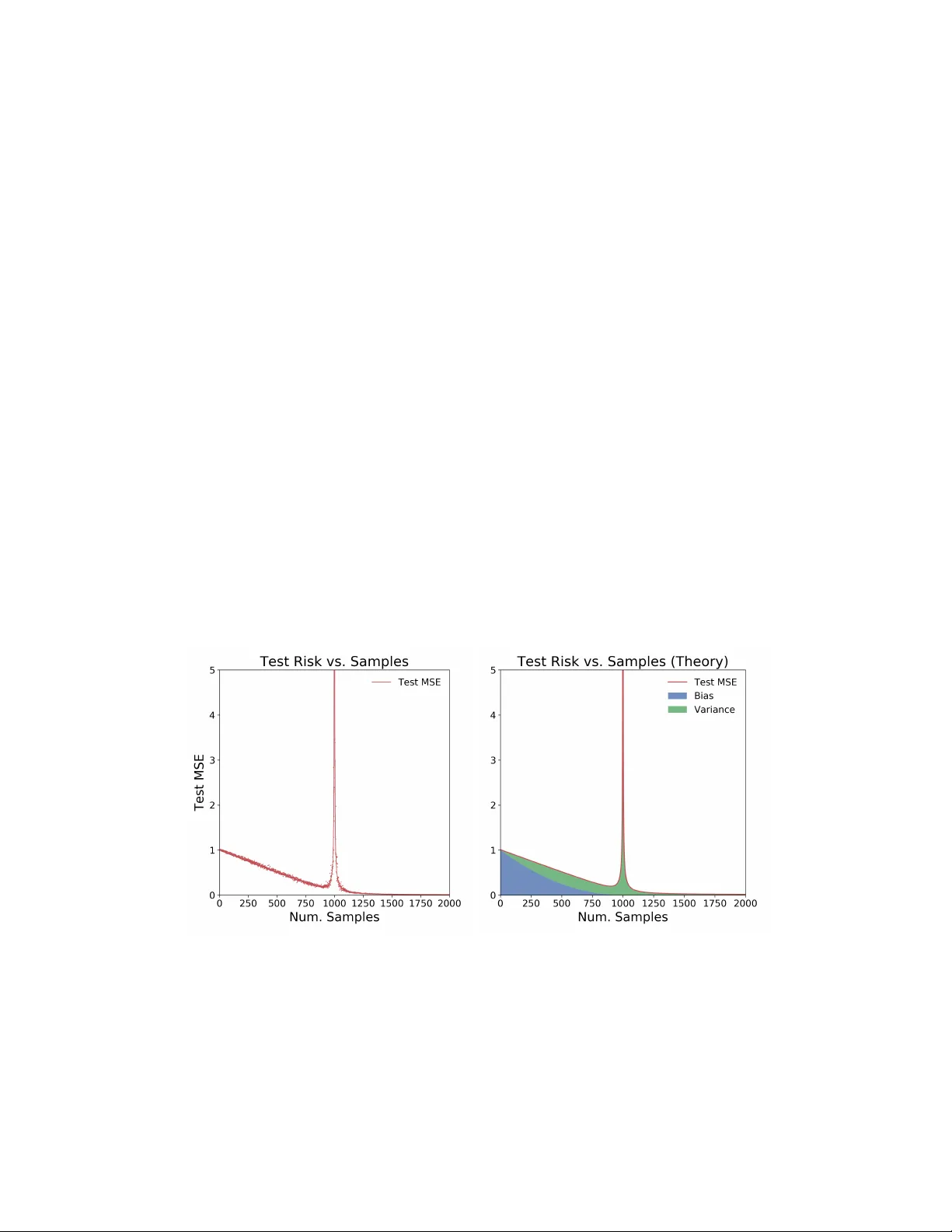
More Data Can Hurt for Linear Regression: Sample-wise Double Descen t Preetum Nakkiran Harv ard Univ ersit y Abstract In this exp ository note w e describ e a surprising phenomenon in ov erparameterized linear regression, where the dimension exceeds the n umber of samples: there is a regime where the test risk of the estimator found by gradient descent incr e ases with additional samples. In other words, more data actually hurts the estimator. This behavior is implicit in a recen t line of theoretical works analyzing “double descent” phenomena in linear mo dels. In this note, w e isolate and understand this b ehavior in an extremely simple setting: linear regression with isotropic Gaussian cov ariates. In particular, this o ccurs due to an uncon ven tional t yp e of bias-varianc e tr ade off in the o verparameterized regime: the bias decreases with more samples, but v ariance incr e ases . 1 In tro duction Common statistical in tuition suggests that more data should never harm the p erformance of an estimator. It w as recently highligh ted in [Nakkiran et al., 2019] that this may not hold for overp ar ameterize d mo dels: there are settings in mo dern deep learning where training on more data actually h urts. In this note, we analyze a simple setting to understand the mec hanisms behind this behavior. (a) T est MSE for d = 1000 , σ = 0 . 1 . (b) T est MSE in theory for d = 1000 , σ = 0 . 1 Figure 1: T est MSE vs. Num. T rain Samples for the min-norm ridgeless regression estimator in d = 1000 dimensions. The distribution is a linear model with noise: co v ariates x ∼ N (0 , I d ) and response y = h x, β i + N (0 , σ 2 ) , for d = 1000 , σ = 0 . 1 , and || β || 2 = 1 . The estimator is ˆ β = X † y . L eft: Solid line sho ws mean o ver 50 trials, and individual p oin ts show a single trial. Right: Theoretical predictions for the bias, v ariance, and risk from Claims 1 and 2. 1 W e fo cus on well-specified linear regression with Gaussian cov ariates, and we analyze the test risk of the minim um-norm ridgeless regression estimator— or equiv alently , the estimator found b y gradien t descen t on the least squares ob jective. W e sho w that as w e increase the num b er of samples, p erformance is non- monotonic: The test risk first decreases, and then incr e ases , before decreasing again. Suc h a “double-descent” b ehavior has b een observed in the b ehavior of test risk as a function of the mo del size in a v ariety of mac hine learning settings [Opp er, 1995, Opp er, 2001, A dv ani and Saxe, 2017, Belkin et al., 2018, Spigler et al., 2018, Geiger et al., 2019, Nakkiran et al., 2019]. Man y of these works are motiv ated b y understanding the test risk as function of mo del size, for a fixed num b er of samples. In this w ork, w e take a complemen tary view and understand the test risk as a function of sample size , for a fixed mo del. W e hope that understanding suc h simple settings can even tually lead to understanding the general phenomenon, and lead us to design learning algorithms which make the b est use of data (and in particular, are monotonic in samples). W e note that similar analyses app ear in recen t works, whic h we discuss in Section 1.1– our fo cus is to highligh t the sample non-monotonicit y implicit in these works, and give intuitions for the mec hanisms behind it. W e sp ecifically refer the reader to [Hastie et al., 2019, Mei and Montanari, 2019] for analysis in a setting most similar to ours. Organization. W e first define the linear regression setting in Section 2. Then in Section 3 we state the form of the estimator found by gradient descent, and give intuitions for wh y this estimator has a p eak in test risk when the num b er of samples is equal to the am bien t dimension. In Section 3.1, we decomp ose the exp ected excess risk into bias and v ariance contributions, and we state appro ximate expressions for the bias, v ariance, and excess risk as a function of samples. W e sho w that these appro ximate theoretical predictions closely agree with practice, as in Figure 1. The peak in test risk turns out to b e related to the conditioning of the data matrix, and in Section 3.2 w e give intuitions for why this matrix is p o orly conditioned in the “critical regime”, but well conditioned outside of it. W e also analyze the marginal effect of adding a single sample to the test risk, in Section 3.3. W e conclude with discussion and op en questions in Section 4. 1.1 Related W orks This work was inspired by the long line of w ork studying “double descen t” phenomena in deep and shallow mo dels. The general principle is that as the mo del complexity increases, the test risk of trained mo dels first decreases and then increases (the standard U-shape), and then de cr e ases again . The peak in test risk o ccurs in the “critical regime” when the mo dels are just barely able to fit the training set. The second descen t o ccurs in the “o v erparameterized regime”, when the model capacit y is large enough to con tain sev eral interpolants on the training data. This phenomenon app ears to b e fairly universal among natural learning algorithms, and is observed in simple settings such as linear regression, random features regres- sion, classification with random forests, as well as mo dern neural netw orks. Double descent of test risk with model size was introduced in generalit y b y [Belkin et al., 2018], building on similar behavior observed as early as [Opp er, 1995, Opp er, 2001] and more recently by [Adv ani and Saxe, 2017, Neal et al., 2018, Spigler et al., 2018, Geiger et al., 2019]. A generalized double descent phenomenon w as demonstrated on mo dern deep net w orks b y [Nakkiran et al., 2019], which also highligh ted “sample-wise nonmonotonicity” as a consequence of double descen t – showing that more data can hurt for deep neural net works. A num b er of recen t works theoretically analyze the double descent behavior in simplified settings, often for linear mo dels [Belkin et al., 2019, Hastie et al., 2019, Bartlett et al., 2019, Muthukumar et al., 2019, Bibas et al., 2019, Mitra, 2019, Mei and Montanari, 2019, Liang and Rakhlin, 2018, Liang et al., 2019, Xu and Hsu, 2019, Dereziński et al., 2019, Lampinen and Ganguli, 2018, Deng et al., 2019]. A t a high lev el, 2 these works analyze the test risk of estimators in ov erparameterized linear regression with different assump- tions on the cov ariates. W e sp ecifically refer the reader to [Hastie et al., 2019, Mei and Montanari, 2019] for rigorous analysis in a setting most similar to ours. In particular, [Hastie et al., 2019] considers the asymptotic risk of the minimum norm ridgeless regression estimator in the limit where dimension d and n umber of samples n are scaled as d → ∞ , n = γ d . W e instead fo cus on the sample-wise p ersp ective: a fixed large d , but v arying n . In terms of technical conten t, the analysis technique is not no v el to our work, and similar calculations appear in some of the prior works ab ov e. Our main contribution is highligh ting the sample non-monotonic behavior in a simple setting, and elab orating on the mec hanisms resp onsible. While man y of the abov e theoretical results are qualitativ ely similar, w e highligh t one interesting distinc tion: our setting is wel l-sp e cifie d , and the bias of the estimator is monotone nonincreasing in n umber of samples (see Equation 3, and also [Hastie et al., 2019, Section 3]). In con trast, for missp e cifie d problems (e.g. when the ground-truth is nonlinear, but we learn a linear model), the bias can actually increase with num b er of samples in addition to the v ariance increasing (see [Mei and Montanari, 2019]). 2 Problem Setup Consider the following learning problem: The ground-truth distribution D is ( x, y ) ∈ R d × R with cov ariates x ∼ N (0 , I d ) and resp onse y = h x, β i + N (0 , σ 2 ) for some unknown, arbitrary β such that || β || 2 ≤ 1 . That is, the ground-truth is an isotropic Gaussian with observ ation noise. W e are given n samples ( x i , y i ) from the distribution, and we w ant to learn a linear mo del f ˆ β ( x ) = h x, ˆ β i for estimating y given x . That is, we w ant to find ˆ β with small test mean squared error R ( ˆ β ) := E ( x,y ) ∼D [( h x, ˆ β i − y ) 2 ] = || ˆ β − β || 2 + σ 2 (for isotropic x ∼ N (0 , I d ) ) Supp ose we do this b y p erforming ridgeless linear regression. Sp ecifically , we run gradien t descen t initialized at 0 on the follo wing objective (the empirical risk). min ˆ β || X ˆ β − y || 2 (1) where X ∈ R n × d is the data-matrix of samples x i , and y ∈ R n are the observ ations. The solution found by gradien t descent at conv ergence is ˆ β = X † y , where † denotes the Mo ore–Penrose pseudoin verse 1 . Figure 1a plots the exp ected test MSE of this estimator E X,y [ R ( ˆ β ))] as w e v ary the num b er of train samples n . Note that it is non-monotonic, with a peak in test MSE at n = d . There are t wo surprising aspects of the test risk in Figure 1a, in the ov erparameterized regime ( n < d ): 1. The first descen t: where test risk initially decreases even when we hav e less samples n than dimen- sions d . This o ccurs b ecause the bias decreases. 2. The first ascent: where test risk increases, and peaks when n = d . This is because the v ariance increases, and div erges when n = d . When n > d , this is the classical underparameterized regime, and test risk is monotone decreasing with n umber of samples. Th us o v erparameterized linear regression exhibits a bias-varianc e tr ade off : bias decreases with more samples, but v ariance can increase. Belo w, we elaborate on the mec hanisms and pro vide in tuition for this non- monotonic b ehavior. 1 T o see this, notice that the iterates of gradient descent lie in the row-space of X . 3 3 Analysis The solution found by gradien t descent, ˆ β = X † y , has different forms dep ending on the ratio n/d . When n ≥ d , w e are in the “underparameterized” regime and there is a unique minimizer of the objective in Equation 1. When n < d , w e are “o verparameterized” and there are man y minimizers of Equation 1. In fact, since X is full rank with probability 1, there are many minimizers which interp olate , i.e. X ˆ β = y . In this regime, gradien t descent finds the minimum with smallest ` 2 norm || ˆ β || 2 . That is, the solution can be written as ˆ β = X † y =      argmin β : X β = y || β || 2 when n ≤ d (“Ov erparameterized”) argmin β || X β − y || 2 when n > d (“Underparameterized”) The ov erparameterized form yields insigh t into wh y the test MSE p eaks at n = d . Recall that the observ ations are noisy , i.e. y = X β + η where η ∼ N (0 , σ 2 I n ) . When n  d , there are many interpolating estimators { ˆ β : X ˆ β = y } , and in particular there exist such ˆ β with small norm. In con trast, when n = d , there is exactly one interpolating estimator ( X ˆ β = y ) , but this estimator must hav e high norm in order to fit the noise η . More precisely , consider ˆ β = X † y = X † ( X β + η ) = X † X β | {z } signal + X † η | {z } noise The signal term X † X β is simply the orthogonal pro jection of β on to the rows of X . When we are “critically parameterized” and n ≈ d , the data matrix X is very p o orly conditioned, and hence the noise term X † η has high norm, ov erwhelming the signal. This argument is made precise in Section 3.1, and in Section 3.2 we giv e in tuition for wh y X b ecomes p o orly conditioned when n ≈ d . The main p oint is that when n = d , forcing the estimator ˆ β to interpolate the noise will force it to hav e very high norm, far from the ground-truth β . (See also Corollary 1 of [Hastie et al., 2019] for a quan tification of this p oint). 3.1 Excess Risk and Bias-V ariance T radeoffs F or ground-truth parameter β , the excess risk 2 of an estimator ˆ β is: R ( ˆ β ) := E ( x,y ) ∼D [( h x, ˆ β i − y ) 2 ] − E ( x,y ) ∼D [( h x, β i − y ) 2 ] = E x ∼N (0 ,I ) ,η ∼N (0 ,σ 2 ) [( h x, ˆ β i − h x, β i + η ) 2 ] − σ 2 = || ˆ β − β || 2 F or an estimator ˆ β X,y that is deriv ed from samples ( X , y ) ∼ D n , w e consider the exp ected excess risk of ˆ β = ˆ β X,y in exp ectation o ver samples ( X, y ) : E X,y [ R ( ˆ β X,y )] = E X,y [ || ˆ β − β || 2 ] = || β − E [ ˆ β ] || 2 | {z } Bias B n + E [ || ˆ β − E [ ˆ β ] || 2 ] | {z } V ariance V n (2) Where B n , V n are the bias and v ariance of the estimator on n samples. 2 F or clarity , we consider the excess risk, which omits the unav oidable additive σ 2 error in the true risk. 4 F or the sp ecific estimator ˆ β = X † y in the regime n ≤ d , the bias and v ariance can b e written as (see App endix A.1): B n = || E X ∼D n [ Pro j X ⊥ ( β )] || 2 (3) V n = E X [ || Pro j X ( β ) − E X [ Pro j X ( β )] || 2 ] | {z } ( A ) + σ 2 E X [T r  ( X X T ) − 1  ] | {z } ( B ) (4) where Proj X is the orthogonal projector on to the rowspace of the data X ∈ R n × d , and Proj X ⊥ is the pro jector onto the orthogonal complemen t of the rowspace. F rom Equation 3, the bias is non-increasing with samples ( B n +1 ≤ B n ), since an additional sample can only gro w the rowspace: X ⊥ n +1 ⊆ X ⊥ n . The v ariance in Equation 4 has tw o terms: the first term (A) is due to the randomness of X , and is bounded. But the second term (B) is due to the randomness in the noise of y , and div erges when n ≈ d since X b ecomes p o orly conditioned. This trace term is resp onsible for the peak in test MSE at n = d . W e can also approximately compute the bias, v ariance, and excess risk. Claim 1 (Ov erparameterized Risk) . L et γ := n d < 1 b e the underp ar ameterization r atio. The bias and varianc e ar e: B n = (1 − γ ) 2 || β || 2 (5) V n ≈ γ (1 − γ ) || β || 2 + σ 2 γ 1 − γ (6) A nd thus the exp e cte d exc ess risk for γ < 1 is: E [ R ( ˆ β )] ≈ (1 − γ ) || β || 2 + σ 2 γ 1 − γ (7) = (1 − n d ) || β || 2 + σ 2 n d − n (8) These appro ximations are not exact because they hold asyptotically in the limit of large d (when scal- ing n = γ d ), but ma y deviate for finite samples. In particular, the bias B n and term (A) of the v ari- ance can be computed exactly for finite samples: Pro j X is simply a pro jector onto a uniformly random n -dimensional subspace, so E [ Pro j X ( β )] = γ β , and similarly E [ || Pro j X ( β ) || 2 ] = γ || β || 2 . The trace term (B) is non trivial to understand for finite samples, but conv erges 3 to γ 1 − γ in the limit of large n, d (e.g. Lemma 3 of [Hastie et al., 2019]). In Section 3.3, we give intuitions for why the trace term con verges to this. F or completeness, the bias, v ariance, and excess risk in the underparameterized regime are giv en in [Hastie et al., 2019, Theorem 1] as: Claim 2 (Underparameterized Risk, [Hastie et al., 2019]) . L et γ := n d > 1 b e the underp ar ameterization r atio. The bias and varianc e ar e: B n = 0 , V n ≈ σ 2 γ − 1 Figure 1 sho ws that Claims 1 and 2 agree with the excess risk experimentally even for finite d = 1000 . 3 F or large d , the sp ectrum of ( X X T ) is understoo d by the Marchenk o–Pastur law [Marčenko and Pastur, 1967]. Lemma 3 of [Hastie et al., 2019] uses this to show that T r  ( X X T ) − 1  → γ 1 − γ . 5 3.2 Conditioning of the Data Matrix Here we give intuitions for wh y the data matrix X ∈ R n × d is well conditioned for n  d , but has small singular v alues for n ≈ d . 3.2.1 Near Criticality First, let us consider the effect of adding a single sample when n = ( d − 1) . F or simplicity , assume the first ( d − 1) samples x i are just the standard basis vectors, scaled appropriately . That is, assume the data matrix X ∈ R ( d − 1) × d is X =  dI d − 1 0  . This has all non-zero singular v alues equal to d . Then, consider adding a new isotropic Gaussian sample x n +1 ∼ N (0 , I d ) . Split this into co ordinates as x n +1 = ( g 1 , g 2 ) ∈ R d − 1 × R . The new data matrix is X n +1 =  dI d − 1 0 g 1 g 2  W e claim that X n +1 has small singular v alues. Indeed, consider left-multiplication by v T :=  g 1 − d  : v T X n +1 =  g 1 − d   dI d − 1 0 g 1 g 2  =  0 − dg 2  Th us, || v T X n +1 || 2 ≈ d 2 , while || v || 2 ≈ 2 d 2 . Since X n +1 is full-rank, it must hav e a singular v alue less than roughly 1 √ 2 . That is, adding a new sample has shrunk the minimum non-zero singular v alue of X from d to less than a constant. The intuition here is: although the new sample x n +1 adds rank to the existing samples, it do es so in a very fragile wa y . Most of the ` 2 mass of x n +1 is contained in the span of existing samples, and x n only contains a small comp onen t outside of this subspace. This causes X n +1 to hav e small singular v alues, whic h in turn causes the ridgeless regression estimator (which applies X † ) to be sensitiv e to noise. A more careful analysis shows that the singular v alues are actually ev en smaller than the ab ov e simplification suggests — since in the real setting, the matrix X w as already p o orly conditioned even b efore the new sample x n +1 . In Section 3.3 w e calculate the exact effect of adding a single sample to the excess risk. 3.2.2 F ar from Criticality When n  d , the data matrix X do es not ha ve singular v alues close to 0 . One wa y to see this is to notice that since our data mo del treats features and samples symmetrically , X is well conditioned in the regime n  d for the same reason that standard linear regression w orks in the classical underparameterized regime n  d (b y “transp osing” the setting). More precisely , since X is full rank, its smallest non-zero singular v alue can b e written as σ min ( X ) = min v ∈ R n : || v || 2 =1 || v T X || 2 Since X has en tries i.i.d N (0 , 1) , for every fixed v ector v w e ha ve E X [ || v T X || 2 ] = d || v || 2 = d . Moreo ver, for d = Ω( n ) uniform conv ergence holds, and || v T X || 2 concen trates around its exp ectation for all vectors v in the ` 2 ball. Thus: σ min ( X ) 2 ≈ E X  min v ∈ R n : || v || 2 =1 || v T X || 2  ≈ min v E X [ || v T X || 2 ] = d 6 3.3 Effect of A dding a Single Sample Here we show how the trace term of the v ariance in Equation 4 changes with increasing samples. Sp ecifically , the following claim shows how T r  ( X X T ) − 1  gro ws when we add a new sample to X . Claim 3. L et X ∈ R n × d b e the data matrix after n samples, and let x ∈ R d b e the ( n + 1) th sample. The new data matrix is X n +1 =  X x T  , and T r  ( X n +1 X T n +1 ) − 1  = T r  ( X X T ) − 1  + 1 + || ( X T ) † x || 2 || Pro j X ⊥ ( x ) || 2 Pr o of. By computation in App endix A.2. If we heuristically assume the denominator concentrates around its exp ectation, || Pro j X ⊥ ( x ) || 2 ≈ d − n , then w e can use Claim 3 to estimate the exp ected effect of a single sample: E x T r  ( X n +1 X T n +1 ) − 1  ≈ T r  ( X X T ) − 1  + 1 + E x || ( X X T ) − 1 X x || 2 d − n (9) = T r  ( X X T ) − 1   1 + 1 d − n  + 1 d − n (10) W e can further estimate the growth b y taking a contin uous limit for large d . Let F ( n d ) := E [T r  ( X n X T n ) − 1  ] . Then for γ := n d , Equation 10 yields the differential equation dF ( γ ) dγ = (1 − γ ) − 1 F + (1 − γ ) − 1 whic h is solved by F ( γ ) = γ 1 − γ . This heuristic deriv ation that E [T r  X X T  − 1 ] → γ 1 − γ is consistent with the rigorous asymptotics giv en in [Hastie et al., 2019, Lemma 3] and used in Claim 1. 4 Discussion W e hop e that understanding such simple settings can even tually lead to understanding the general b ehavior of o verparameterized mo dels in mac hine learning. W e consider it extremely unsatisfying that the most p opular technique in mo dern machine learning (training an ov erparameterized neural net work with SGD) can be nonmonotonic in samples [Nakkiran et al., 2019]. W e hop e that a greater understanding here could help dev elop learning algorithms which mak e the best use of data (and in particular, are monotonic in samples). In general, w e believe it is interesting to understand when and why learning algorithms are monotonic – esp ecially when w e don’t explicitly enforce them to b e. A c knowledgemen ts W e esp ecially thank Jacob Steinhardt and Aditi Raghunathan for discussions and suggestions that motiv ated this work. W e thank Jarosław Błasiok, Jonathan Shi, and Boaz Barak for useful discussions throughout this w ork, and we thank Gal Kaplun and Benjamin L. Edelman for feedback on an early draft. This work supp orted in part b y supp orted b y NSF aw ards CCF 1565264, CNS 1618026, and CCF 1715187, a Simons In vestigator F ellowship, and a Simons Inv estigator A w ard. 7 References [A dv ani and Saxe, 2017] A dv ani, M. S. and Saxe, A. M. (2017). High-dimensional dynamics of generalization error in neural netw orks. arXiv pr eprint arXiv:1710.03667 . [Bartlett et al., 2019] Bartlett, P . L., Long, P . M., Lugosi, G., and T sigler, A. (2019). Benign ov erfitting in linear regression. arXiv pr eprint arXiv:1906.11300 . [Belkin et al., 2018] Belkin, M., Hsu, D., Ma, S., and Mandal, S. (2018). Reconciling modern mac hine learning and the bias-v ariance trade-off. arXiv pr eprint arXiv:1812.11118 . [Belkin et al., 2019] Belkin, M., Hsu, D., and Xu, J. (2019). T wo mo dels of double descent for weak features. arXiv pr eprint arXiv:1903.07571 . [Bibas et al., 2019] Bibas, K., F ogel, Y., and F eder, M. (2019). A new look at an old problem: A univ ersal learning approach to linear regression. arXiv pr eprint arXiv:1905.04708 . [Deng et al., 2019] Deng, Z., Kammoun, A., and Thrampoulidis, C. (2019). A mo del of double descent for high-dimensional binary linear classification. arXiv pr eprint arXiv:1911.05822 . [Dereziński et al., 2019] Dereziński, M., Liang, F., and Mahoney , M. W. (2019). Exact expressions for double descen t and implicit regularization via surrogate random design. [Geiger et al., 2019] Geiger, M., Spigler, S., d’Ascoli, S., Sagun, L., Baity-Jesi, M., Biroli, G., and W yart, M. (2019). Jamming transition as a paradigm to understand the loss landscap e of deep neural netw orks. Physic al R eview E , 100(1):012115. [Hastie et al., 2019] Hastie, T., Montanari, A., Rosset, S., and Tibshirani, R. J. (2019). Surprises in high- dimensional ridgeless least squares in terp olation. [Lampinen and Ganguli, 2018] Lampinen, A. K. and Ganguli, S. (2018). An analytic theory of generalization dynamics and transfer learning in deep linear net works. arXiv pr eprint arXiv:1809.10374 . [Liang and Rakhlin, 2018] Liang, T. and Rakhlin, A. (2018). Just in terp olate: Kernel" ridgeless" regression can generalize. arXiv pr eprint arXiv:1808.00387 . [Liang et al., 2019] Liang, T., Rakhlin, A., and Zhai, X. (2019). On the risk of minimum-norm interpolants and restricted lo wer isometry of kernels. arXiv pr e print arXiv:1908.10292 . [Marčenk o and Pastur, 1967] Marčenko, V. A. and Pastur, L. A. (1967). Distribution of eigenv alues for some sets of random matrices. Mathematics of the USSR-Sb ornik , 1(4):457. [Mei and Mon tanari, 2019] Mei, S. and Mon tanari, A. (2019). The generalization error of random features regression: Precise asymptotics and double descent curve. arXiv pr eprint arXiv:1908.05355 . [Mitra, 2019] Mitra, P . P . (2019). Understanding ov erfitting p eaks in generalization error: Analytical risk curv es for l2 and l1 p enalized interpolation. A rXiv , abs/1906.03667. [Muth ukumar et al., 2019] Muthukumar, V., V o drahalli, K., and Sahai, A. (2019). Harmless interpolation of noisy data in regression. arXiv pr eprint arXiv:1903.09139 . [Nakkiran et al., 2019] Nakkiran, P ., Kaplun, G., Bansal, Y., Y ang, T., Barak, B., and Sutsk ev er, I. (2019). Deep double descen t: Where bigger mo dels and more data h urt. arXiv pr eprint arXiv:1912.02292 . [Neal et al., 2018] Neal, B., Mittal, S., Baratin, A., T an tia, V., Scicluna, M., Lacoste-Julien, S., and Mitliagkas, I. (2018). A mo dern tak e on the bias-v ariance tradeoff in neural net works. arXiv pr eprint arXiv:1810.08591 . 8 [Opp er, 1995] Opp er, M. (1995). Statistical mechanics of learning: Generalization. The Handb o ok of Br ain The ory and Neur al Networks, 922-925. [Opp er, 2001] Opp er, M. (2001). Learning to generalize. F r ontiers of Life, 3(p art 2), pp.763-775. [Spigler et al., 2018] Spigler, S., Geiger, M., d’Ascoli, S., Sagun, L., Biroli, G., and W yart, M. (2018). A jamming transition from under-to ov er-parametrization affects loss landscap e and generalization. arXiv pr eprint arXiv:1810.09665 . [Xu and Hsu, 2019] Xu, J. and Hsu, D. J. (2019). On the num b er of v ariables to use in principal comp onent regression. In A dvanc es in Neur al Information Pr o c essing Systems , pages 5095–5104. A App endix: Computations A.1 Bias and V ariance The computations in this section are standard. Assume the data distribution and problem setting from Section 2. F or samples ( X , y ) , the estimator is: ˆ β = X † y = ( X T ( X X T ) − 1 y when n ≤ d ( X T X ) − 1 X T y when n > d (11) Lemma 1. F or n ≤ d , the bias and varianc e of the estimator ˆ β = X † y is B n = || E X ∼D n [ Pr oj X ⊥ ( β )] || 2 V n = E X [ || Pr oj X ( β ) − E X [ Pr oj X ( β )] || 2 ] | {z } ( A ) + σ 2 E X [T r  ( X X T ) − 1  ] | {z } ( B ) Pr o of. Bias. Note that β − E [ ˆ β ] = β − E X,η [ X T ( X X T ) − 1 ( X β + η )] = E X [( I − X T ( X X T ) − 1 X ) β ] = E X [ P r oj X ⊥ ( β )] Th us the bias is B n = || β − E [ ˆ β ] || 2 = || E X n [ P r oj X ⊥ n ( β )] || 2 V ariance. 9 V n = E ˆ β [ || ˆ β − E [ ˆ β ] || 2 ] = E X,η [ || X T ( X X T ) − 1 ( X β + η ) − E X [ X T ( X X T ) − 1 X β ] || 2 ] = E X,η [ || ( S − S ) β + X T ( X X T ) − 1 η || 2 ] ( S := X T ( X X T ) − 1 X, S := E [ S ] ) = E X [ || ( S − S ) β || 2 ] + E X,η [ || X T ( X X T ) − 1 η || 2 ] = E X [ || ( S − S ) β || 2 ] + σ 2 T r (( X X T ) − 1 ) Notice that S is projection onto the rowspace of X , i.e. S = P r oj X . Thus, V n := E X [ || P r oj X ( β ) − E X [ P r oj X ( β )] || 2 ] + σ 2 T r (( X X T ) − 1 ) A.2 T race Computations Pr o of of Claim 3. Let X ∈ R n × d b e the data matrix after n samples, and let x ∈ R d b e the ( n + 1) th sample. The new data matrix is X n +1 =  X x T  , and X n +1 X T n +1 =  X X T X x x T X T x T x  No w b y Sch ur complemen ts: ( X n +1 X T n +1 ) − 1 =  X X T X x x T X T x T x  − 1 = " ( X X T − X xx T X T || x || 2 ) − 1 − ( X X T − X xx T X T || x || 2 ) − 1 X x || x || 2 . . . ( || x || 2 − x T X T ( X X T ) − 1 X x ) − 1 # Th us T r (( X n +1 X T n +1 ) − 1 ) = T r (( X X T − X xx T X T || x || 2 ) − 1 ) + ( || x || 2 − x T X T ( X X T ) − 1 X x ) − 1 = T r (( X X T − X xx T X T || x || 2 ) − 1 ) + ( x T ( x − P r oj X ( x ))) − 1 = T r (( X X T − X xx T X T || x || 2 ) − 1 ) + 1 || P roj X ⊥ ( x ) || 2 By Sherman-Morrison: ( X X T − X xx T X T || x || 2 ) − 1 = ( X X T ) − 1 + ( X X T ) − 1 X xx T X T ( X X T ) − 1 || x || 2 − x T X T ( X X T ) − 1 X x = ⇒ T r ( X X T − X xx T X T || x || 2 ) − 1 = T r [ ( X X T ) − 1 ] + || ( X X T ) − 1 X x || 2 || P roj X ⊥ ( x ) || 2 10 Finally , w e hav e T r (( X n +1 X T n +1 ) − 1 ) = T r [ ( X X T ) − 1 ] + 1 + || ( X X T ) − 1 X x || 2 || P roj X ⊥ ( x ) || 2 or equiv alently: T r (( X n +1 X T n +1 ) − 1 ) = T r [ ( X X T ) − 1 ] + 1 + || ( X T ) † x || 2 || P roj X ⊥ ( x ) || 2 or equiv alently: T r (( X n +1 X T n +1 ) − 1 ) = T r [ ( X X T ) − 1 ] + 1 + || γ || 2 || P roj X ⊥ ( x ) || 2 where γ := argmin v || X T v − x || 2 11