Optimal Electricity Storage Sharing Mechanism for Single Peaked Time-of-Use Pricing Scheme

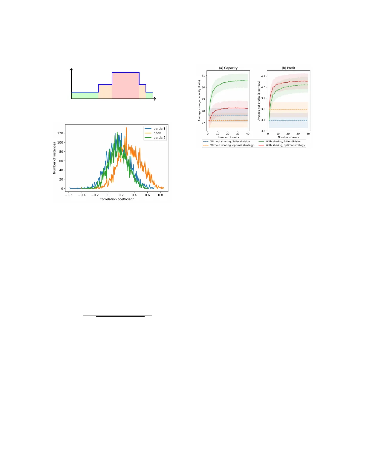
1 Optimal Electricity Storage Sharing Mechanism for Single Peaked T ime-of-Use Pricing Scheme Kui W ang, Y ang Y u, and Chenye W u Abstract —Sharing economy has disrupted many industries. W e for esee that electricity storage systems could be the enabler for sharing economy in electricity sector , though its implementation is a delicate task. Unlike in the 2- tier T ime-of-Use (T oU) pricing, where gr eedy arbitrage policy can achieve the maximal electricity bill savings, most existing T oU schemes consist of multiple tiers, which renders the arbitrage challenging . The difficulty comes from the hedging against multiple tiers and the coupling between the decisions across the day . In this work, we focus on designing the energy sharing mechanism for single peaked T oU scheme. T o solve the problem, we identify that it suffices to understand the arbitrage policies for two f orms of 3-tier T oU schemes. W e submit that under mild conditions, the sharing mechanism yields a unique equilibrium, which supports the maximal social welfare. Index T erms —Electricity storage, Time-of-Use pricing, op- timal control, sharing economy I . I N T RO D U C T I O N Sharing economy exploits huge Internet’ s value to heavy financial-cost yet idle assets [1]. This emer ging business model is already disrupti ve for large industries such as transportation, accommodation and micro finance [2]. W e notice that there are tremendous idle assets on the power grid, which already make the sharing economy business model attractiv e in electricity economics. How- ev er, the operational complexity due to physical con- straints leads to computational challenges in the sharing market design and operation for the idle assets. The current exploration on the sharing opportunities in electricity sector concentrates on real and virtual demand side assets. All relative studies demonstrate that such sharing opportunities need to be supported by three pil- lars: appropriate control policy with physical constraints, smart market design inducing incentive compatibility , and ef ficient algorithms to find the Pareto equilibrium. The authors are with the Institute for Interdisciplinary Information Sciences (IIIS), Tsinghua Uni versity , Beijing, China, 100084. C. W u is the correspondence author . Email: chenyewu@tsinghua.edu.cn. W e imagine the first adopters could be to share the electricity storage in behind-the-meter setting [3]. This is because the major concern in electricity sector comes from the regulatory uncertainty , and behind-the-meter setting is outside the purview of the utility . In such a setting, the firms could utilize their storage systems to arbitrage against the T oU pricing scheme, and share the excess energy via a local spot market. In essence, this opportunity requires each firm to better utilize the unused capacity in its storage system, which motiv ates us to design the electricity storage sharing mechanism. It still warrants significant efforts to bring sharing elec- tricity storage to practice. W u et al. propose a styl- ized model for storage sharing where in an industrial park, each firm faces 2-tier T oU pricing scheme [4]. This stylized model elegantly lays out the theoretical foundation for the sharing economy business model. W e further this result by generalizing from 2-tier to practical multi-tier T oU schemes. It is challenging e ven for a single firm’ s decision making, since it needs to hedge ag ainst multiple tiers and its decisions across the day are closely coupled together . The sharing market will emerge not only during peak but also partial peak periods. Hence, the market structure is more complex for examining the equilibrium beha vior . In this work, we try to understand the system beha vior (including indi vidual’ s decision making as well as the Nash equilibrium (N.E.) behavior in various sharing markets) in single peaked 1 T oU scheme. W e offer explicit formula to characterize the spot prices in the sharing markets. A. Related W ork Researchers ha ve designed control policies for dif ferent pricing schemes. W u and Y u proposed an optimal policy to arbitrage against 3-tier T oU pricing to maximize the arbitrage profits in [5]. For dynamic pricing, Qin et al. proposed an online modified greedy algorithm 1 Single peaked T oU scheme: Each day , the rate first increases from off peak to peak, and then decreases to next off peak period. 2 and proved its sub-optimality compared to offline [6]. V an de ven et al. proposed an optimal control policy for storage charging and discharging under Markovian random rates and demands [7]. T o the best of our knowledge, optimal control policy for general T oU has not been fully in vestigated. The literature on sharing economy in electricity sector emerges only recently , most of which inv estigated the cooperation of consumers to hedge against stochastic risks. For example, Zhao et al. introduced the optimal risky power contracts to the aggregation of multiple wind power plants for better bidding ag ainst 2-settlement markets in [8]. Bitar et al. explored the quantity risk sharing opportunities among wind po wer plants in nodal pricing scheme [9]. Chakraborty et al. introduced the rooftop PV sharing mechanism for active users in [10]. Perera et al. proposed a solar power sharing mechanism while a voiding the high v oltage impact to grid [11]. Zhao and Khazaei designed a cooperative game to aggregate multiple rene wable po wer plants and proved that the core supports the social welfare [12]. As for storage sharing, T ushar et al. proposed an auction- based storage sharing mechanism, where a unique equi- librium exists [13]. Chakraborty et al. cast the storage sharing problem in 2-tier T oU pricing as a coalitional game [14]. Different from previous works, we seek to design spot markets enabling the storage sharing, and offer the e xplicit characterization for the sharing prices. B. Our Contrib utions In this work, we significantly extend our pre vious works [4] and [5] by designing the optimal storage sharing mechanism for single peaked multi-tier T oU scheme to minimize all firms’ total cost for ener gy utilization. In the sharing mechanism, we analytically examine the sharing prices in spot markets, and each individual’ s optimal decision making to minimize its o wn cost. In summary , our principal contribution can be summarized as follows: • Optimal contr ol policy: W e propose the optimal control policy for standalone firm to arbitrage against single peaked T oU pricing scheme. Based on this control policy , we solve the individual optimal in vestment decision-making problem. • Sharing spot market: W e identify that sharing could happen in all non-off peak periods. For each period, we identify the aggregator-firms interaction game, and characterize its N.E.. The N.E. consists of the sharing prices and each indi vidual’ s decision making. W e also provide the sufficient conditions for the existence of N.E.. • P erformance assessment: W e prove that the out- come of our proposed sharing mechanism supports the maximal social welfare. W e use simulation to compare our sharing mechanism and alternativ es. The rest of the paper is organized as follows. Section II introduces the system model. Then, we propose the individual optimal control policy for arbitrage in Section III. Based on this control policy , we identify the market structure in Section IV. Then, Section V deriv es the optimal sharing mechanism for three-tier T oU scheme. Inspired by the intuition from Section V, we fully solve the problem for general single peaked T oU scheme in Section VI. Simulation verifies the performance of our proposed mechanism in Section VII. Section VIII gi ves concluding remarks and points out future work. W e pro vide all the necessary proofs in the Appendix. I I . S H A R I N G E L E C T R I C I T Y S T O R AG E Assume a single peaked multi-tier T oU is implemented in an industrial park, where firms can inv est storage for hedging against the price risks. T o simplify the analysis, we suppose that an aggregator in the park coordinates the storage sharing and energy management, such as procuring ener gy from the grid. T o obtain more insights through a stylized model, we make the following assumptions: 1) Arbitrage opportunity exists: the largest rate gap among hours is greater than the amortized cost of the storage in vestment. 2) All players are price takers of T oU prices. 3) All users’ hourly energy consumption is inelastic. 4) Demands in different periods are independent. 5) Ener gy loss in storage operation is ne gligible. 6) Firms make in vestment decisions simultaneously . Assumption 1 is already practical for many T oU pricing schemes thanks to the decreasing cost for storage sys- tems. For example, the amortized cost for T esla Po wer 2.0 Lithium-ion over its 10-year lifetime is only 14 ¢/kWh per day [15]. Assumption 2 implies that the user behaviors are not large enough to influence the T oU prices. This is reasonable for our industrial park setting. Howe ver , we want to emphasize that, when designing the sharing prices in our main results, we do consider all firms compete in the energy sharing market. Assumption 3 price demand X 1 X 2 off peak partial peak π ` π 1 π 2 (a) Ramp-up scheme price demand X 1 0 X 2 0 peak partial of f peak π ` π 2 0 π 1 0 (b) Ramp-down scheme Fig. 1: T wo basic 3-tier T oU pricing. 3 implies that without storage systems, all the firms have already fully e xploited their o wn flexibilities in response to T oU prices. This allo ws us to focus on the additional benefits brought by the storage systems and establish a stylized model. W e use numerical study to highlight that the performance of our scheme is close to that of the offline optimal with real data under assumption 4. The next assumption is temporary for more intuition during the analysis. W e drop this assumption in Appendix A for general conclusions. The last one is the common technical assumption for game theoretic analysis. I I I . O P T I M A L C O N T RO L F O R S TA N DA L O N E F I R M The firms make sharing decisions according to their energy consumption patterns and storage control. Thus, the storage sharing market design and arrangement must be built upon the understanding of individual’ s decision. The individual control polic y in 3-tier T oU scheme has been clarified by [5]. W e first summarize this result and then examine the individual storage control policy for a general single peaked T oU scheme. A. ( M , C ) Storage Contr ol P olicy for 3-tier T oU Scheme The analysis for 3-tier T oU scheme in [5] rev eals the nature of the storage control problems in the single peaked T oU schemes: there are two basic schemes of storage control sho wn in Fig. 1. The optimal control for ramp-down scheme (as sho wn in Fig. 1 (b)) is a greedy policy: fully charge the battery during the of f peak period and maximally use the stored energy sequentially from the peak to the partial peak period. The optimal storage control for ramp-up scheme (as shown in Fig. 1 (a)) is refereed to as the ( M , C ) control policy in [5], where C denotes the storage capacity and M denotes the energy reserv ed for peak demand use. Denote the random partial peak and peak demand by X 1 and X 2 , respectively . F X 2 ( · ) is the cumulativ e density Fig. 2: Single peaked T oU pricing scheme. function ( cdf ) of random v ariable X 2 ; F X 1 + X 2 | X 2 >M ∗ is the conditional cdf of X 1 + X 2 giv en X 2 > M ∗ ; π h , π m , π ` are the peak, partial peak and off peak rates, respectiv ely; π s is the amortized in vestment cost of storage. Then, the optimal parameters for ( M , C ) control policy can be determined as follo ws: M ∗ = F − 1 X 2  π h − π m π h − π `  , C ∗ = F − 1 X 1 + X 2 | X 2 >M ∗  π m − π ` − π s π m − π `  . (1) B. General Single P eaked T oU without Sharing Note that the ( M , C ) policy manifests that inserting a partial peak period sophisticates the storage control in two ways: introducing additional randomness to the capacity decision and additional decision problem of discharging strategy in partial peak period. In a general single peaked T oU scheme, there are more than one partial peak periods, which will significantly increase the complexity of the storage control problem. Figure 2 plots the general single peaked T oU scheme. The scheme consists of an of f peak period, followed by p ramp-up periods between off peak (denoted by RU j , j = 1 , · · · , p ) and peak, followed by q ramp-down periods between peak and off peak (including the peak, denoted by RD j , j = 1 , · · · , q ). R U j (RD j ) is also referred to as j th ( ( p + j ) th ) period of the day for brief statement. W e denote the electricity rate in off peak period by π ` ¢/kWh, and the rate in τ th period by π τ ¢/kWh. T o minimize each firm’ s electricity bill, the optimal decisions for storage inv estment and storage control depend on the distributions of firm’ s random demand in each period. W e denote firm i ’ s demand in τ th period by X i τ . In the subsequent analysis for standalone firm’ s decision making, when there is no confusion, we will drop the superscript i for con venience. 4 W e follow the ( M , C ) type control policy for general single peaked T oU pricing. Specifically , the control pol- icy for a firm can be decomposed as follo ws: • In vestment Decision: T o minimize its electricity cost, the firm will in vest C kWh of storage. • Initialization in Off P eak: Each day , the firm will fully char ge the storage system during of f peak. • Operation in R Us: In RU j , use the energy in the storage while reserving at least M j for future use. • Operation in RDs: In RD j , use the energy in the storage as much as possible, purchase the unmet demand from the grid. For the j th ramp-up period R U j , we define a function M R j ( M j ) as the marginal rev enue for reserving M j . Specifically , M R j ( M j ) = p + q X k = j +1 ( π k − π ` ) P k j ( M j , M ∗ j +1 , · · · , M ∗ p ) , (2) where P k j ( M j , M ∗ j + 1 , · · · , M ∗ p ) is the probability that since R U j , k th ( k > j ) period is the first time that the firm needs to purchase electricity from the grid, giv en optimal reservations for following periods M ∗ j +1 , · · · , M ∗ p . The marginal re venue measures the expected additional profit that one more unit energy reservation may bring to the firm. This one more unit reservation brings profit exactly at the first time that the firm needs to purchase energy from the grid, which is the economic intuition of Eq. (2). In order to guarantee the uniqueness of optimal reservation, we make the following technical assumption: Assumption 7 : For each firm’ s demand in each non off peak period (denoted by X ), its probability density function f X ( x ) is differentiable, and f X ( x ) > 0 if x ≥ 0 . W ith this assumption, we can show: Lemma 3.1: If Assumption 7 is satisfied, then M R j ( M j ) is monotone and the optimal reservation is unique. The optimal control polic y in RU j balances the opportu- nity costs of energy purchasing at current time slot and the expected marginal re venue of reserving for future at the crossing point: π j − π ` = M R j ( M ∗ j ) . (3) The associated optimal in vestment is the capacity C ∗ balancing the amortized fixed cost and the marginal benefit of in vestment: π s = X p + q k =1 ( π k − π ` ) P k 0 ( C ∗ , M ∗ 1 , · · · , M ∗ p ) , (4) where P k 0 ( C, M ∗ 1 , · · · , M ∗ p ) is the probability that since the off peak, k th period is the first time that the firm need purchase electricity from the grid, giv en storage in vestment C and the optimal reserv ations M ∗ 1 , · · · , M ∗ p . The above policy builds the foundation for analyzing storage sharing market. It is used to calculate the social optimal strategy benchmarking the efficienc y of the shar- ing mechanism, and to examine the firm’ s strategy in the sharing economy . Note that in both R U and RD periods, the optimal storage control action for each individual firm is to discharge the storage (while reserving certain energy during R U periods). This greedy control action will change dramatically when sharing is allo wed. I V . S T O R AG E S H A R I N G A N D I N V E S T M E N T It warrants designing a sequence of mechanisms to coordinate firms’ price-arbitrage decisions. Those mech- anisms respecti vely induce an aggre gated in vestment decision and a set of storage sharing market. W e assume that an aggregator coordinates the sharing market. W e want to emphasize that in our subsequent game theoretic analysis, we do not make price taker assumption. In fact, we explicitly consider firm’ s competition, which leads to the ef ficient sharing price. T wo coupled games respectiv ely arrange the mechanism of the storage in vestment and the associated storage sharing rules. The firms first collectiv ely determine the storage capacity according to their cumulativ e net benefit from the storage utilization. Then, the firms interact with the aggregator for sharing the storage to arbitrage against the T oU price in each period. Next, we se verally describe the tw o games. A. Aggr egator -F irm Inter action Game The sharing market can be formulated as a Stackelberg game economically enabling energy trading between the firms. In this game, a non-for-profit aggregator pursues for minimizing the total electricity cost in the industrial park. The aggregator acts as the game leader and an- nounces the sharing price in ev ery period while the firms respond to the price as follo wers. Thus, we can formally define the Aggre gator-Firm Interaction Game (AFIG) as follows: Aggr e gator-F irm Interaction Game (AFIG) 5 Players: The aggregator is the leader , and the firms are the follo wers. Strate gy Spaces: The aggregator sets the sharing prices π a τ ∈ R + at each period τ , τ = 1 , · · · , p + q ; the firms respond to the prices by deciding their energy procurement or supply D i τ ∈ R , τ = 1 , · · · , p + q (positiv e D i τ implies energy procurement for firm i at period τ while negati ve D i τ implies energy supply to the sharing market). Utilities: The non-for-profit aggregator seeks to mini- mize the total energy cost in the industrial park with its own budget balance guaranteed, while each firm seeks to minimize its o wn electricity bill. T o better characterize each firm’ s utility function, we formulate the following optimization problem for each firm i : min D i 1 , ··· ,D i p + q J i τ ( D i 1 , · · · , D i p + q | π a 1 , · · · , π a p + q ) = E n X p + q j =1 π a j D i j o | {z } cost in non off peak periods + π ` E { D i 0 } | {z } recharge during off peak , (5) The D i τ ’ s are used to meet firm i ’ s demand at each period τ and simultaneously guarantee the storage temporal constraints. W e choose not to explicitly write out the constraints, since we hav e deriv ed the optimal ( M , C ) policy for single firm. The aggregator can simple seek to set π a 1 , · · · , π a p + q , such that the firms’ aggre gate behavior follows the optimal ( M , C ) polic y . Note that, in AFIG, we assume that the firms have already purchased certain amount capacity of storage systems, i.e., C 1 , · · · , C n . Hence, the equilibrium prices π a 1 , · · · , π a p + q are dependent on the storage capacities. Next, we introduce the Capacity Decision Game for firms to make the optimal storage in vestment decision for itself. B. Capacity Decision Game In the Capacity Decision Game (CDG), the firms com- pete for storage in vestment. Each firm’ s decision bal- ances between in vesting more capacity at the be ginning and exposing to more risks in the future. The profit of in vesting more storage comes from: the higher cost saving due to av oiding the energy procurement during the high-price periods as well as the larger profit from Fig. 3: The coupling between two games: CDG and AFIG. selling the energy stored in the storage. W e formally introduce the CDG as follo ws: Capacity Decision Game (CDG) Players: All the firms in the industrial park. Strate gy Spaces: Storage in vestment decision C i ∈ R + for each firm i . Utility: Each firm seeks to minimize its expected daily cost I i , i.e., min C i I i ( C i , C − i ) = π s C i | {z } in vest cost + X p + q j =1 E { π a j D i j } | {z } cost in non off peak periods + π ` E { D i 0 } . | {z } recharge cost (6) Here, C − i = P j 6 = i C j refers to the sum of all other firms’ capacities. More precisely , note that π a j ’ s are determined by C i and C − i , which naturally leads to the game formulation. D i j and D i 0 are actually related to C i . Remark: The outcome of CDG heavily depends on the aggregator’ s pricing scheme in AFIG. This is how the two games are coupled together . W e visualize the coupling in Fig. 3 from two perspecti ves: the time sequence and the analytical sequence. Specifically , in the timeline, the firms first determine the capacity (the decision of CDG), and then the aggregator arranges the AFIG each day . Howe ver , to analyze the optimal decisions to the two games, we need to solve them in backward. W e first analyze the N.E. (especially the aggregator’ s sharing prices) in the AFIG, and then, based on this information, we can understand the optimal storage in vestment decision for each firm in the CDG. T o ease the understanding of the sequential decision making, we first analyze the coupling dynamics through simple cases (three-tier T oU) and then generalize the 6 results to general single peak ed T oU. V . M A R K E T A NA LY S I S F O R T H R E E - T I E R T O U This section discusses the firms’ strategies and mar- ket equilibria in the three-tier T oU, which rev eals the intuition of our proposed pricing mechanism, and the corresponding firm strategies as well as associated sys- tem impacts. There are two basic scenarios: the ramp- up scheme (R US) and the ramp-down scheme (RDS). W e separately discuss these two basic scenarios. W e first notice that the following two facts are true in both the R US and RDS. F act 1: Firms’ optimal strategy in the off-peak period is to fully rechar ge the storage without sharing their ener gy . F act 2: Firms only reserv e energy during R U periods. These two facts allo w us to narrow our focus on the firms’ strategies during the peak and partial peak periods, and their associated market dynamics. A. Ramp-Down Scheme In the RDS (as sho wn in Fig. 1 (b)), we model firm i ’ s peak (partial peak) demand as random variable X i 1 0 ( X i 2 0 ), and define the total demand during peak and partial peak periods by X c 1 0 and X c 2 0 , i.e., X c 1 0 = X i X i 1 0 ; X c 2 0 = X i X i 2 0 . Observing a greedy type polic y is optimal, the follo w f act dictates the N.E. during the partial peak period when the i th firm has u i units of electricity in the storage at the beginning of partial peak period and has to consume x i 2 0 units of electricity (the realization of X i 2 0 ) in the partial peak period. F act 3: The optimal electricity sharing price for maximal social welf are in partial peak should be set as π a ∗ partial =  π 2 0 , if x c 2 0 ≥ u c , π ` , if x c 2 0 < u c , (7) where x c 2 0 = P i x i 2 0 , denoted the realization of X c 2 0 ; and u c = P i u i . This fact is simply the result of competition among firms in dif ferent market conditions. In peak period, we propose the optimal pricing strategy for the aggregator to minimize the total cost of all firms when the realized demand is x i 1 0 for firm i : Mechanism 1: The optimal electricity sharing price in peak period of the aggre gator π a ∗ peak should be set as: π a ∗ peak =  π 1 0 , if x c 1 0 > C c , π 0 , if x c 1 0 < C c , where π 0 = π ` + ( π 2 0 − π ` ) Pr ( x c 2 0 > C c − x c 1 0 ) , x c 1 0 = P i ∈N x i 1 0 and C c = P i C i . The mechanism is deriv ed from the aggregator’ s system- cost minimization problem thus guarantees the optimal market equilibrium for social welfare, yielding the fol- lowing lemma: Lemma 5.1: The aggregator adopts pricing scheme in Mechanism 1 will lead the firms to make storage op- erations which supports social welfare (in terms of minimizing the total cost), while achiev es aggregator’ s budget balance (i.e., zero cost for the aggregator). • When the total realized demand exceeds the total amount of stored energy ( x c 1 0 > C c ), each firm will choose to greedily use up its storage since its own cost monotonically increases with its reservation u i : ∂ J i ∂ u i = π 1 0 − π ` − ( π 2 0 − π ` ) Pr ( x c 2 0 > u c ) > π 1 0 − π 2 0 > 0 . (8) • When the stored energy is suf ficient to satisfy realized the demand ( x c 1 0 < C c ), we have π a ∗ peak = π ` + ( π 2 0 − π ` ) Pr ( x c 2 0 > C c − x c 1 0 ) = E { π a ∗ partial | x c 1 0 } . (9) This yields that the first order optimality condition automatically holds: ∂ J i ∂ u i = π a ∗ peak − E { π a ∗ partial | x c 1 0 } = 0 . (10) That is, the firms hav e no incentiv e to make any en- ergy reservation in this case. T ogether with Eq. (8), Mechanism 1 indeed leads to the optimal greedy policy . The firms’ total expected profit from owning the stor- age, which is framed by the mechanism organizing the sharing mark et, shapes their storage-in vestment decisions in the CDG. Each firm balances the cost and benefit from owning the storage by minimizing the total cost I i ( C i , C − i ) , including the in vestment cost and the total expected cost from purchasing electricity . I i ( C i ,C − i ) = π s C i + E { π a ∗ peak D i peak } + E { π a ∗ partial D i partial } + π ` E { D i of f } , (11) 7 where C − i = { C j | j 6 = i } implicitly influences the shar - ing prices in peak and partial peak periods, and D i peak , D i partial and D i of f are firm i ’ s electricity deficit during the peak, partial peak and off peak period respecti vely . The N.E. of the CDG is summarized in the following theorem. Theor em 5.2: If CDG admits a N.E., then it is unique and can be characterized by C ∗ i = λ 1 E [ X i 1 0 | X c 1 0 = C ∗ c ] + λ 2 E [ X i 1 0 + X i 2 0 | X c 1 0 + X c 2 0 = C ∗ c ] , ∀ i, (12) where λ 1 = ( π 1 0 − π 2 0 ) f X c 1 0 ( C ∗ c ) ( π 1 0 − π 2 0 ) f X c 1 0 ( C ∗ c ) + ( π 2 0 − π ` ) f X c 1 0 + X c 2 0 ( C ∗ c ) , λ 2 = ( π 2 0 − π ` ) f X c 1 0 + X c 2 0 ( C ∗ c ) ( π 1 0 − π 2 0 ) f X c 1 0 ( C ∗ c ) + ( π 2 0 − π ` ) f X c 1 0 + X c 2 0 ( C ∗ c ) , and C ∗ c is the unique solution to Eq. (13) π s = ( π 1 0 − π ` ) Pr ( X c 1 0 > C c ) + ( π 2 0 − π ` ) Pr ( X c 1 0 < C c , X c 1 0 + X c 2 0 > C c ) . (13) Howe ver , CDG may not always admit a N.E. in that the cost function I i ( C i , C − i ) could be non-con ve x with respect to C i . W e need the following technical alignment conditions to guarantee the e xistence of the N.E.: Theor em 5.3: If the follo wing two conditions hold: ∂ E [ X i 1 0 | X c 1 0 = r ] ∂ r ≥ 0 , ∀ i, (14) ∂ E [ X i 1 0 + X i 2 0 | X c 1 0 + X c 2 0 = c ] ∂ c ≥ 0 , ∀ i, (15) then CDG for RDS al ways admits a unique N.E.. Remark: The two technical alignment conditions merely require on expectation , the energy consumption for each individual firm should align with the trend of total load. This can be guaranteed by checking the pairwise correlations. Intuitiv ely speaking, as long as there is only a small portion of negativ e pairwise correlations, the alignment conditions automatically hold. W e hav e observed the distrib ution of correlation for the residential loads under the SCE Grandfathered Rate Plans [16]. The residential loads in Austin from Pecan street [17], only produce 2 . 3% neg ativ e pairwise correlations in peak period and 2 . 0% for the total demands in peak and the following partial peak periods. The abov e analysis presents how firms’ demands and T oU designs determine sharing market design as well as the storage in vestment. B. Ramp-Up Scheme (R US) In contrast to the greedy strategy in RDS, the firms ha ve an extra choice that is to reserve electricity for future in addition to sharing. Since the analysis is almost identical, we will only present necessary intuition for the analysis in R US. W e denote firm i ’ s random partial peak and peak demand by X i 1 and X i 2 , respectiv ely , and denote its realized partial and peak demand by x i 1 and x i 2 . Mechanism 2: The optimal pricing scheme for the ag- gregator in RUS is to set π a peak and π a partial as follows: π a ∗ peak =  π 2 , if x c 2 > u c , π ` , if x c 2 < u c , (16) π a ∗ partial =  π 1 , if x c 1 > C c − M , π 00 , if x c 1 < C c − M , (17) where x c 2 = P i x i 2 , u c = P i u i and π 00 = π ` + ( π 2 − π ` ) Pr ( X c 2 > C c − x c 1 ) , and M = F − 1 X c 2  π 2 − π 1 π 2 − π `  . (18) W e can show the optimality of Mechanism 2 through the following lemma: Lemma 5.4: The aggregator adopts pricing scheme in Mechanism 2 will lead the firms to make storage op- erations which supports social welfare (in terms of minimizing the total cost), while achiev es aggregator’ s budget balance (i.e., zero cost for the aggregator). W e would also like to point out that in R US, there exists another CDG and this time the technical alignment condition to guarantee the existence of N.E. is different: Theor em 5.5: If for each firm i , ∂ E [ X i 1 + X i 2 | X c 1 + X c 2 = r, X c 1 < r − M ] ∂ r ≥ 0 , (19) Then, the CDG for R US admits a unique N.E.. Remark: Again, this technical alignment condition is not hard to meet. It also requires on expectation , the energy consumption for each indi vidual firm should align with the trend of total load. 8 V I . G E N E R A L S I N G L E P E A K E D T O U S C E NA R I O Having the intuition from analyzing three-tier T oU schemes, we know that the whole decision process couples with two games: AFIG and CDG. In this section, we analyze the sharing mechanism for single peaked T oU scheme. Again, the firms will follow the agggre- gator’ s price signal to make their sharing decisions to minimize their own cost in the non off peak periods, and make storage sizing decisions according to CDG’ s N.E.. Howe ver , the temporal coupling brings huge dif ficulties. For τ th non off peak period, u c τ − 1 refers to the total energy left in the storage at the beginning of the period; x c τ refers to the realized total demand in the period; P k τ ( x c τ , u c τ − 1 ) refers to the probability that since τ th non off peak period, k th period ( k > τ ) is the first time that the collectiv e need purchase electricity from grid, based on the realized demand x c τ and the initial reservation u c τ − 1 . Based on these quantities, we can use the same intuition of Eq. (2) to obtain the expected marginal profit for reserving energy at each time slot. On the other hand, the marginal cost for reserving ener gy at time τ is simply π a τ , the sharing price that the energy set in τ th period. And we seek to design the optimal prices ( π a ∗ τ ’ s) of the aggregator . For j th non off peak period, j = p + q , · · · , 1 , we propose that the sharing price π a j should satisfy π a ∗ j = π ` + p + q X k = j ( π k − π ` ) P k j ( x c j , u c j − 1 ) . (20) Notice that if realized demand ( x c j ) is more than total energy left ( u c j − 1 ), then the collectiv e need purchase electricity from grid in period this period; i.e., P j j = 1 , yielding π a ∗ j = π j , which coincides with intuition. This sharing mechanism leads to another CDG: if the game admits a N.E., it is unique and gi ven by C ∗ i = q X l =1 ρ l ( C ∗ c ) E " p + l X k =1 X i k      p + l X k =1 X c k = C ∗ c , n X k =1 X c k < C ∗ c − M ∗ n , 1 ≤ n ≤ p # , (21) where ρ l ( C ∗ c ) = ( π p + l − π p + l +1 ) f { P p + l k =1 X c k } ( C ∗ c ) P q m =1 ( π p + m − π p + m +1 ) f { P p + m k =1 X c k } ( C ∗ c ) , and C ∗ c is the unique solution of π s = X p + q k =1 ( π k − π ` ) P k 0 ( C c ) , (22) where π p + q +1 = π ` , P k 0 ( C c ) refers to the probability of that since off peak, k th non off peak period is the first time that the collectiv e need purchase electricity grid, based on in vestment C c . T o ensure the existence of N.E., we need the follo wing technical alignment conditions: Theor em 6.1: If ∀ RD j , j : 1 ≤ j ≤ q , ∂ G i j ( r ) ∂ r ≥ 0 , ∀ i (23) where G i j ( r ) = E " p + j X k =1 X i k      p + j X k =1 X c k = r , n X k =1 X c k < r − M ∗ n , 1 ≤ n ≤ p # , then the N.E. of CDG in the single peaked multi-tier T oU pricing exists. Remark: The N.E. ’ s of AFIG and CDG support social welfare for all firms. By the definition of equilibrium, they can automatically ensure individual rationality . In fact, the y enjoy additional properties, as summarized in the follo wing proposition: Pr oposition 6.2: The equilibria of the sharing markets and CDG in single peaked multi-tier T oU pricing scheme enjoy the following properties: (a) Coalitional stability : No subset of firms are better off by defecting to form their own coalition. (b) No pure-str ate gy play : If firm i has no demand in all periods other than the off peak, it will not inv est in storage. Hence, the aggregator can be in a neutral position to coordinate the mark et. V I I . S I M U L A T I O N S T U D I E S T o ev aluate the performance of our control policy and sharing mechanism, we use real household profiles (in summer of 2016) from Austin in Pecan Street [17]. W e compare our control policy with a simple policy where the decisions for all the firms across the day are decoupled. That is, the firms won’ t reserve energy for future use. They will focus on the arbitrage (and sharing) opportunities between off peak period and other periods. In a single peaked pricing scheme with k periods, this simple policy is the same as solving k − 1 2-tier (one 9 price 13¢ 28¢ 52¢ 0AM 8AM 2PM 8PM 10PM12PM Fig. 4: SCE Grandfathered Rate Plans T oU-D-A [16]. Fig. 5: Diversity of partial peak and peak demands. non off peak and off peak) storage sharing problems. W e refer to this simple policy as “2-tier di vision”. W e use a real 3-tier T oU pricing scheme as shown in Fig. 4 for simulation. W e use T esla Po wer 2.0 Lithium- ion to estimate π s : amortized over 10-year lifetime, the T esla battery costs 14 ¢/kWh per day [15]. Pairwise correlation coefficient reflects the sharing mar- ket conditions. The pairwise correlation coefficient be- tween the consumptions of firm a and firm b in j th period can be calculated as follo ws: ρ ab j = E { X a j X b j } − E { X a j } E { X b j } q V ar { X a j } · V ar { X b j } . (24) If most coefficients are around 1, then there will be little room for sharing. Figure 5 plots the histogram of the pairwise correlation coefficients of the real demands in dif ferent periods. W e can observe that the mean coefficient is around 0.16 while only 7% of coefficients exceed 0 . 5 . This illustrates certain room for sharing markets in practice. Figure 6 compares the different control policies. Our proposed sharing mechanism achiev es about 7 ¢/day more profit compared with 2-tier di vision and about 23 ¢/day more profit compared with no sharing scenario. If the industrial park owner strategically selects the firms with more div ersified load profiles, our sharing Fig. 6: Capacity and profit for different mechanisms. The shaded regions in Fig. 6 reflects the interval between mean-var/20 and mean+var/20 over dif ferent community size. mechanism can yield more profits. W e highlight the impact of independent demand assump- tion is not too restricti ve in Fig. 7. The offline optimal denotes the storage operation with all the future demand information, which yields 33 . 0% average cost saving compared to the benchmark when there is no storage in the system at all. Our proposed optimal storage sharing mechanism achiev es 30 . 4% expected cost saving. The 2 . 6% difference is the aggregate effects of unknown future information and the independent demand assump- tion. V I I I . C O N C L U S I O N S A N D F U T U R E W O R K W e propose a sharing mechanism for electricity storage for single peaked T oU pricing scheme. W e show that this sharing mechanism supports the maximal social welfare. W e are interested in understanding the sharing mecha- nism for the dynamic pricing schemes. The uncertainties in the electricity rates will incur challenge for theoretical analysis. It will be also interesting to consider the sharing market where the firms make their decisions sequentially instead of simultaneously . This scenario reflects the dynamics of firm’ s joining the industrial park. R E F E R E N C E S [1] J. J. Horton and R. J. Zeckhauser, “Owning, using and renting: Some simple economics of the “sharing economy”, ” National Bureau of Economic Research, T ech. Rep., 2016. [2] PwC analysis. (2017) Projected growth rate of sharing economy and traditional rental worldwide between 2013 and 2025. [Online]. A vailable: http://alturl.com/n9yug 10 Fig. 7: Cost comparison between different kinds of storage utilization. [3] D. Kalathil, C. W u, K. Poolla, and P . V araiya, “The sharing economy for the electricity storage, ” IEEE T rans. on Smart Grid , pp. 1–1, 2018. [4] C. Wu, D. Kalathil, K. Poolla, and P . V araiya, “Sharing electricity storage, ” in Pr oc. of IEEE CDC . IEEE, 2016, pp. 813–820. [5] C. Wu and Y . Y u, “Optimal control for electricity storage against three-tier tou pricing, ” in Proc. of IEEE APSIP A ASC . IEEE, 2018, pp. 737–741. [6] J. Qin, Y . Chow , J. Y ang, and R. Rajagopal, “Online modified greedy algorithm for storage control under uncertainty , ” IEEE T rans. P ower Syst. , vol. 31, no. 3, pp. 1729–1743, 2016. [7] P . M. van de V en, N. Hegde, L. Massouli ´ e, and T . Salonidis, “Optimal control of end-user energy storage, ” IEEE T rans. on Smart Grid , vol. 4, no. 2, pp. 789–797, June 2013. [8] Y . Zhao, J. Qin, R. Rajagopal, A. Goldsmith, and H. V . Poor, “W ind aggregation via risky power markets, ” IEEE T rans. P ower Syst. , vol. 30, no. 3, pp. 1571–1581, May 2015. [9] E. Y . Bitar, E. Baeyens, P . P . Khargonekar , K. Poolla, and P . V araiya, “Optimal sharing of quantity risk for a coalition of wind power producers facing nodal prices, ” in Pr oc. of IEEE ACC . IEEE, 2012, pp. 4438–4445. [10] P . Chakraborty , E. Bae yens, P . P . Khargonekar , K. Poolla, and P . V araiya, “ Analysis of solar energy aggregation under various billing mechanisms, ” IEEE T rans. on Smart Grid , 2018. [11] B. K. Perera, P . Ciufo, and S. Perera, “Po wer sharing among multiple solar photov oltaic (pv) systems in a radial distribution feeder , ” in Proc. of IEEE AUPEC . IEEE, 2013, pp. 1–6. [12] Y . Zhao and H. Khazaei, “ An incentiv e compatible profit alloca- tion mechanism for renewable energy aggregation, ” in Proc. of IEEE PESGM , July 2016, pp. 1–5. [13] W . Tushar , B. Chai, C. Y uen, S. Huang, D. B. Smith, H. V . Poor , and Z. Y ang, “Energy storage sharing in smart grid: A modified auction-based approach, ” IEEE T rans. on Smart Grid , vol. 7, no. 3, pp. 1462–1475, May 2016. [14] P . Chakraborty , E. Bae yens, K. Poolla, P . P . Khargonekar , and P . V araiya, “Sharing storage in a smart grid: A coalitional game approach, ” IEEE T rans. on Smart Grid , 2018. [15] Powerwall, tesla. [Online]. A vailable: http://alturl.com/hkgir [16] SCE Grandfathered Rate Plans: TOU-D-A. [Online]. A vailable: http://alturl.com/66iyu [17] Pecan street. [Online]. A vailable: http://alturl.com/zjqk2 A P P E N D I X A. Assumption 5 Relaxation The imperfect charging efficienc y and discharging ef- ficiency will heavily affect the storage sharing mech- anism characterization. Denote the charging efficienc y by η i and the discharging efficienc y by η o . Below , we show how to characterize the ( M , C ) control policy , the sharing price π a j ’ s, the optimal storage in vestment c ∗ i for each firm i , and the technical alignment conditions, all in terms of η i and η o . W ith the charging and discharging ef ficiency , The opti- mal collectiv e reserv ation in j th non off peak period M j can be formulated as: π j η o − π ` /η i = p + q X k = j +1 ( π k η o − π ` /η i ) P k j ( M j , M ∗ j +1 , · ·· , M ∗ p ) . (25) For j th non of f peak period, j = p + q , · · · , 1 , the sharing price π a j should satisfy π a ∗ j η o = π ` /η i + p + q X k = j ( π k η o − π ` /η i ) P k j ( x c j , u c j − 1 ) . (26) This sharing mechanism again leads to a CDG: if the game admits a N.E., it is unique and gi ven by C ∗ i = q X l =1 ρ l ( C ∗ c ) E " p + l X k =1 X i k      p + l X k =1 X c k = C ∗ c η o , n X k =1 X c k < ( C ∗ c − M ∗ n ) η o , 1 ≤ n ≤ p # , (27) where ρ l ( C ∗ c ) = ( π p + l − π p + l +1 ) f { P p + l k =1 X c k } ( C ∗ c η o ) P q m =1 ( π p + m − π p + m +1 ) f { P p + m k =1 X c k } ( C ∗ c η o ) , and C ∗ c is the unique solution of π s η o = X p + q k =1 ( π k η o − π ` /η i ) P k 0 ( C c ) , (28) 11 where π p + q +1 = π ` / ( η i η o ) , P k 0 ( C c ) refers to the proba- bility of that since off peak, k th non of f peak period is the first time that the collective need purchase electricity grid, based on in vestment C c . T o ensure the e xistence of N.E., we need the following technical alignment conditions: Pr oposition A.1: If ∀ RD j , j : 1 ≤ j ≤ q , ∂ G i j ( r ) ∂ r ≥ 0 , ∀ i (29) where G i j ( r ) = E " p + j X k =1 X i k      p + j X k =1 X c k = r η o , n X k =1 X c k < ( r − M ∗ n ) η o , 1 ≤ n ≤ p # , then the N.E. of CDG in the single peaked multi-tier T oU price exists. B. Optimality of the Contr ol P olicy Remark: W e only prov e those results for the general single peaked T oU in the following parts. Results for the two basic 3-tier T oU schemes are special cases of the general scenario and we only use them to obtain more intuitions in the main content. In this subsection, we sho w that the arbitrage control policy proposed in Section III-B can bring maximal profit using backward induction. Firstly , we prove that the greedy policy is optimal in RD periods. Secondly , we prov e that the threshold policy is optimal in R U periods and characterizes the best thresholds at the same time. Finally , we characterize the optimal inv estment decision. For j th non off peak period of the day , we denote energy left in the storage at the be ginning by u j − 1 , and ener gy left in the storage at the end by u j , the electricity we need to purchase by D j and the realized demand in this period as x j . Let D 0 be the electricity amount we need to purchase in of f peak for recharge. Greedy P olicy in RD Periods Is Optimal W e first examine the tri vial case in RD q , the last non off peak period. It is straightforw ard to see that the optimal strategy is to discharge the storage as much as possible, which constructs our induction basis. Now we prov e the optimality for the rest RD periods . Assume that greedy policy is optimal from RD q to RD j +1 . W ith this hypothesis, we want to sho w that greedy polic y is optimal in RD j . The total cost J p + j in RD j and follo wing RD periods is as follows: J p + j ( u p + j ) = π p + j ( u p + j + x p + j − u p + j − 1 ) | {z } buy deficit in RD j + p + q X k = p + j +1 π k E { D k } | {z } buy deficit in following RDs + π ` E { D 0 } | {z } recharge cost . (30) Examining J p + j ’ s first order deri v ativ e with respect to u p + j , we can conclude that ∂ J p + j ∂ u p + j > 0 , (31) which means the greedy polic y is optimal in RD j . By now we complete our proofs for all RD periods, we focus on the R U periods in the subsequent analysis. Threshold P olicy in R U periods The induction basis is to examine the threshold policy for R U p is optimal. This is a special case of the ( M , C ) policy in [5]. Based on this induction basis, we can use backward induction to complete our proof. T o guarantee the optimal reservation is unique in the ramp-up peri- ods, we need the deriv ativ e the total cost J j in RU j and following periods with respect to u j is monotone increasing, therefore we make the following technical assumption. Assumption 7 : For each firm’ s demand in each non off peak period (denoted as X ), its probability density function f X ( x ) is differentiable, and f X ( x ) > 0 if x ≥ 0 ; In vestment decision W e can regard the in vestment decision as a reserv ation decision in the virtual period R U 0 (off peak) with the rate π 0 = π s + π ` , then we get the optimal size C ∗ which satisfies Eq. (4). By now we hav e proved our control policy achiev es maximal profit.  C. Characterize N.E. of CDG In this subsection we characterize the N.E. of the CDG, and prove it supports maximal social welfare. Before we start, we define some useful functions for subsequent 12 analysis. δ ( C c ) = q X m =1 ( π p + m − π p + m +1 ) f { P p + m k =1 X c k } ( C c ) , γ i ( C c ) = q X j =1 ρ j ( C c ) E " p + j X k =1 X i k      p + j X k =1 X c k = C c , n X k =1 X c k < C c − M ∗ n , 1 ≤ n ≤ p # , and ρ l ( C c ) = ( π p + l − π p + l +1 ) f { P p + l k =1 X c k } ( C c ) P q m =1 ( π p + m − π p + m +1 ) f { P p + m k =1 X c k } ( C c ) . Giv en other firms’ in vestment decision C − i , firm i ’ s optimal in vestment decision can be stated as: C ∗ i = arg min C i I i ( C i , C − i ) . (32) I i is the total electricity cost of firm i . I i ( C i , C − i ) = π s C i | {z } in vest cost + X p + q j =1 E { π a ∗ j D i j } | {z } cost in non off peak periods + π ` E { D i 0 } . | {z } recharge cost (33) where D i j is the deficit of firm i in k th non off peak period, and D i 0 is the amount of ener gy that firm i needs to recharge its storage. Negati ve value means the firm shares its energy to others and obtain certain profit. Due to our pricing mechanisms, single firm’ s concrete reservations at N.E. in each non of f peak period do not influence its profit as we analyzed in Section IV -A. Thus, without loss of generality , we suppose firm i has zero reservation in each non off peak period. Then D i 1 = x i 1 − C i , D i j = x i j , j = 2 , · · · , p + q , D i 0 = C i . The deri vati ve of I i with respect to C i is ∂ I i ∂ C i = π s − p + q X k =1 ( π k − π ` ) P k 0 ( C c ) − δ ( C c )( γ i ( C c ) − C i ) . (34) Define α = π s − p + q X k =1 ( π k − π ` ) P k 0 ( C ∗ c ) , (35) β = δ ( C ∗ c ) . (36) Note that Assumption 7 guarantees that β > 0 and C ∗ > 0 , ∀ i . The definition of N.E. guarantees that for each firm i , its cost reaches minimum at C ∗ i : ∂ I i ∂ C i     C i = C ∗ i = α − β ( γ i ( C ∗ c ) − C ∗ i ) = 0 . (37) Summing o ver all firms yields nα − β ( X i γ i ( C ∗ c ) − C ∗ c ) = 0 , (38) where n is the number of firms. Note that P i γ i ( C ∗ c ) = C ∗ c , we can conclude that α = 0 . (39) Hence, Eq. (34) dictates that for each firm i , C ∗ i = γ i ( C ∗ c ) . (40) This implies C ∗ c satisfying Eq. (22), the optimal in vest- ment for the collectiv e, in other words, the firms make in vestment decisions which are optimal for the collectiv e in the N.E..  D. Alignment Conditions for the Existence of N.E. W e consider firm i ’ s decision C i when fixing the deci- sions of all other firms C ∗ − i as C ∗ k = γ k ( C ∗ c ) , k 6 = i. Define ν = X k 6 = i C ∗ k . According to (34), the deriv ativ e of expected daily cost of firm i with respect to C i is ∂ I i ∂ C i = π s − p + q X k =1 ( π k − π ` ) P k 0 ( C i + ν ) | {z } φ ( C i ) − δ ( C i + ν ) ( γ i ( C i + ν ) − C i ) | {z } ψ ( C i ) . (41) W e obtain φ ( C i ) is strictly monotone increasing with respect to C i in that ∂ 2 φ ( C i ) ∂ C 2 i = ( π p + q − ` ) θ 0 ( C i + ν ) > 0 , (42) where θ 0 ( C i + ν ) = 13 Z C i + ν − M ∗ 1 0 f X 1 ( x 1 ) · · · Z C i + ν − p − 1 P k =1 x k − M ∗ p 0 f X p ( x p ) f { P q k =1 X p + k } ( C i + ν − p X k = j +1 x k ) dx p · · · dx 1 > 0 . Here we use Assumption 7 once more. T o verify the monotonicity of ψ ( C i ) , we make critical use of the technical alignment conditions in (23) to conclude 1 = X k ∂ G k j ( r ) ∂ r | {z } ≥ 0 = ⇒ ∂ G i j ( r ) ∂ r ≤ 1 . And notice that p X j =1 ρ j ( C i + ν ) = 1 . It then follows that ∂ ψ ( C i ) ∂ C i = p X j =1 ρ j ( C i + ν ) ∂ G i j ( C i + ν ) ∂ ( C i + ν ) − 1 ≤ 0 . This means ψ ( C i ) is monotonically decreasing with respect to C i . W e obtain φ ( C i ) is strictly monotone increasing with respect to C i and ψ ( C i ) is monotone decreasing, so I i ( C i ) is strictly monotone increasing according to (41). Notice φ ( C ∗ i ) = ψ ( C ∗ i ) = 0 . As a result, we ha ve ∂ I i ∂ C i    < 0 C i < C ∗ i , = 0 C i = C ∗ i , > 0 C i > C ∗ i . This prov es that C ∗ i is the global minimizer of firm i ’ s cost, establishing that ( C ∗ 1 , c ∗ 2 , · · · , C ∗ n ) is the unique N.E..  E. Pr oof of Pr oposition 6.2 (a) Coalitional Stability For firms { 1 , 2 , ..., n } , we form coalitions A j ⊂ { 1 , ..., n } such that A i ∩ A j = ∅ , [ k A k = { 1 , ..., n } . The initial CDG G induces a new CDG H with players A i and associated cost I A i = X k ∈ A i I k ( C 1 , .., C n ) . Since the alignment condition (23) holds for CDG G , we hav e for an y coalition A i , ∂ G A i j ( r ) ∂ r = X k ∈ A i ∂ G k j ( r ) ∂ r ≥ 0 . Thus, the alignment condition holds for the induced CDG H . It therefore admits a unique N.E. D ∗ where D ∗ A i = γ A i ( C ∗ c ) = X k ∈ A i γ k ( C ∗ c ) . Now indi vidual rationality of D ∗ in CDG H is equi valent to coalitional stability of CDG G , proving the claim. (b) If a firm i has no demand, then C ∗ i = 0 according to (21). 