Deep Double Descent: Where Bigger Models and More Data Hurt
We show that a variety of modern deep learning tasks exhibit a "double-descent" phenomenon where, as we increase model size, performance first gets worse and then gets better. Moreover, we show that double descent occurs not just as a function of mod…
Authors: Preetum Nakkiran, Gal Kaplun, Yamini Bansal
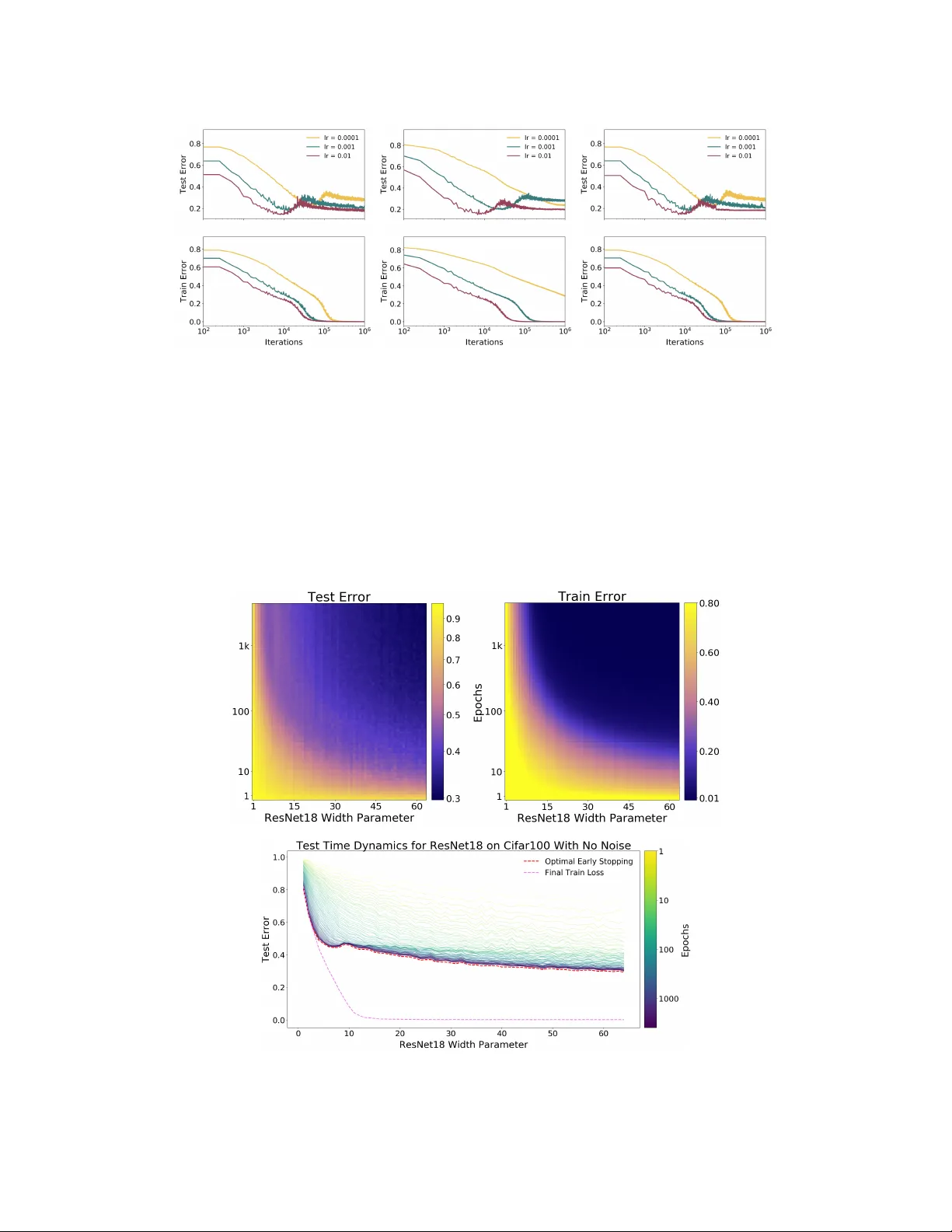
D E E P D O U B L E D E S C E N T : W H E R E B I G G E R M O D E L S A N D M O R E D A T A H U RT Preetum Nakkiran ∗ Harvard Uni versity Gal Kaplun † Harvard Uni versity Y amini Bansal † Harvard Uni versity T ristan Y ang Harvard Uni versity Boaz Barak Harvard Uni versity Ilya Sutskev er OpenAI A B S T R AC T W e show that a variety of modern deep learning tasks exhibit a “double-descent” phenomenon where, as we increase model size, performance first gets worse and then gets better . Moreov er, we show that double descent occurs not just as a function of model size, but also as a function of the number of training epochs. W e unify the above phenomena by defining a new complexity measure we call the effective model comple xity and conjecture a generalized double descent with respect to this measure. Furthermore, our notion of model complexity allo ws us to identify certain regimes where increasing (even quadrupling) the number of train samples actually hurts test performance. 1 I N T RO D U C T I O N Figure 1: Left: T rain and test error as a function of model size, for ResNet18s of varying width on CIF AR-10 with 15% label noise. Right: T est error , shown for varying train epochs. All models trained using Adam for 4K epochs. The lar gest model (width 64 ) corresponds to standard ResNet18. The bias-variance trade-of f is a fundamental concept in classical statistical learning theory (e.g., Hastie et al. (2005)). The idea is that models of higher complexity have lo wer bias but higher vari- ance. According to this theory , once model complexity passes a certain threshold, models “ov erfit” with the v ariance term dominating the test error, and hence from this point onw ard, increasing model complexity will only decrease performance (i.e., increase test error). Hence con ventional wisdom in classical statistics is that, once we pass a certain threshold, “lar ger models ar e worse. ” Howe ver , modern neural networks exhibit no such phenomenon. Such networks have millions of parameters, more than enough to fit even random labels (Zhang et al. (2016)), and yet they perform much better on many tasks than smaller models. Indeed, con ventional wisdom among practitioners is that “lar ger models are better’ ’ (Krizhe vsky et al. (2012), Huang et al. (2018), Szegedy et al. ∗ W ork performed in part while Preetum Nakkiran was interning at OpenAI, with Ilya Sutskever . W e espe- cially thank Mikhail Belkin and Christopher Olah for helpful discussions throughout this work. Correspondence Email: preetum@cs.harvard.edu † Equal contribution 1 Figure 2: Left: T est error as a function of model size and train epochs. The horizontal line corre- sponds to model-wise double descent–v arying model size while training for as long as possible. The vertical line corresponds to epoch-wise double descent, with test error undergoing double-descent as train time increases. Right T rain error of the corresponding models. All models are Resnet18s trained on CIF AR-10 with 15% label noise, data-augmentation, and Adam for up to 4K epochs. (2015), Radford et al. (2019)). The effect of training time on test performance is also up for debate. In some settings, “early stopping” improv es test performance, while in other settings training neu- ral networks to zero training error only improves performance. Finally , if there is one thing both classical statisticians and deep learning practitioners agree on is “mor e data is always better” . In this paper , we present empirical e vidence that both reconcile and challenge some of the above “con ventional wisdoms. ” W e show that many deep learning settings hav e two different regimes. In the under-par ameterized re gime, where the model complexity is small compared to the number of samples, the test error as a function of model complexity follows the U-like behavior predicted by the classical bias/variance tradeoff. Howe ver , once model complexity is sufficiently large to interpolate i.e., achieve (close to) zero training error , then increasing comple xity only decr eases test error , follo wing the modern intuition of “bigger models are better”. Similar behavior was pre viously observed in Opper (1995; 2001), Advani & Saxe (2017), Spigler et al. (2018), and Geiger et al. (2019b). This phenomenon was first postulated in generality by Belkin et al. (2018) who named it “double descent”, and demonstrated it for decision trees, random features, and 2-layer neural networks with ` 2 loss, on a variety of learning tasks including MNIST and CIF AR-10. Main contributions. W e show that double descent is a robust phenomenon that occurs in a variety of tasks, architectures, and optimization methods (see Figure 1 and Section 5; our experiments are summarized in T able A). Moreo ver , we propose a much more general notion of “double descent” that goes beyond varying the number of parameters. W e define the effective model complexity (EMC) of a training procedure as the maximum number of samples on which it can achieve close to zero training error . The EMC depends not just on the data distribution and the architecture of the classifier but also on the training procedure—and in particular increasing training time will increase the EMC. W e hypothesize that for many natural models and learning algorithms, double descent occurs as a function of the EMC. Indeed we observe “epoch-wise double descent” when we keep the model fixed and increase the training time, with performance following a classical U-like curve in the underfitting stage (when the EMC is smaller than the number of samples) and then impro ving with training time once the EMC is sufficiently lar ger than the number of samples (see Figure 2). As a corollary , early stopping only helps in the relativ ely narrow parameter re gime of critically parameterized models. Sample non-monotonicity . Finally , our results shed light on test performance as a function of the number of train samples. Since the test error peaks around the point where EMC matches the number of samples (the transition from the under- to ov er-parameterization), increasing the number of samples has the effect of shifting this peak to the right. While in most settings increasing the number of samples decreases error , this shifting effect can sometimes result in a setting where mor e data is wor se! For example, Figure 3 demonstrates cases in which increasing the number of samples by a factor of 4 . 5 results in worse test performance. 2 Figure 3: T est loss (per-token perplexity) as a function of Transformer model size (embed- ding dimension d model ) on language trans- lation (IWSL T‘14 German-to-English). The curve for 18k samples is generally lower than the one for 4k samples, but also shifted to the right, since fitting 18k samples requires a larger model. Thus, for some models, the performance for 18k samples is worse than for 4k samples. 2 O U R R E S U LT S T o state our hypothesis more precisely , we define the notion of effective model complexity . W e define a training pr ocedur e T to be any procedure that takes as input a set S = { ( x 1 , y 1 ) , . . . , ( x n , y n ) } of labeled training samples and outputs a classifier T ( S ) mapping data to labels. W e define the effective model complexity of T (w .r .t. distribution D ) to be the maximum number of samples n on which T achie ves on av erage ≈ 0 tr aining err or . Definition 1 (Effective Model Complexity) The Effecti ve Model Complexity (EMC) of a tr aining pr ocedur e T , with r espect to distribution D and par ameter > 0 , is defined as: EMC D , ( T ) := max { n | E S ∼D n [Error S ( T ( S ))] ≤ } wher e Error S ( M ) is the mean err or of model M on train samples S . Our main hypothesis can be informally stated as follo ws: Hypothesis 1 (Generalized Double Descent hypothesis, inf ormal) F or any natural data distrib u- tion D , neural-network-based training procedur e T , and small > 0 , if we consider the task of pr edicting labels based on n samples fr om D then: Under -paremeterized r egime. If EMC D , ( T ) is suf ficiently smaller than n , any perturbation of T that incr eases its effective comple xity will decrease the test err or . Over -parameterized regime. If EMC D , ( T ) is sufficiently larg er than n , any perturbation of T that incr eases its effective comple xity will decrease the test err or . Critically parameterized regime. If EMC D , ( T ) ≈ n , then a perturbation of T that incr eases its effective comple xity might decr ease or increase the test err or . Hypothesis 1 is informal in several ways. W e do not have a principled way to choose the parameter (and currently heuristically use = 0 . 1 ). W e also are yet to have a formal specification for “sufficiently smaller” and “sufficiently larger”. Our experiments suggest that there is a critical interval around the interpolation threshold when EMC D , ( T ) = n : below and above this interval increasing complexity helps performance, while within this interval it may hurt performance. The width of the critical interv al depends on both the distribution and the training procedure in w ays we do not yet completely understand. W e believ e Hypothesis 1 sheds light on the interaction between optimization algorithms, model size, and test performance and helps reconcile some of the competing intuitions about them. The main result of this paper is an experimental validation of Hypothesis 1 under a variety of settings, where we considered sev eral natural choices of datasets, architectures, and optimization algorithms, and we changed the “interpolation threshold” by v arying the number of model parameters, the length of training, the amount of label noise in the distribution, and the number of train samples. Model-wise Double Descent. In Section 5, we study the test error of models of increasing size, for a fixed large number of optimization steps. W e show that “model-wise double-descent” occurs for various modern datasets (CIF AR-10, CIF AR-100, IWSL T‘14 de-en, with varying amounts of label noise), model architectures (CNNs, ResNets, T ransformers), optimizers (SGD, Adam), number 3 of train samples, and training procedures (data-augmentation, and regularization). Moreover , the peak in test error systematically occurs at the interpolation threshold. In particular, we demonstrate realistic settings in which bigger models ar e worse . Epoch-wise Double Descent. In Section 6, we study the test error of a fixed, large architecture o ver the course of training. W e demonstrate, in similar settings as above, a corresponding peak in test performance when models are trained just long enough to reach ≈ 0 train error . The test error of a large model first decreases (at the beginning of training), then increases (around the critical regime), then decreases once more (at the end of training)—that is, training long er can correct overfitting . Sample-wise Non-monotonicity . In Section 7, we study the test error of a fix ed model and training procedure, for varying number of train samples. Consistent with our generalized double-descent hypothesis, we observe distinct test behavior in the “critical regime”, when the number of samples is near the maximum that the model can fit. This often manifests as a long plateau region, in which taking significantly more data might not help when training to completion (as is the case for CNNs on CIF AR-10). Moreov er, we show settings (Transformers on IWSL T‘14 en-de), where this manifests as a peak—and for a fixed architecture and training procedure, mor e data actually hurts. Remarks on Label Noise. W e observe all forms of double descent most strongly in settings with label noise in the train set (as is often the case when collecting train data in the real-world). How- ev er , we also sho w se veral realistic settings with a test-error peak e ven without label noise: ResNets (Figure 4a) and CNNs (Figure 20) on CIF AR-100; Transformers on IWSL T‘14 (Figure 8). More- ov er, all our e xperiments demonstrate distinctly different test behavior in the critical re gime— often manifesting as a “plateau” in the test error in the noiseless case which de velops into a peak with added label noise. See Section 8 for further discussion. 3 R E L A T E D W O R K Model-wise double descent was first proposed as a general phenomenon by Belkin et al. (2018). Similar behavior had been observed in Opper (1995; 2001), Advani & Saxe (2017), Spigler et al. (2018), and Geiger et al. (2019b). Subsequently , there has been a large body of work studying the double descent phenomenon. A growing list of papers that theoretically analyze it in the tractable setting of linear least squares regression includes Belkin et al. (2019); Hastie et al. (2019); Bartlett et al. (2019); Muthukumar et al. (2019); Bibas et al. (2019); Mitra (2019); Mei & Montanari (2019). Moreov er, Geiger et al. (2019a) provide preliminary results for model-wise double descent in con- volutional networks trained on CIF AR-10. Our work differs from the abov e papers in two crucial aspects: First, we extend the idea of double-descent beyond the number of parameters to incorpo- rate the training procedure under a unified notion of “Effecti ve Model Comple xity”, leading to no vel insights like epoch-wise double descent and sample non-monotonicity . The notion that increasing train time corresponds to increasing complexity was also presented in Nakkiran et al. (2019). Sec- ond, we provide an extensi ve and rigorous demonstration of double-descent for modern practices spanning a variety of architectures, datasets optimization procedures. An extended discussion of the related work is provided in Appendix C. 4 E X P E R I M E N TA L S E T U P W e briefly describe the experimental setup here; full details are in Appendix B 1 . W e consider three families of architectures: ResNets, standard CNNs, and T ransformers. ResNets: W e parameterize a family of ResNet18s (He et al. (2016)) by scaling the width (number of filters) of con volutional layers. Specifically , we use layer widths [ k , 2 k , 4 k, 8 k ] for varying k . The standard ResNet18 corresponds to k = 64 . Standard CNNs: W e consider a simple family of 5-layer CNNs, with 4 con volutional layers of widths [ k , 2 k , 4 k, 8 k ] for varying k , and a fully-connected layer . For context, the CNN with width k = 64 , can reach over 90% test accurac y on CIF AR-10 with data- augmentation. T ransformers: W e consider the 6 layer encoder-decoder from V aswani et al. (2017), as implemented by Ott et al. (2019). W e scale the size of the network by modifying the embedding dimension d model , and setting the width of the fully-connected layers proportionally ( d ff = 4 · d model ). 1 The raw data from our e xperiments are available at: https://gitlab.com/ harvard- machine- learning/double- descent/tree/master 4 For ResNets and CNNs, we train with cross-entropy loss, and the following optimizers: (1) Adam with learning-rate 0 . 0001 for 4K epochs; (2) SGD with learning rate ∝ 1 √ T for 500K gradient steps. W e train T ransformers for 80K gradient steps, with 10% label smoothing and no drop-out. Label Noise. In our e xperiments, label noise of probability p refers to training on a samples which hav e the correct label with probability (1 − p ) , and a uniformly random incorrect label otherwise (label noise is sampled only once and not per epoch). Figure 1 plots test error on the noisy distribu- tion, while the remaining figures plot test error with respect to the clean distribution (the two curv es are just linear rescaling of one another). 5 M O D E L - W I S E D O U B L E D E S C E N T (a) CIF AR-100. There is a peak in test error even with no label noise. (b) CIF AR-10. There is a “plateau” in test error around the interpolation point with no label noise, which dev elops into a peak for added label noise. Figure 4: Model-wise double descent f or ResNet18s. T rained on CIF AR-100 and CIF AR-10, with varying label noise. Optimized using Adam with LR 0 . 0001 for 4K epochs, and data-augmentation. In this section, we study the test error of models of increasing size, when training to completion (for a fix ed large number of optimization steps). W e demonstrate model-wise double descent across different architectures, datasets, optimizers, and training procedures. The critical region exhibits distinctly dif ferent test behavior around the interpolation point and there is often a peak in test error that becomes more prominent in settings with label noise. For the experiments in this section (Figures 4, 5, 6, 7, 8), notice that all modifications which increase the interpolation threshold (such as adding label noise, using data augmentation, and increasing the number of train samples) also correspondingly shift the peak in test error tow ards larger models. Additional plots showing the early-stopping behavior of these models, and additional experiments showing double descent in settings with no label noise (e.g. Figure 19) are in Appendix E.2. W e also observ ed model-wise double descent for adversarial training, with a prominent robust test error peak ev en in settings without label noise. See Figure 26 in Appendix E.2. Discussion. Fully understanding the mechanisms behind model-wise double descent in deep neu- ral networks remains an important open question. Howe ver , an analog of model-wise double descent occurs ev en for linear models. A recent stream of theoretical works analyzes this setting (Bartlett et al. (2019); Muthukumar et al. (2019); Belkin et al. (2019); Mei & Montanari (2019); Hastie et al. (2019)). W e believ e similar mechanisms may be at work in deep neural networks. Informally , our intuition is that for model-sizes at the interpolation threshold, there is effecti vely only one model that fits the train data and this interpolating model is very sensitiv e to noise in the 5 (a) W ithout data augmentation. (b) W ith data augmentation. Figure 5: Effect of Data A ugmentation. 5-layer CNNs on CIF AR10, with and without data- augmentation. Data-augmentation shifts the interpolation threshold to the right, shifting the test error peak accordingly . Optimized using SGD for 500K steps. See Figure 27 for larger models. Figure 6: SGD vs. Adam. 5-Layer CNNs on CIF AR-10 with no label noise, and no data augmentation. Optimized using SGD for 500K gradient steps, and Adam for 4K epochs. Figure 7: Noiseless settings. 5-layer CNNs on CIF AR-100 with no label noise; note the peak in test error . T rained with SGD and no data augmentation. See Fig- ure 20 for the early-stopping behavior of these models. train set and/or model mis-specification. That is, since the model is just barely able to fit the train data, forcing it to fit even slightly-noisy or mis-specified labels will destroy its global structure, and result in high test error . (See Figure 28 in the Appendix for an experiment demonstrating this noise sensitivity , by showing that ensembling helps significantly in the critically-parameterized regime). Howe ver for over -parameterized models, there are many interpolating models that fit the train set, and SGD is able to find one that “memorizes” (or “absorbs”) the noise while still performing well on the distribution. The above intuition is theoretically justified for linear models. In general, this situation manifests ev en without label noise for linear models (Mei & Montanari (2019)), and occurs whene ver there 6 Figure 8: T ransformers on language trans- lation tasks: Multi-head-attention encoder - decoder T ransformer model trained for 80k gradient steps with labeled smoothed cross-entropy loss on IWSL T‘14 German- to-English (160K sentences) and WMT‘14 English-to-French (subsampled to 200K sen- tences) dataset. T est loss is measured as per- token perplexity . is model mis-specification between the structure of the true distribution and the model family . W e believ e this intuition extends to deep learning as well, and it is consistent with our experiments. 6 E P O C H - W I S E D O U B L E D E S C E N T In this section, we demonstrate a novel form of double-descent with respect to training epochs, which is consistent with our unified vie w of effecti ve model comple xity (EMC) and the generalized double descent hypothesis. Increasing the train time increases the EMC—and thus a sufficiently large model transitions from under - to over -parameterized over the course of training. Figure 9: Left: Training dynamics for models in three regimes. Models are ResNet18s on CIF AR10 with 20% label noise, trained using Adam with learning rate 0 . 0001 , and data augmentation. Right: T est error over (Model size × Epochs). Three slices of this plot are shown on the left. As illustrated in Figure 9, sufficiently lar ge models can undergo a “double descent” beha vior where test error first decreases then increases near the interpolation threshold, and then decreases again. In contrast, for “medium sized” models, for which training to completion will only barely reach ≈ 0 error , the test error as a function of training time will follow a classical U-like curve where it is better to stop early . Models that are too small to reach the approximation threshold will remain in the “under parameterized” regime where increasing train time monotonically decreases test error . Our e xperiments (Figure 10) sho w that man y settings of dataset and architecture e xhibit epoch-wise double descent, in the presence of label noise. Further, this phenomenon is robust across optimizer variations and learning rate schedules (see additional experiments in Appendix E.1). As in model- wise double descent, the test error peak is accentuated with label noise. Con ventional wisdom suggests that training is split into two phases: (1) In the first phase, the net- work learns a function with a small generalization gap (2) In the second phase, the network starts to over -fit the data leading to an increase in test error . Our experiments suggest that this is not the complete picture—in some regimes, the test error decreases ag ain and may achiev e a lower v alue at the end of training as compared to the first minimum (see Fig 10 for 10% label noise). 7 (a) ResNet18 on CIF AR10. (b) ResNet18 on CIF AR100. (c) 5-layer CNN on CIF AR 10. Figure 10: Epoch-wise double descent for ResNet18 and CNN (width=128). ResNets trained using Adam with learning rate 0 . 0001 , and CNNs trained with SGD with inv erse-squareroot learning rate. 7 S A M P L E - W I S E N O N - M O N O T O N I C I T Y In this section, we in vestigate the effect of v arying the number of train samples, for a fixed model and training procedure. Previously , in model-wise and epoch-wise double descent, we explored behavior in the critical regime, where EMC D , ( T ) ≈ n , by varying the EMC. Here, we explore the critical regime by varying the number of train samples n . By increasing n , the same training procedure T can switch from being effecti vely o ver-parameterized to ef fectiv ely under-parameterized. W e show that increasing the number of samples has two dif ferent effects on the test error vs. model complexity graph. On the one hand, (as expected) increasing the number of samples shrinks the area under the curve. On the other hand, increasing the number of samples also has the effect of “shifting the curve to the right” and increasing the model comple xity at which test error peaks. (a) Model-wise double descent for 5-layer CNNs on CIF AR-10, for varying dataset sizes. T op: There is a range of model sizes (shaded green) where training on 2 × more samples does not im- prov e test error . Bottom: There is a range of model sizes (shaded red) where training on 4 × more samples does not improv e test error . (b) Sample-wise non-monotonicity . T est loss (per-w ord perplexity) as a function of number of train samples, for two transformer models trained to completion on IWSL T’14. For both model sizes, there is a regime where more samples hurt performance. Compare to Figure 3, of model-wise double-descent in the identical setting. Figure 11: Sample-wise non-monotonicity . 8 These twin ef fects are shown in Figure 11a. Note that there is a range of model sizes where the effects “cancel out”—and having 4 × more train samples does not help test performance when training to completion. Outside the critically-parameterized regime, for sufficiently under- or over - parameterized models, having more samples helps. This phenomenon is corroborated in Figure 12, which shows test error as a function of both model and sample size, in the same setting as Figure 11a. Figure 12: Left: T est Error as a function of model size and number of train samples, for 5-layer CNNs on CIF AR-10 + 20% noise. Note the ridge of high test error again lies along the interpolation threshold. Right: Three slices of the left plot, showing the effect of more data for models of different sizes. Note that, when training to completion, more data helps for small and large models, but does not help for near -critically-parameterized models (green). In some settings, these two effects combine to yield a regime of model sizes where more data actually hurts test performance as in Figure 3 (see also Figure 11b). Note that this phenomenon is not unique to DNNs: more data can hurt ev en for linear models (see Appendix D). 8 C O N C L U S I O N A N D D I S C U S S I O N W e introduce a generalized double descent hypothesis: models and training procedures exhibit atyp- ical beha vior when their Ef fective Model Complexity is comparable to the number of train samples. W e provide extensi ve evidence for our hypothesis in modern deep learning settings, and show that it is robust to choices of dataset, architecture, and training procedures. In particular , we demon- strate “model-wise double descent” for modern deep networks and characterize the regime where bigger models can perform worse. W e also demonstrate “epoch-wise double descent, ” which, to the best of our knowledge, has not been previously proposed. Finally , we show that the double descent phenomenon can lead to a regime where training on more data leads to worse test performance. Preliminary results suggest that double descent also holds as we vary the amount of regularization for a fixed model (see Figure 22). W e also believ e our characterization of the critical regime provides a useful way of thinking for practitioners—if a model and training procedure are just barely able to fit the train set, then small changes to the model or training procedure may yield unexpected behavior (e.g. making the model slightly larger or smaller , changing re gularization, etc. may hurt test performance). Early stopping. W e note that many of the phenomena that we highlight often do not occur with optimal early-stopping. Howe ver , this is consistent with our generalized double descent hypothesis: if early stopping prev ents models from reaching 0 train error then we would not expect to see double- descent, since the EMC does not reach the number of train samples. Further, we show at least one 9 setting where model-wise double descent can still occur ev en with optimal early stopping (ResNets on CIF AR-100 with no label noise, see Figure 19). W e hav e not observed settings where more data hurts when optimal early-stopping is used. Howe ver , we are not aware of reasons which preclude this from occurring. W e leav e fully understanding the optimal early stopping behavior of double descent as an important open question for future work. Label Noise. In our experiments, we observe double descent most strongly in settings with label noise. Howe ver , we believe this effect is not fundamentally about label noise, but rather about model mis-specification . For example, consider a setting where the label noise is not truly random, but rather pseudorandom (with respect to the family of classifiers being trained). In this setting, the performance of the Bayes optimal classifier would not change (since the pseudorandom noise is deterministic, and inv ertible), but we would observe an identical double descent as with truly random label noise. Thus, we view adding label noise as merely a proxy for making distributions “harder”— i.e. increasing the amount of model mis-specification. Other Notions of Model Complexity . Our notion of Effective Model Complexity is related to classical complexity notions such as Rademacher complexity , but differs in sev eral crucial ways: (1) EMC depends on the true labels of the data distribution, and (2) EMC depends on the training procedure, not just the model architecture. Other notions of model complexity which do not incorporate features (1) and (2) would not suffice to characterize the location of the double-descent peak. Rademacher complexity , for example, is determined by the ability of a model architecture to fit a randomly-labeled train set. But Rademacher complexity and VC dimension are both insufficient to determine the model-wise double descent peak location, since they do not depend on the distribution of labels— and our experiments show that adding label noise shifts the location of the peak. Moreov er, both Rademacher complexity and VC dimension depend only on the model family and data distribution, and not on the training procedure used to find models. Thus, they are not capable of capturing train-time double-descent effects, such as “epoch-wise” double descent, and the effect of data-augmentation on the peak location. A C K N O W L E D G M E N T S W e thank Mikhail Belkin for extremely useful discussions in the early stages of this work. W e thank Christopher Olah for suggesting the Model Size × Epoch visualization, which led to the in vestigation of epoch-wise double descent, as well as for useful discussion and feedback. W e also thank Alec Radford, Jacob Steinhardt, and V aishaal Shankar for helpful discussion and suggestions. P .N. thanks OpenAI, the Simons Institute, and the Harv ard Theory Group for a research environment that enabled this kind of work. W e thank Dimitris Kalimeris, Benjamin L. Edelman, and Sharon Qian, and Aditya Ramesh for comments on an early draft of this work. This work supported in part by NSF grant CAREER CCF 1452961, BSF grant 2014389, NSF US- ICCS proposal 1540428, a Google Research aw ard, a Facebook research award, a Simons In vestiga- tor A ward, a Simons In vestigator Fellowship, and NSF A wards CCF 1715187, CCF 1565264, CCF 1301976, IIS 1409097, and CNS 1618026. Y .B. would like to thank the MIT -IBM W atson AI Lab for contributing computational resources for e xperiments. R E F E R E N C E S Madhu S Adv ani and Andrew M Sax e. High-dimensional dynamics of generalization error in neural networks. arXiv pr eprint arXiv:1710.03667 , 2017. Peter L Bartlett, Philip M Long, G ´ abor Lugosi, and Alexander Tsigler . Benign overfitting in linear regression. arXiv pr eprint arXiv:1906.11300 , 2019. Mikhail Belkin, Daniel Hsu, Siyuan Ma, and Soumik Mandal. Reconciling modern machine learning and the bias-variance trade-of f. arXiv preprint , 2018. 10 Mikhail Belkin, Daniel Hsu, and Ji Xu. T wo models of double descent for weak features. arXiv pr eprint arXiv:1903.07571 , 2019. K oby Bibas, Y ani v Fogel, and Meir Feder . A new look at an old problem: A univ ersal learning approach to linear regression. arXiv pr eprint arXiv:1905.04708 , 2019. Mauro Cettolo, Christian Girardi, and Marcello Federico. W it 3 : W eb in ventory of transcribed and translated talks. In Pr oceedings of the 16 th Confer ence of the Eur opean Association for Machine T ranslation (EAMT) , pp. 261–268, T rento, Italy , May 2012. Mario Geiger, Arthur Jacot, Stefano Spigler , Franck Gabriel, Levent Sagun, St ´ ephane d’Ascoli, Giulio Biroli, Cl ´ ement Hongler , and Matthieu W yart. Scaling description of generalization with number of parameters in deep learning. arXiv preprint , 2019a. Mario Geiger , Stefano Spigler , St ´ ephane d’Ascoli, Lev ent Sagun, Marco Baity-Jesi, Giulio Biroli, and Matthieu W yart. Jamming transition as a paradigm to understand the loss landscape of deep neural networks. Physical Review E , 100(1):012115, 2019b. Ian J Goodfellow , Jonathon Shlens, and Christian Szegedy . Explaining and harnessing adversarial examples. arXiv pr eprint arXiv:1412.6572 , 2014. T rev or Hastie, Robert T ibshirani, Jerome Friedman, and James Franklin. The elements of statistical learning: data mining, inference and prediction. The Mathematical Intelligencer , 27(2):83–85, 2005. T rev or Hastie, Andrea Montanari, Saharon Rosset, and Ryan J Tibshirani. Surprises in high- dimensional ridgeless least squares interpolation. arXiv preprint , 2019. Kaiming He, Xiangyu Zhang, Shaoqing Ren, and Jian Sun. Identity mappings in deep residual networks. In Eur opean confer ence on computer vision , pp. 630–645. Springer, 2016. Y anping Huang, Y onglong Cheng, Dehao Chen, HyoukJoong Lee, Jiquan Ngiam, Quoc V . Le, and Zhifeng Chen. Gpipe: Efficient training of giant neural networks using pipeline parallelism. CoRR , abs/1811.06965, 2018. URL . Alex Krizhe vsky . Learning multiple layers of features from tiny images. T echnical report, 2009. Alex Krizhevsk y , Ilya Sutskev er, and Geof frey E Hinton. Imagenet classification with deep conv o- lutional neural networks. In Advances in neural information pr ocessing systems , pp. 1097–1105, 2012. Aleksander Madry , Aleksandar Makelov , Ludwig Schmidt, Dimitris Tsipras, and Adrian Vladu. T ow ards deep learning models resistant to adversarial attacks. arXiv preprint , 2017. Song Mei and Andrea Montanari. The generalization error of random features regression: Precise asymptotics and double descent curve. arXiv pr eprint arXiv:1908.05355 , 2019. Partha P . Mitra. Understanding overfitting peaks in generalization error: Analytical risk curves for l2 and l1 penalized interpolation. ArXiv , abs/1906.03667, 2019. V idya Muthukumar , Kailas V odrahalli, and Anant Sahai. Harmless interpolation of noisy data in regression. arXiv pr eprint arXiv:1903.09139 , 2019. Preetum Nakkiran, Gal Kaplun, Dimitris Kalimeris, Tristan Y ang, Benjamin L Edelman, Fred Zhang, and Boaz Barak. Sgd on neural netw orks learns functions of increasing complexity . arXiv pr eprint arXiv:1905.11604 , 2019. Manfred Opper . Statistical mechanics of learning: Generalization. The Handbook of Brain Theory and Neural Networks, 922-925. , 1995. Manfred Opper . Learning to generalize. F r ontiers of Life, 3(part 2), pp.763-775. , 2001. 11 Myle Ott, Serge y Edunov , Alexei Baevski, Angela Fan, Sam Gross, Nathan Ng, David Grangier , and Michael Auli. fairseq: A fast, extensible toolkit for sequence modeling. In Pr oceedings of N AACL-HL T 2019: Demonstr ations , 2019. David Page. How to train your resnet. https://myrtle.ai/ how- to- train- your- resnet- 4- architecture/ , 2018. Adam Paszke, Sam Gross, Soumith Chintala, Gregory Chanan, Edward Y ang, Zachary DeV ito, Zeming Lin, Alban Desmaison, Luca Antiga, and Adam Lerer . Automatic differentiation in PyT orch. In NeurIPS Autodiff W orkshop , 2017. Alec Radford, Jeff W u, Rew on Child, David Luan, Dario Amodei, and Ilya Sutske ver . Language models are unsupervised multitask learners. 2019. Ali Rahimi and Benjamin Recht. Random features for large-scale kernel machines. In Advances in neural information pr ocessing systems , pp. 1177–1184, 2008. Rico Sennrich, Barry Haddow , and Ale xandra Birch. Neural machine translation of rare words with subword units. ArXiv , abs/1508.07909, 2015. Stefano Spigler , Mario Geiger , St ´ ephane d’Ascoli, Le vent Sagun, Giulio Biroli, and Matthieu W yart. A jamming transition from under-to over -parametrization affects loss landscape and generaliza- tion. arXiv preprint , 2018. Christian Szegedy , W ei Liu, Y angqing Jia, Pierre Sermanet, Scott Reed, Dragomir Anguelov , Du- mitru Erhan, V incent V anhoucke, and Andrew Rabinovich. Going deeper with conv olutions. In Computer V ision and P attern Recognition (CVPR) , 2015. URL 1409.4842 . Ashish V aswani, Noam Shazeer, Niki Parmar , Jakob Uszkoreit, Llion Jones, Aidan N. Gomez, Lukasz Kaiser , and Illia Polosukhin. Attention is all you need. CoRR , abs/1706.03762, 2017. Chiyuan Zhang, Samy Bengio, Moritz Hardt, Benjamin Recht, and Oriol V inyals. Understanding deep learning requires rethinking generalization. ICLR , abs/1611.03530, 2016. 12 A S U M M A RY TA B L E O F E X P E R I M E N TA L R E S U LT S Double-Descent Dataset Architecture Opt. Aug. % Noise Model Epoch Figure(s) CIF AR 10 CNN SGD X 0 7 7 5, 27 X 10 X X 5, 27, 6 X 20 X X 5, 27 0 7 7 5, 25 10 X X 5 20 X X 5 SGD + w .d. X 20 X X 21 Adam 0 X – 25 ResNet Adam X 0 7 7 4, 10 X 5 X – 4 X 10 X X 4, 10 X 15 X X 4, 2 X 20 X X 4, 9, 10 V arious X 20 – X 16, 17, 18 (subsampled) CNN SGD X 10 X – 11a SGD X 20 X – 11a, 12 (adversarial) ResNet SGD 0 Robust err . – 26 CIF AR 100 ResNet Adam X 0 X 7 4, 19, 10 X 10 X X 4, 10 X 20 X X 4, 10 CNN SGD 0 X 7 20 IWSL T ’14 de-en T ransformer Adam 0 X 7 8, 24 (subsampled) T ransformer Adam 0 X 7 11b, 23 WMT ’14 en-fr T ransformer Adam 0 X 7 8, 24 B A P P E N D I X : E X P E R I M E N TA L D E T A I L S B . 1 M O D E L S W e use the follo wing families of architectures. The PyT orch Paszke et al. (2017) specification of our ResNets and CNNs are a vailable at https://gitlab.com/ harvard- machine- learning/double- descent/tree/master . ResNets. W e define a family of ResNet18s of increasing size as follo ws. W e follo w the Preac- tiv ation ResNet18 architecture of He et al. (2016), using 4 ResNet blocks, each consisting of two BatchNorm-ReLU-Con volution layers. The layer widths for the 4 blocks are [ k , 2 k , 4 k, 8 k ] for varying k ∈ N and the strides are [1, 2, 2, 2]. The standard ResNet18 corresponds to k = 64 con- volutional channels in the first layer . The scaling of model size with k is shown in Figure 13b. Our implementation is adapted from https://github.com/kuangliu/pytorch- cifar . Standard CNNs. W e consider a simple family of 5-layer CNNs, with four Con v-BatchNorm- ReLU-MaxPool layers and a fully-connected output layer . W e scale the four con volutional layer widths as [ k , 2 k, 4 k , 8 k ] . The MaxPool is [1, 2, 2, 8]. For all the con volution layers, the kernel size = 3, stride = 1 and padding=1. This architecture is based on the “backbone” architecture from Page (2018). For k = 64 , this CNN has 1558026 parameters and can reach > 90% test accuracy on CIF AR-10 (Krizhevsk y (2009)) with data-augmentation. The scaling of model size with k is sho wn in Figure 13a. T ransformers. W e consider the encoder-decoder Transformer model from V aswani et al. (2017) with 6 layers and 8 attention heads per layer , as implemented by fairseq Ott et al. (2019). W e scale the size of the network by modifying the embedding dimension ( d model ), and scale the width of the fully-connected layers proportionally ( d ff = 4 d model ). W e train with 10% label smoothing and no drop-out, for 80 gradient steps. 13 (a) 5-layer CNNs (b) ResNet18s (c) T ransformers Figure 13: Scaling of model size with our parameterization of width & embedding dimension. B . 2 I M A G E C L A S S I FI C A T I O N : E X P E R I M E N TA L S E T U P W e describe the details of training for CNNs and ResNets below . Loss function: Unless stated otherwise, we use the cross-entropy loss for all the experiments. Data-augmentation: In experiments where data-augmentation was used, we apply RandomCrop(32, padding=4) and RandomHorizontalFlip . In experiments with added label noise, the label for all augmentations of a giv en training sample are given the same label. Regularization: No explicit regularization like weight decay or dropout was applied unless explic- itly stated. Initialization: W e use the default initialization provided by PyT orch for all the layers. Optimization: • Adam: Unless specified otherwise, learning rate was set at constant to 1e − 4 and all other parameters were set to their default PyT orch values. • SGD: Unless specified otherwise, learning rate schedule in verse-square root (defined be- low) was used with initial learning rate γ 0 = 0 . 1 and updates ev ery L = 512 gradient s teps. No momentum was used. W e found our results are robust to various other natural choices of optimizers and learning rate schedule. W e used the above settings because (1) the y optimize well, and (2) they do not require experiment-specific hyperparameter tuning, and allow us to use the same optimization across many experiments. Batch size : All experiments use a batchsize of 128. Learning rate schedule descriptions: • In verse-squar e root ( γ 0 , L ) : At gradient step t , the learning rate is set to γ ( t ) := γ 0 √ 1+ b t/ 512 c . W e set learning-rate with respect to number of gradient steps, and not epochs, in order to allow comparison between e xperiments with varying train-set sizes. • Dynamic dr op ( γ 0 , drop, patience) : Starts with an initial learning rate of γ 0 and drops by a factor of ’ drop’ if the training loss has remained constant or become worse for ’patience’ number of gradient steps. B . 3 N E U R A L M A C H I N E T R A N S L A T I O N : E X P E R I M E N TA L S E T U P Here we describe the experimental setup for the neural machine translation e xperiments. T raining procedure. 14 In this setting, the distribution D consists of triples ( x, y , i ) : x ∈ V ∗ src , y ∈ V ∗ tg t , i ∈ { 0 , . . . , | y |} where V src and V tg t are the source and target vocabularies, the string x is a sentence in the source language, y is its translation in the tar get language, and i is the inde x of the token to be predicted by the model. W e assume that i | x, y is distributed uniformly on { 0 , . . . , | y |} . A standard probabilistic model defines an autoregressi ve factorization of the lik elihood: p M ( y | x ) = | y | Y i =1 p M ( y i | y
Original Paper
Loading high-quality paper...
Comments & Academic Discussion
Loading comments...
Leave a Comment