Long Distance Relationships without Time Travel: Boosting the Performance of a Sparse Predictive Autoencoder in Sequence Modeling
In sequence learning tasks such as language modelling, Recurrent Neural Networks must learn relationships between input features separated by time. State of the art models such as LSTM and Transformer are trained by backpropagation of losses into pri…
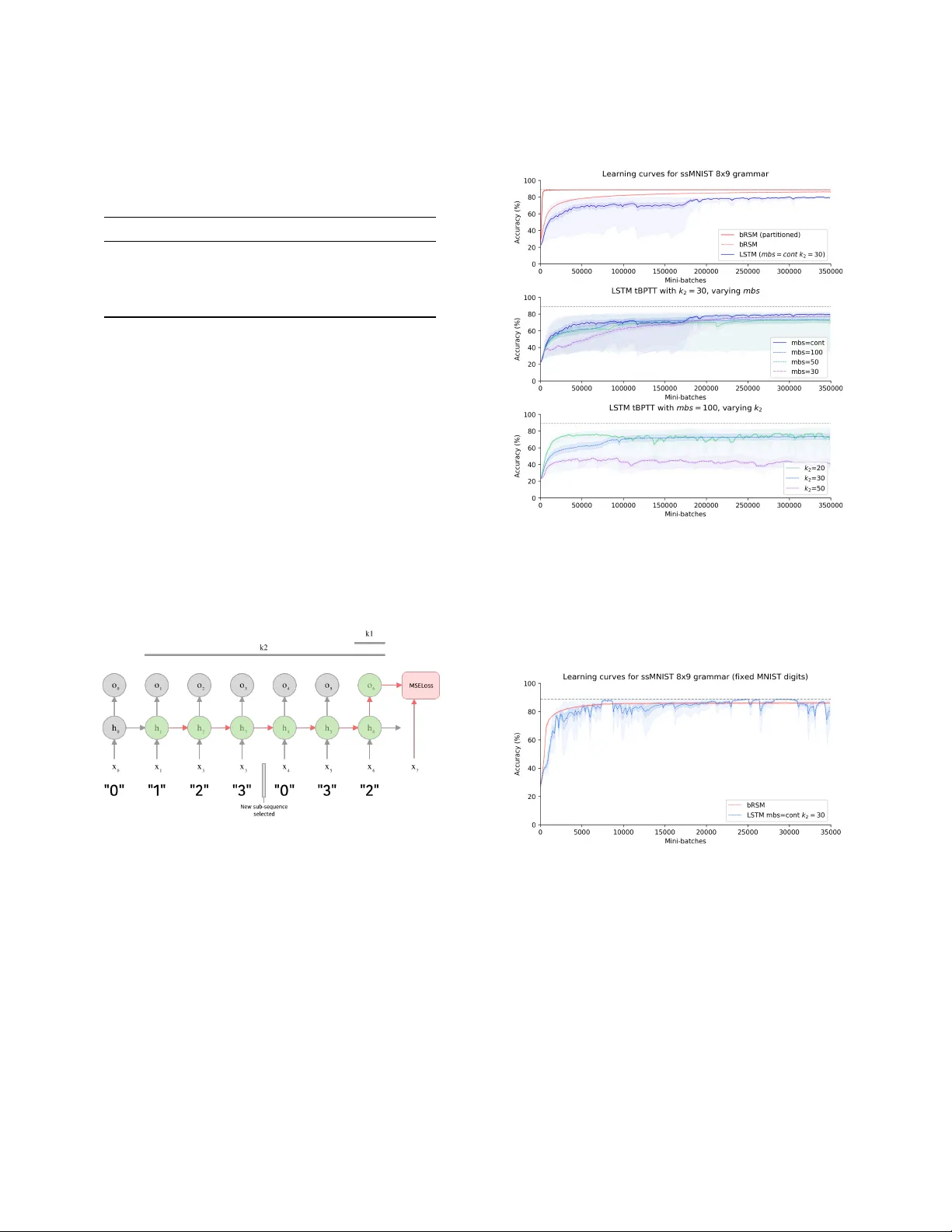
Authors: Jeremy Gordon, David Rawlinson, Subutai Ahmad
Long Distance Relationships without Time T ravel: Boosting the Performance of a Sparse Predictive A utoencoder in Se quence Modeling Jeremy Gordon UC Berkeley & Numenta jrgordon@berkeley .edu David Rawlinson Incubator 491 dave@agi.io Subutai Ahmad Numenta sahmad@numenta.com ABSTRA CT In sequence learning tasks such as language modelling, Recurrent Neural Networks must learn relationships between input features separated by time. State of the art models such as LSTM and Trans- former are trained by backpropagation of losses into prior hidden states and inputs held in memory . This allows gradients to ow from present to past and eectively learn with perfect hindsight, but at a signicant memory cost. In this paper we show that it is possible to train high performance recurrent networks using in- formation that is local in time, and thereby achieve a signicantly reduced memory footprint. W e describe a predictive autoencoder called bRSM featuring recurrent connections, sparse activations, and a boosting rule for improved cell utilization. The architecture demonstrates near optimal performance on a non-deterministic (stochastic) partially-observable sequence learning task consisting of high-Markov-order sequences of MNIST digits. W e nd that this model learns these se quences faster and more completely than an LSTM, and oer several possible explanations why the LSTM architecture might struggle with the partially observable se quence structure in this task. W e also apply our model to a next word prediction task on the Penn Treebank (PTB) dataset. W e show that a ‘attened’ RSM network, when pair ed with a modern semantic word embedding and the addition of boosting, achieves 103.5 PPL (a 20-point improvement over the best N-gram models), beating ordi- nary RNNs traine d with BPT T and approaching the scores of early LSTM implementations. This work provides encouraging evidence that str ong r esults on challenging tasks such as language modelling may be possible using less memor y intensive, biologically-plausible training regimes. 1 IN TRODUCTION In the sequence learning domain, the challenge of modeling r ela- tionships b etween related elements separate d by long temporal distances is well known. Language modeling, the task of next char- acter or next wor d prediction, is an extensively studied paradigm that exhibits the need to capture such long-distance relationships that are inherent to natural language. Historically , a variety of archi- tectures have achieved excellent language modelling performance. Although larger datasets and increased memor y capacity have also improved results, architectural changes have been associated with more signicant improv ements on older benchmarks. N-gram models are an intuitive baseline model and were dev el- oped early in this history . N-gram models learn a distribution over W ork completed while the rst author was completing a summer placement with Numenta. the corpus vocabular y conditioned on the n prior tokens, e.g. a tri-gram ( n = 3 ) model makes predictions based on the distribution: P ( x i | x t − 3 , x t − 2 , x t − 1 ) = f ( x t − 3 , x t − 2 , x t − 1 ) Among N-gram models, smo othed 5-gram models achieve mini- mum perplexity on the Penn Tr eebank dataset [ 11 ], a result that illustrates constraints on the value of incr easingly long temporal context. More recent approaches have demonstrated the success of neural models such as Recurrent Neural Networks applie d to language modeling. In 2011, Mikolov et al. presented a review of language models on the Penn T ree-bank (PTB) corpus showing that recurrent neural models at that time outp erformed all other architectures [15]. Ordinary RNNs are known to suer from the vanishing gradi- ent problem in which partial derivatives used to backpropagate error signals across many layers approach zero. Hochreiter et al introduced a novel multi-gate architecture called Long Short-T erm Memory (LSTM) as a potential solution [ 9 ]. Mo dels featuring LSTM have demonstrated state of the art results in language modeling, demonstrating their ability to robustly learn long-range causal structure in sequential input. Though RNNs appear to be a natural t for language modeling due to the inherently sequential nature of the task, feed-forward networks utilizing novel convolutional strategies have also be en competitive in recent years. W aveNet is a deep autoregressive model using dilated causal convolutions in order to achieve long temporal range receptive elds [ 17 ]. A recent review compared the wider fam- ily of temporal convolutional networks (TCN)—of which W aveNet is a member—with recurrent architectures such as LSTM and GRU, nding that TCNs surpassed traditional recurrent models on a wide range of sequence learning tasks [2]. Extending the concept of replacing recurrence with autoregres- sive convolution, V aswani et al. added attentional ltering to their Transformer netw ork [ 18 ]. The Transformer uses a deep enco der and de coder each composed of multi-headed attention and feed- forward layers. While the dilated conv olutions of W aveNet allow it to learn relationships across longer temporal windows, attention allows the network to learn which parts of the input, as well as intermediate hidden states, are most useful for the present output. Current state-of-the-art results are achieved by GPT -2, a 1.5 billion parameter Transformer [ 5 ], which obtains 35.7 PPL on the PTB task (see T able 2). The previous state of the art was an LSTM with the addition of mutual gating of the current input and the previous output reporting 44.8 PPL [12]. Jeremy Gordon, David Rawlinson, and Subutai Ahmad Common to all the neural approaches r eviewed here is the use of some form of deep-backpropagation, either by unrolling through time (see section 3.1.2 for mor e detail) or through a nite window of recent inputs (W aveNet, Transformer). Since most of these models also benet from deep multilayer architectures, backpr opagation must ow across layers, and over time steps or input positions, resulting in very large computational graphs across which gradients much ow . By contrast, all other metho ds in the literature (such as traditional feed-forward ANNs and N-gram models) are not known to produce such good performance (i.e. none have surpassed 100 PPL on PTB). 1.1 Motivation Despite the impressive successes of the recurrent, autoregressive , and attention-based approaches re viewed above, the question re- mains whether similar performance can be achieved by models that do not dep end on deep backpropagation. Models that avoid backpropagation across many lay ers or time steps are interesting for two reasons. First, computational eciency is b ecoming an increasingly important consideration in deep learning, both due to the pragmatics of designing algorithms that must be trained in resource constrained environments such as edge computing, and as researchers begin to acknowledge the signicant environmental footprint of the hardware that drives machine learning at scale [ 6 ]. Second, to the extent that computational models may help us bet- ter understand the dynamics and perhaps me chanisms underlying our own cognitive abilities, architectures constrained by similar principles as those that govern the brain may oer more credible insights. Specically , we are interested in models that lie within the biologically plausible criteria outlined by Rawlinson et al.: 1) lo cal and imme diate credit assignment, 2) no synaptic memor y , and 3) no time-traveling synapses [ 16 ]. Our goal, then, is to explor e and push the performance bounds of sequence learning models leveraging dynamics consistent with these bio-plausibility constraints. 2 METHOD 2.1 Original RSM Mo del W e began with the Recurrent Sparse Memory (RSM) architecture proposed by Rawlinson et al. [ 16 ]. RSM is a predictive recurrent autoencoder that receives sequential inputs (e.g. images or word tokens), and is trained to generate a prediction of the next item in the sequence (see schematic in Figure 1). Like Hierarchical T emporal Memory [ 7 ], the RSM memory is organized into m groups ( or mini- columns), each composed of n cells. Cells within each group share a single set of weights from feed for ward input, such that the feed- forward contribution z A is an m -dimensional vector computed as: z A = w A x A ( t ) Each cell receives dense recurrent connections from all cells at the previous time step, and the r ecurrent contribution z B is an m × n matrix computed as: z B = w B x B ( t ) σ i j is an m × n matrix holding the weighted sum combining feed-for ward and recurrent input to each cell j in group i , and is given by: σ i j = z A i + z B i j A top- k sparsity is used as per Makzhani and Frey [ 10 ]. RSM implements this sparsity by computing tw o sparse binary masks, M π and M λ , which indicate the most active cell (one per group), and most active group ( k per layer), respectively . An inhibition trace was used in the original model to encourage ecient resource utilization during the sparsening step, but is replaced with boosting in this work (see section 3.2.4 for discussion). The nal output is calculated by applying a t anh nonlinearity to the sparsened activity: y i j = tanh ( σ i j · M λ i · M π i j ) A memory trace ψ ( t ) is maintained with an exponential decay parameterized by ϵ , such that ψ ( t ) = max ( ψ ( t − 1 ) · ϵ , y ) . From ψ , the recurrent input at the next time step is calculated by normalizing with constant α , chosen such that the activity in x B sums to 1: x B ( t + 1 ) = α · ψ ( t ) Like other predictive autoencoders, RSM is trained to generate the next input ˆ x A by “decoding” from the max of each group’s sparse activity: y λ i = max ( y i 1 , . . . , y i n ) The prediction is then computed as ˆ x A ( t ) = w D y λ , where w D is a weight matrix with dimension equal to the transpose of w A . Finally , to read out labels or word distributions from the network, RSM uses a simple classier netw ork composed of a 2-layer fully connected ANN using leaky ReLU nonlinearities. The classier network is traine d concurrently but independently to the RSM network (not sharing gradients), and takes the RSM’s hidden state as input. 2.2 Boosted RSM (bRSM) W e developed a variant of RSM that (among other architectural changes) replaces cell-inhibition with a cell activity ‘b oosting’ scheme. For brevity , we refer to the modied algorithm as bRSM. In an attempt to encourage better generalization, we explored a number of adjustments to the original model described in section 2.1. Additional mo del details and hyper-parameter settings for reported experiments are included in Appendix B, and the full code for all experiments is publicly accessible 1 . W e nd that bRSM signicantly improv es performance on the language modeling task. W e review each of our adjustments in the section below . 2.2.1 Flaened network. A fundamental dynamic of H TM-like ar- chitectures is that each mini-column learns some spatial structure in the input, and each cell within a mini-column learns a transi- tion from a prior repr esentation [ 8 ]. A potential limitation of this architecture is that, while representations of the input via feed for- ward connections benet from spatial semantics (similar represen- tations for similar inputs), the pr edictive representations developed through recurrent connections lack this property: similar sequence items in dierent sequential contexts are highly orthogonal [16]. 1 The full code for the bRSM model and all experiments is available at https://github. com/numenta/nupic.research/tree/master/projects/rsm Long Distance Relationships without Time Travel: Boosting the Performance of a Sparse Predictive Autoencoder in Sequence Modeling Figure 1: Schematic of original RSM architecture, shown pro- cessing inputs from the stochastic se quential MNIST task (see section 3.1.1). Note that, as per original pap er , the RSM network is trained only on the MSE loss, and is not aected by gradients backpropagated from the classier network. T o illustrate a potential ineciency of this orthogonality , con- sider a network trained on sequences where some set of similar inputs A = { A 1 , A 2 , A 3 } predict both B and C at the next time step, prompting cells in the repr esentations of both B and C to activate when exposed to inputs in A . These cells may contain nearly iden- tical weights linked to a sparse representation generalizing across patterns in A . Such a redundancy might be avoided if some sub- set of cells having learned the transition from A could be shared by both B and C . This line of reasoning motivated experiments in which each group was set to have only one cell, thus removing shared feed-for ward w eights from the model, and enabling decod- ing from the full hidden state rather than a group-max bottleneck. The exibility of allowing predictive cells to participate in multiple input representations may explain the improved p erformance of this attened architecture in the language modeling task, though we susp ect the grouped model may be benecial on tasks with higher-order compositionality in space or time. 2.2.2 Boosting. Sparse networks may learn locally optimal cong- urations in which only a small fraction of a lay er’s representational capacity is used. When this o ccurs, many units r emain idle resulting in inecient resource usage and limited performance. The original RSM model employs an inhibition strategy whereby a separate exponentially decaying trace is used to discourage recently active cells from re-activating. An alternative strategy kno wn as boosting has been proposed to achieve the same goal but exhibits dierent properties from inhibition. W e used a boosted k- Winners algorithm suggested by Cui et al. [ 1 ]. This algorithm tracks the duty cycle of each cell d i , which captures the probability of recent activation ( sparsened via top- k masking): d i ( t ) = ( 1 − α ) · d i ( t − 1 ) + α [ i ∈ t opI ndi c es ] A per-cell boost term b i is then computed based on this duty cycle, incr easing the probability of less recently active cells from ring, and inhibiting those more recently active: b i ( t ) = e β ( ˆ a − d i ( t )) where ˆ a is the expected layer sparseness dened as the number of winners divided by the layer size, k m n , and β is the boost strength hyper-parameter which can be optionally congured to remain xed or decay during training (see Appendix B). The p er-cell weighted sum σ i j is then redened as: σ i j = ( z A i + z B i j ) · b i 2.2.3 Semantic embedding. Rawlinson et al. tested RSM with a syn- thetic binar y word embedding (see Appendix C.1) with no semantic properties in order to isolate the performance of the architecture from that of the emb edding. Since RSM was not spe cically de- signed to learn high quality language embe ddings, we chose to use a modern embedding leveraging sub-word semantics. W e pre- trained a 100-dimensional FastT ext [ 4 ] embedding on the training corpus, and use d this as input for all experiments (see App endix C.2 for generation details). 2.2.4 T rainable decay . In language modeling, some tokens may provide useful conte xt to word prediction many tokens in the fu- ture (e .g. rare words unique to a particular topic), while others may be necessar y for next word prediction (e .g. tokens composing multi-word proper nouns or phrases, or common words indicating syntactic structure). In the original RSM model, the rate of decay of the recurrent input is parameterize d by a single scalar value ϵ , which is multiplied into the prior memor y state on each time step. While each cell participates in multiple input representations, it may b e possible to improve generalization performance by learning a unique exponential decay scalar for each cell in the memor y . W e implemented trainable de cay as a single tensor ∆ of dimension m ∗ n (equivalent to just m in the attened architecture), which we pass through a Sigmoid b efore applying to the memor y in the de cay step: ψ ( t + 1 ) = ψ ( t ) · σ ( ∆ ) W e found that applying a ceiling close to 1 to the σ ( ∆ ) term helped to avoid volatility likely caused by the memor y state retain- ing too much history . The benet of moving to a trainable decay parameter r equires a nominal increase in parameters, and provides a consistent but small improvement ( ~5 PPL on next word prediction). 2.2.5 Functional Partitioning. W e found one nal addition to be signicantly benecial on the stochastic se quential MNIST task (detailed in section 3.1.1). In this version of the mo del, the bRSM memory is partitioned into either two or three blocks: one taking Jeremy Gordon, David Rawlinson, and Subutai Ahmad feed-for ward input only , one taking recurrent input only , and one integrating b oth input sources via addition. This third section is equivalent to the full memory in the original RSM model. T o ensure utilization across all partitions while keeping target sparsity consis- tent, we applied the top-k nonlinearity to each partition separately , with partition winners k p proportional to partition cell count m p : k p = k m p m The motivation behind functional partitioning was an extension of the logic behind the use of a attene d memor y . T o the extent that it is useful for some cells to represent transitions from prior input, and others to represent current input, we wondered if an architecture in which these functional roles are enforced would improve performance. The partitioned model whose ssMNIST results appear in Figure 4 uses a memory with cells allocated as follows: 7% feed-for ward, 85% recurrent, and 8% integrate d. The resultant model contains fewer parameters since a portion of cells are connected only to the input, which has lower dimensionality than the full memory . This partitioning method did not improve generalization on the language modeling task hence these results are not reported. 3 EXPERIMEN TS 3.1 T asks & Datasets W e selected tasks anticipated to be dicult for RNNs and RSM in particular , to enable empirical characterization of its limitations. W e tested bRSM on two tasks: a non-deterministic version of the original partially-observable MNIST sequence task [ 16 ], as well as next word prediction ( language modeling) on the Penn T reebank dataset. 3.1.1 Stochastic Sequential MNIST ( ssMNIST). RSM was initially tested on a partially obser vable sequence learning task in which the network is exposed to higher-order sequences of randomly chosen MNIST images drawn according to a predetermined list of labels e.g. “0123 0123 0321” . It is then possible that algorithms could learn to ignore the images and simply keep count to make accurate predictions. A potential expansion to this task, then, is to require memorization of repeatable sub-sequences (e.g. the 12 digit example above) presented in a random order . This requires repeatable sub- sequences to b e learned, while also learning to ignor e sub-sequence order that has no predictive value. The image-observations and transitions are then both partially non-deterministic, and the images must be considered for optimal accuracy . These randomly ordered sub-sequences can b e described by a grammar . The grammar generating process is congur ed to specify m sub-sequences of length n digits each. Details of the grammar generated are described in Appendix A. Using a single xed grammar we can construct an observation generating process that randomly cho oses between sub-sequences, but then follows each sub-sequence deterministically , as follows: (1) Select one sub-sequence from the m specied uniformly at random (2) Select the rst digit label in the sub-sequence (3) Select a random MNIST digit according to the selecte d label (4) Move through the sub-sequence, drawing random MNIST digits for each label, until the end is reached (5) Go to 1 W e generated a test grammar comp osed of 8 sub-sequences of 9 MNIST digits each (dimension specied to minimize confusion, see sample sequence and predicted outputs in Figure 2). This specic “8x9” grammar for which we report results, along with a calcula- tion for the theoretical limit on prediction accuracy , is included in Appendix A. Figure 2: High-order , partially observable stochastic se- quence learning predictions. Rows alternate b etween actual 9-digit samples from the grammar , and bRSM predictions. Sequences “6-4-1-3-9" and “3-4-1-3-1" (with common sub- sequence “4-1-3" outlined) are predicted correctly . T o ensure that solving the task would require the successful learning of higher order sequences, we conrme d that prediction of at least some of the transitions in the resultant grammar required knowledge of the sequence item two or more steps prior . Unlike many RNN tasks, there is no ag or sp ecial token to indicate sub-sequence boundaries or task reset. Without any priors for the length or existence of sub-sequences, the ssMNIST task is challenging even for humans. 3.1.2 Baseline: tBPT T traine d LSTM. W e chose to use an LSTM as a ‘baseline’ algorithm to represent the de ep-backpropagation approach and compare to bRSM. Modern recurrent neural netw orks such as LSTMs are trained using backpropagation through time (BPT T), which conceptually unrolls the network’s computational graph across multiple time steps resulting in a standard multi-layer feed-for ward network, and then backpropagating the loss from one or more output layers (or heads) towar ds the shallower layers representing earlier timesteps. The LSTM was trained with Adam using a learning rate of 2 × 10 − 5 . W e set the hidden size of the LSTM layer to produce networks roughly consistent with the parameter count of bRSM. Results reported below are for an LSTM with 450 hidden units (2.57M parameters). W e implemented a training r egime consistent with Williams and Peng’s improved truncated-BPT T algorithm [ 19 ] which is parame- terized by two integers determining the ow of gradients through past states of the network. In t BP T T ( k 1 , k 2 ) , k 1 species the interval at which to inject error from the last k 1 outputs, while k 2 species the length of the history through which gradients should propa- gate. W e set k 1 = 1 to match the online “one digit, one prediction” Long Distance Relationships without Time Travel: Boosting the Performance of a Sparse Predictive Autoencoder in Sequence Modeling T able 1: ssMNIST results on 8x9 grammar . A ccuracy is re- ported as mean ± one standard deviation, and max over 5 runs to account for obser ved inter-run variance. Theoretical ceiling on accuracy for this grammar is 88.8%. Model Params Mean Acc Max Acc LSTM (cont) 2.6M 80.0% ± 9.1 81.4% LSTM (mbs=100) 2.6M 73.4% ± 18.2 82.7% bRSM 2.5M 86.4% ± 0.3 86.8% bRSM (partitioned) 1.8M 88.8% ± 0.1 88.9% dynamic of the ssMNIST task. After disappointing initial results with large k 2 values, we experimented with a range of values to empirically optimize LSTM performance (see schematic in Figure 3). T o conrm correctness of the LSTM baseline algorithm, we veri- ed it is able to solve a simplied (fully observable) version of the task where the same MNIST image is used at each occurrence of a given label. Under these conditions, LSTM achieves the theoretical accuracy limit comparatively quickly , though displays volatility even after approaching this accuracy ceiling (see Figure 5). This volatility in the xed-image regime is likely an illustration of the tendency for these sequence learning models attempting to ‘learn’ spurious higher order transitions between sub-sequences that are not in fact predictable. Figure 3: Schematic of truncated backpropagation through time parameterization BPT T( k 1 , k 2 ), with k 1 =1, k 2 =6 for sim- ple grammar [{0123}, {0321}]. x , h and o represent input, hid- den and output respectively . A second option distinct from the tBPT T parameterization was also observed to signicantly impact LSTM performance . Maximum digit prediction accuracy was achieved by adjusting the training regime to p eriodically clear the LSTM’s memor y cell state . In Figur e 4, mbs indicates the numb er of time steps (and therefore mini- batches) after which we cleared the LSTM module’s hidden and cell state. T ogether , optimization of the backpropagation window to small nite values ( k 2 ) and state clearing interval ( mbs ) advantage the LSTM with two sources of an implicit prior on the length of salient Figure 4: LSTM and bRSM performance on ssMNIST . Mean accuracy (line), standard error (shadow ) and range ( light shadow) across repeated runs. Gray line is the oretical accu- racy ceiling for the 8x9 grammar (see Appendix A). Figure 5: LSTM and bRSM p erformance on ssMNIST when using a constant image for each digit. The partially observ- able aspe ct has b een removed, and LSTM successfully solves the sequence learning task. Mean accuracy and standard er- ror shown across repeate d runs. temporal context. Intuitively , setting k 2 or mbs below our gram- mar’s sub-sequence length would make it impossible to learn high- order relationships, and to o large of a value might confound the network by oering far more temporal context than is useful for learning transitions within each sub-sequence. W e anticipated and conrmed that maximum accuracy would be achieved when both parameters were tuned to conv ey a useful prior on conte xt while Jeremy Gordon, David Rawlinson, and Subutai Ahmad supplying a sucient history to robustly learn the higher-order temporal relationships in the data. Results from experiments with varying congurations of tBPT T and state clearing are shown in Figure 4 and appear to support this understanding. Across the variety of training regimes tested, LSTM with the continuous conguration and k 2 = 30 achieved the b est mean accuracy across runs of 80.0% (90.0% of the theoretical limit for this grammar). The highest accuracy LSTM run was obser ved with mbs = 100 and k 2 = 30 , reaching 82.7%, but inter-run variance was signicantly higher in this conguration. In comparison the non- partitioned and partitioned variants of bRSM achieved 86.4% and 88.8% respectively , with very little inter-run variance. A summar y of results is shown in T able 1. LSTM did not achieve the maximum achievable prediction accu- racy even with the additional conte xt-length clues implicitly pro- vided by the training regime. LSTM showed slower convergence, increased volatility and lower eventual accuracy without these clues. The much better results using a constant image for each digit suggest that the combination of partial obser vability , se quential uncertainty and unmarked sub-sequence boundaries make this task especially dicult for conventional recurrent models. In contrast, bRSM was able to learn the partially observable se quence relation- ships without the need to tune hyper-parameters in accordance with the grammar’s true time horizon. Furthermore, as noted by Rawlinson et al., by avoiding BPT T , RSM has an asymptotic memor y use of O ( c ) , where c is the number of cells in the hidden layer . This is a signicant reduction from deep backpropagation models which require O ( c t ) , where t is the time-horizon, even when both models have the same number of parameters. For the empirically optimal tBPT T parameterization used in this analysis t = k 2 = 30 , which implies that 30 × more memory is required. Overall, bRSM achieves better sequence learning performance than an ordinary LSTM in this partially observable condition, with less prior knowledge of the task and signicantly less memory requirement. 3.2 Language Modeling 3.2.1 Dataset. Consistent with the original RSM paper , we pr esent language modeling results using the Penn Treebank (PTB) dataset with preprocessing as per Mikolov et al. [ 14 ]. RSM’s performance on this language modeling task was the weakest result of those originally reporte d, making it an ideal target to determine if the observed limitations could be overcome . Mo del evaluation was performed using the test corpus. 3.2.2 Training Regime. W e observed that, consistent with previous ndings [ 16 ], the bRSM model overts quickly to the PTB training set, as illustrated by increasing v olatility and ultimately a quick rise in test loss after 40-60,000 mini-batches of training. T o address this dynamic, we found it useful to pause training of the core RSM model prior to overt, and allow the classier network to continue training. W e noted that nal test set perplexity was quite sensitive to the time of pause. For the results shared here, pause epo ch is consider ed an additional hyper-parameter . A custom stopping criteria based on the derivative of validation loss would allow for more exible experimentation, and is planned for future work. T able 2: Language modeling results. bRSM variants with each of 4 added feature ablated are shown. † : As reported by Mikolov et al [13]. Model T est PPL No. of params KN5 † 141.2 – KN5 + cache † 125.7 – Random Forest LM † 131.9 – RNN LM (uses tBPT T) † 124.7 – LSTM 78.9 13M Mogrier LSTM 50.1 24M GPT -2 35.7 1500M bRSM + cache 103.5 2.55M · Non-semantic embedding 152.6 2.34M · Inhibition instead of boosting 144.0 2.55M · Non-attened (m=800, n=3) 112.8 3.36M · Without cache 112.0 2.55M · Untrained decay rate 107.3 2.55M 3.2.3 Results. T owards our goal of exploring the performance bounds of mo dels under our bio-plausibility constraints, we present results from experiments with bRSM on the PTB dataset. The low- est test perplexity (103.5 PPL) was achieved using the rst four additions presented in section 2.2 (all but functional partitioning). A 7% word cache was eective, but an ensemble of bRSM and KN5 did not signicantly improve test performance. KN5 results are shown to illustrate the performance of statistically dene d n-gram models. T able 2 reports results for the nal bRSM model as well as ver- sions of this model with each added feature ablated. bRSM, with and without the wor d cache, outperforms all early language model- ing architectures, including ordinary (non-gated) recurrent neural language mo dels trained with BPT T . While these results are not y et competitive with state-of-the-art deep models such as the Trans- former , and mo dern LSTM-based approaches, they demonstrate a signicant step forward for resource ecient performance. 3.2.4 Resour ce Utilization (Boosting vs Inhibition). A possible ex- planation for the dierence in performance se en between bo osting and inhibition strategies involves the strength and temp oral dy- namics of each. Boosting integrates a moving average of individual cell activity acr oss hundreds of time steps, promoting the use of idle cells. In contrast, inhibition produces a strong and immediate eect where cells are fully inhibited from ring after a single activation. Both strategies aim to improve r esource utilization. One way to compare the eect of these strategies is to quantify the informational capacity of the RSM memory using layer entropy ( H l ), which is calculated from the duty cycle as follows: H l = Õ i − d i log 2 d i − ( 1 − d i ) log 2 ( 1 − d i ) W e can compare layer entropy during training and at inference time with the theoretical maximum binary entropy for an RSM layer , which is a function only of layer sparseness ( s = k m n ): H l , m a x = − s log 2 ( s ) − ( 1 − s ) log 2 ( 1 − s ) Long Distance Relationships without Time Travel: Boosting the Performance of a Sparse Predictive Autoencoder in Sequence Modeling In Figure 6, we compar e the time course of binary entropy for two RSM models diering only in resource utilization strategy . As expected, both strategies have the ee ct of increasing layer entropy compared to having no strategy to promote the use of idle cells. W e note that inhibition exhibits nearly identical entropy dynamics across training and test sets—approximately 425 bits, or 93% of maximum entropy—while the boosted mo del’s test entropy is reduced during exposure to unseen test sequences. This observation supports a traditional bias-variance trade-o based understanding of the relationship between encoding entropy and generalization p erformance of sparse recurrent networks. In the high entropy case using inhibition, similar sequences are encoded in highly orthogonal patterns, which may supp ort high capacity memorization. This is helpful when there is an opportunity to learn to interpret these patterns, but confounding when generalizing to unseen sequences, be cause similar contexts are encoded in dissim- ilar ways. This is consistent with our observation that inhibition produces worse perplexity and higher entropy on the test corpus. Howev er , some r ecent work has questioned the notion that high capacity function classes necessarily result in poor generalization performance [ 3 ], and so alternative explanations can be consid- ered as well. For e xample, the strong inhibition of recently active cells may recruit arbitrary non-semantic encodings that struggle to generalize without implicating excessive capacity . In either case, encoding unseen sequences from the test corpus with relatively lower entrop y implies that fewer unique encodings are pr oduced. W e hypothesize that the network falls back to known enco dings of similar contexts, which the classier network is able to inter- pret. Consequently , relatively b etter perplexity is observed from the lower-entrop y test-corpus encoding. Figure 6: Layer entropy comparison of boosting vs inhibi- tion strategy . Maximum p ossible layer entropy shown by dashed gray line. 4 CONCLUSION W e presented results from a sparse predictiv e autoencoder with a slim memory footprint, traine d on a time-local error signal. As far as we’r e aware, this model demonstrates the b est results to date on the PTB language modeling task among models not relying upon the use of memory-intensive deep backpropagation acr oss many layers and/or time steps. Neural language mo dels with better p erfor- mance all use additional mechanisms to selectively lter and store historical state (e .g. attention and gating in Transformer and LSTM networks); our goal is not to beat them, but to show that learning rules which are local in time and space could b e competitive, given further development. This work provides encouraging evidence that str ong r esults on challenging tasks such as language modelling may be possible using less memor y intensive, biologically-plausible training regimes. W e also showed that on tasks with particular characteristics— namely weak partial-observability and continual presentation of randomly-ordered sub-sequences without boundary markers—our approach outperformed the LSTM gated memory representation. This result also merits further investigation to understand the rela- tionship between these task characteristics and local versus deep learning rules. REFERENCES [1] Ahmad, S., and Scheinkman, L. How can we be so dense? the benets of using highly sparse representations. arXiv preprint arXiv:1903.11257 (2019). [2] Bai, S., K olter, J. Z., and Kol tun, V . An empirical evaluation of generic convolutional and recurrent networks for sequence mo deling. arXiv preprint arXiv:1803.01271 (2018). [3] Belkin, M., Hsu, D., Ma, S., and Mandal, S. Reconciling modern machine learning and the bias-variance trade-o. arXiv preprint arXiv:1812.11118 (2018). [4] Bojanowski, P ., Gra ve, E., Joulin, A., and Mik olov, T . Enriching word vectors with subword information. arXiv preprint arXiv:1607.04606 (2016). [5] Gong, C., He, D., T an, X., Qin, T., W ang, L., and Liu, T .-Y . Frage: Frequency- agnostic word representation. In Advances in neural information processing systems (2018), pp. 1334–1345. [6] Hao, K. Training a single AI model can emit as much carb on as ve cars in their lifetimes. https://w ww .technologyreview .com/s/613630/training-a-single- ai-model-can-emit-as-much-carbon-as-ve-cars-in-their-lifetimes/. [7] Ha wkins, J., and Ahmad, S. Why Neurons Have Thousands of Synapses, a Theory of Sequence Memory in Neo cortex. Frontiers in Neural Circuits 10 (2016). [8] Ha wkins, J., Ahmad, S., Purdy, S., and La vin, A. Biological and machine intelligence (bami). Initial online release 0.4, 2016. [9] Hochreiter, S., and Schmidhuber, J. Long Short-T erm Memory. Neural Computation 9 , 8 (Nov . 1997), 1735–1780. [10] Makhzani, A., and Frey, B. K-Sparse Autoencoders. arXiv:1312.5663 [cs] (De c. 2013). [11] Marcus, M., Kim, G., Marcinkiewicz, M. A., MacIntyre, R., Bies, A., Ferguson, M., Ka tz, K., and Schasberger, B. The penn treebank: annotating predicate ar- gument structure . In Pr oceedings of the workshop on Human Language T echnology (1994), Association for Computational Linguistics, pp. 114–119. [12] Melis, G., K očiský, T ., and Blunsom, P. Mogrier LSTM. arXiv:1909.01792 [cs] (Sept. 2019). [13] Mik olov, T ., Deoras, A., Kombrink, S., Burget, L., and Cernocky, J. Empirical Evaluation and Combination of Advanced Language Modeling T echniques. 4. [14] Mikolo v, T ., Karafiát, M., Burget, L., Černock ` y, J., and Khudanpur, S. Re- current neural network based language model. In Eleventh annual conference of the international speech communication association (2010). [15] Mikolo v, T ., K ombrink, S., Burget, L., Černocký, J., and Khud anpur, S. Ex- tensions of recurrent neural network language model. In 2011 IEEE Interna- tional Conference on Acoustics, Sp eech and Signal Processing (ICASSP) (May 2011), pp. 5528–5531. [16] Ra wlinson, D., Ahmed, A., and K ow adlo, G. Learning distant cause and ee ct using only local and immediate credit assignment. arXiv:1905.11589 [cs, stat] (May 2019). [17] v an den Oord, A., Dieleman, S., Zen, H., Simony an, K., Viny als, O., Gra ves, A., Kalchbrenner, N., Senior, A., and Ka vukcuoglu, K. W aveNet: A Generative Model for Raw Audio. arXiv:1609.03499 [cs] (Sept. 2016). [18] V asw ani, A., Shazeer, N., P armar, N., Uszkoreit, J., Jones, L., Gomez, A. N., Kaiser, Ł., and Polosukhin, I. Attention is all you need. In Advances in neural information processing systems (2017), pp. 5998–6008. [19] Williams, R. J., and Peng, J. An ecient gradient-based algorithm for on- line training of recurrent network traje ctories. Neural computation 2 , 4 (1990), 490–501. Jeremy Gordon, David Rawlinson, and Subutai Ahmad A SSMNIST SEQUENCES A.1 “8x9” sequence generation A.1.1 Sub-sequences. The “8x9” grammar used in reported results is composed of the following sub-se quences, shown in rows below: 2, 4, 0, 7, 8, 1, 6, 1, 8 2, 7, 4, 9, 5, 9, 3, 1, 0 5, 7, 3, 4, 1, 3, 1, 6, 4 1, 3, 7, 5, 2, 5, 5, 3, 4 2, 9, 1, 9, 2, 8, 3, 2, 7 1, 2, 6, 4, 8, 3, 5, 0, 3 3, 8, 0, 5, 6, 4, 1, 3, 9 4, 7, 5, 3, 7, 6, 7, 2, 4 Note that several tw o and three-digit transitions are shared be- tween sub-se quences, but no two sub-se quences share the same rst two digits. A.1.2 “8x9” grammar accuracy ceiling calculation. Given the semi- deterministic nature of the sample generating process and grammar dened, we can calculate the theoretical limit on pr ediction accu- racy as follows. 1 st digit : predict 2 at P=3/8. 2 nd digit : Following 2: predict { 4 , 7 , 9 } uniformly Following 1: predict { 2 , 3 } uniformly All remaining deterministic P = ( 3 / 8 ∗ 1 / 3 ) + ( 2 / 8 ∗ 1 / 2 ) + ( 3 / 8 ∗ 1 ) Remaining digits : deterministic conditioned on rst 2 digits. Correct predictions per sequence: ( 3 / 8 + [( 3 / 8 ∗ 1 / 3 ) + ( 2 / 8 ∗ 1 / 2 ) + ( 3 / 8 ∗ 1 )] + 7 ) = 8 Accuracy ceiling: 8 / 9 = 88.88% B MODEL DET AILS B.1 Description of hyp er-parameters Probability of forgetting is a parameter used to expose the net- work to novel sequences by clearing the memory state at random- ized intervals. This is parameterized by µ , the probability at each time step, and for each training se quence, of clearing the hidden state. Boost strength controls the inuence of the per-cell boost com- putation within the top-k algorithm. It is a non-negative parameter , and disables boosting when set to 0. Boost strength factor allows an exponential decay of b oost strength, which has been show to stabilize training. Uniform mass weight controls the interpolation of a uniform distribution with the output of the main model. The nal distribu- tion use d to compute loss is calculate d as a weighted average of each interpolated model distribution. W ord cache weight controls the interpolation of the simple word cache used in some experiments. W ord cache decay rate controls the decay of the w ord cache, which is implemented as a tensor with dimension equivalent to the size of the corpus vocabulary . After each token is observed, its index in the cache is set to 1. The cache is decayed according to this parameter on each step. B.2 Hyper-parameters use d T ables 3 and 4 list the congurations for hyper-parameters for the language modeling and ssMNIST experiments respectively . T able 3: Hyper-parameters used (language modeling) Description Symbol V alue Batch size – 300 Probability of forgetting µ 0.025 Decoder L2 regularization – 0.00001 No. of groups / mini-columns m 1500 No. of cells per group n 1 Number of winning groups / cells k 80 Boost strength β 1.2 Boost strength factor – 0.85 Predictor hidden size – 1200 Uniform mass weight – 0.01 W ord cache weight – 0.07 W ord cache decay rate – 0.99 T able 4: Hyper-parameters used (ssMNIST) Description Symbol V alue Batch size – 300 Decoder L2 regularization – 0.0 No. of groups / mini-columns m 1000 No. of cells per group n 1 Number of winning groups / cells k 120 Boost strength β 1.2 Boost strength factor – 0.85 Predictor hidden size – 1200 C W ORD EMBEDDINGS C.1 Synthetic Embe dding The synthetic embedding was constructe d as per the original RSM work as follows: For each i t h word in the corpus, a 28-dimensional binar y em- bedding is generated. The binary vector is constructed as the 14-bit left-lled binary enco ding of the vocabulary index i , concatenated with its inverse. For example, the second word in the corpus, v oc ab [ 1 ] , would be embedded as 0000000000000111111111111110 , and the 100 th words in the corpus, v oc ab [ 99 ] , would be embedded as 0000000110001111111110011100 . Long Distance Relationships without Time Travel: Boosting the Performance of a Sparse Predictive Autoencoder in Sequence Modeling C.2 FastT ext Embe dding W e used FastT ext’s unsuper vised training method 2 to generate a single xed emb edding v ector for each word in the PTB vocabular y . W e used the skipgram model with learning rate ( l r ) of 0.1, a vec- tor dimension ( d im ) of 100, minimal number of word occurrences ( minCount ) of 1, softmax loss ( l os s ), and traine d for 5 epochs ( epoc h ). Embeddings were stored in a static dictionary once generate d and treated as inputs to the RSM network. 2 Code for generating FastT ext embeddings on custom corp ora is available at https: //github.com/facebookresearch/fastT ext
Original Paper
Loading high-quality paper...
Comments & Academic Discussion
Loading comments...
Leave a Comment