Off-Policy Evaluation in Partially Observable Environments

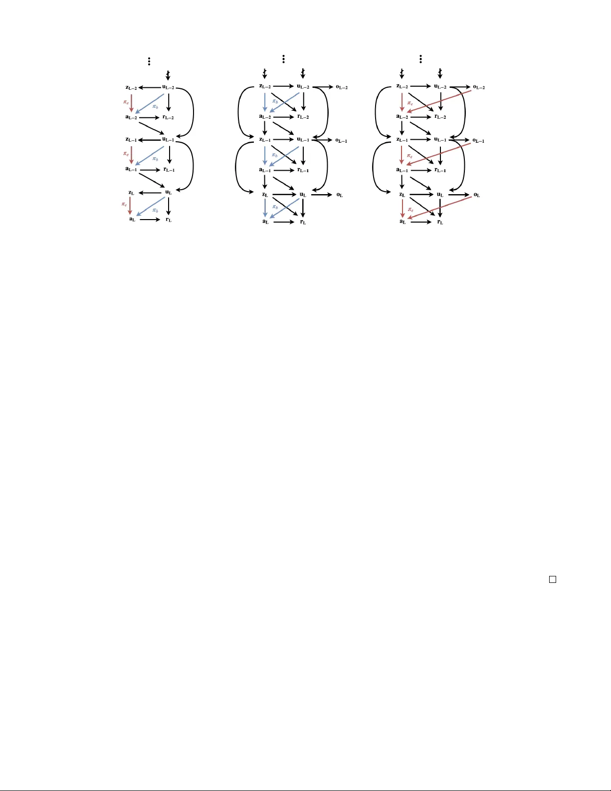
Off-P olicy Evaluation in P artially Observ able En vir onments Guy T ennenholtz T echnion Institute of T echnology Shie Mannor T echnion Institute of T echnology Uri Shalit T echnion Institute of T echnology Abstract This work studies the problem of batch of f-policy evaluation for Reinforcement Learning in partially observable environ- ments. Of f-policy e valuation under partial observability is in- herently prone to bias, with risk of arbitrarily large errors. W e define the problem of off-policy ev aluation for Partially Observable Markov Decision Processes (POMDPs) and es- tablish what we believ e is the first of f-policy e valuation result for POMDPs. In addition, we formulate a model in which ob- served and unobserved variables are decoupled into two dy- namic processes, called a Decoupled POMDP . W e show ho w off-polic y e valuation can be performed under this ne w model, mitigating estimation errors inherent to general POMDPs. W e demonstrate the pitfalls of of f-policy ev aluation in POMDPs using a well-known off-polic y method, Importance Sampling, and compare it with our result on synthetic medical data. 1 Introduction Reinforcement Learning (RL) algorithms learn to maximize rew ards by analyzing past experience in an unkno wn en- vironment (Sutton and Barto 1998). In the context of RL, off-polic y ev aluation (OPE) refers to the task of estimating the v alue of an evaluation policy without applying it, using data collected under a different behavior policy (Dann, Neu- mann, and Peters 2014), also unknown as a logging polic y . The problem of OPE has been thoroughly studied un- der fully-observable models. In this paper we e xtend and define OPE for Partially Observable Marko v Decision Pro- cesses (POMDPs). Informally , the goal of OPE in POMDPs is to ev aluate the cumulative re ward of an evaluation policy π e which is a function of observed histories, using a mea- sure over the observed variables under a behavior policy π b which is a function of an unobserved state. W e assume that we do not hav e access to the unobserved states, nor do we hav e any prior information of their model. In fact, in many cases we do not even kno w whether these states exist. These states are commonly referred to as confounding variables in the causal inference literature, whene ver the y af fect both the rew ard as well as the beha vior policy . OPE for POMDPs is highly relev ant to real-world applications in fields such as Copyright c  2020, Association for the Adv ancement of Artificial Intelligence (www .aaai.org). All rights reserv ed. healthcare, where we are trying to learn from observed poli- cies enacted by medical experts, without having full access to the information the experts ha ve in hand. A basic observation we make is that traditional meth- ods in OPE ar e not applicable to partially observable en- vironments . For this reason, we start by defining the OPE problem for POMDPs, proposing v arious OPE approaches. W e define OPE for POMDPs in Section 2. Then, in Sec- tion 3, Theorem 1 shows how past and future observations of an unobserved state can be leveraged in order to ev aluate a policy , under a non-singularity condition of certain joint probability distribution matrices. T o the best of our knowl- edge, this is the first OPE result for POMDPs. In Section 4 we build upon the results of Section 3 and propose a more in volved POMDP model: the De- coupled POMDP model. This is a class of POMDPs for which observed and unobserv ed variables are distinctly par- titioned. Decoupled POMDPs hold intrinsic adv antages ov er POMDPs for OPE. The assumptions required for OPE are more flexible than those required in POMDPs, allo wing for easier estimation (Theorem 2). In Section 5 we attempt to answer the question as to why traditional OPE methods fail when parts of the state are un- observed. W e emphasize the hardness of OPE in POMDPs through a conv entional procedure known as Importance Sampling. W e further construct an Importance Sampling variant that can be applied to POMDPs under an assumption about the rew ard structure. W e then compare this variant to the OPE result of Section 4 in a synthetic medical en viron- ment (Section 6), showing it is prone to arbitrarily large bias. Before diving into the subtleties associated with off- policy e valuation in partially observ able environments, we provide two examples in which ignoring unobserved v ari- ables can lead to erroneous conclusions about the relation between actions and their rew ards. Medical T reatment: Consider a physician monitoring a pa- tient, frequently prescribing drugs and applying treatments according to her medical state. Some of the patient’ s infor- mation observ ed by the physician may be unav ailable to us (e.g., the patient’ s socioeconomic status). A physician might tend to prescribe Drug A for her wealthier patients who can afford it. At the same time, wealthier patients tend to ha ve better outcomes re gardless of the specific drug. As we are unaware of the doctor’ s inner state for choosing this ac- tion, and have no access to the information she is using, a naiv e model would wrongly deduce that prescribing drug A is more effecti ve than it actually is. A utonomous driving: Consider teaching an autonomous vehicle to dri ve using video footage of cameras located o ver intersections. In this scenario, man y unobserved variables may be present, including: objects unseen by the camera, the dri ver’ s current mood, social cues between dri vers and pedestrians, and so on. Nai ve estimations of policies based on other driv ers’ behavior may result in catastrophic out- comes. For the purpose of this illustration, let us assume tired driv ers tend to be in volv ed in more traffic accidents than non-tired drivers. In addition, suppose non-tired driv ers tend to dri ve faster than tired driv ers. W e wish to construct a safe autonomous car based on traffic camera footage. Since the tiredness of the driv er is unobserved, a naiv e model might wrongly e v aluate a good policy as one that dri ves f ast. Understanding how to ev aluate the effects of actions in the presence of unobserved v ariables that af fect both actions and re wards is the premise of a vast array of work in the field of causal inference. Our present work owes much to ideas presented in the causal inference literature under the name of effect restoration (K uroki and Pearl 2014). In our work, we build upon a technique introduced by Miao, Geng, and Tchetgen Tchetgen (2018) on causal inference using proxy variables. In the two papers above the unobserv ed v ariable is static, and there is only one action taken. Our work deals with dynamic en vironments with sequential actions and ac- tion – hidden-state feedback loops. Surprisingly , while this is in general a harder problem, we show that these dynamics can be lev eraged to provide us with multiple noisy views of the unobserved state. Our work sits at an intersection between the fields of RL and Causal Inference. While we ha ve chosen to use termi- nology common to RL, this paper could have equiv alently been written in causal inference terminology . W e believ e it is essential to bridge the gap between these tw o fields, and include an interpretation of our results using causal infer- ence terminology in the appendix. 2 Preliminaries Partially Observ able Markov Decision Process W e consider a finite-horizon discounted P artially Observ- able Markov Decision Process (POMDP). A POMDP is defined as the 5-tuple ( U , A , Z , P , O, r, γ ) (Puterman 1994), where U is a finite state space, A is a finite action space, Z is a finite observation space, P : U × U × A 7→ [0 , 1] is a transition kernel, O : U × Z 7→ [0 , 1] is the observation function, where O ( u, z ) denotes the probability P ( z | u ) of percei ving observ a- tion z when arriving in state u , r : U × A → [0 , 1] is a re ward function, and γ ∈ (0 , 1) is the discount factor . A diagram of the causal structure of POMDPs is depicted in Figure 1a. A POMDP assumes that at an y time step the en vironment is in a state u ∈ U , an agent takes an action a ∈ A and re- ceiv es a re ward r ( u, a ) from the en vironment as a result of this action. At any time t , the agent will hav e chosen actions and recei ved re wards for each of the t time steps prior to the current one. The agent’ s observable history at time t is de- fined by h o t = ( z 0 , a 0 , . . . , z t − 1 , a t − 1 , z t ) . W e denote the space of observable histories at time t by H o t . W e consider trajectories and observ able trajectories. A trajectory of length t is defined by the sequence τ = ( u 0 , z 0 , a 0 , . . . , u t , z t , a t ) . Similarly , an observable trajectory of length t is defined by the sequence τ o = ( z 0 , a 0 , . . . , z t − 1 , a t − 1 , z t , a t ) . W e denote the space of tra- jectories and observ able trajectories of length t by T t and T o t , respectiv ely . Finally , a policy π is any stochastic, time- dependent 1 mapping from a measurable set X t ⊂ T t to the set of probability measures on the Borel sets of A , denoted by B ( A ) . For any time t , and trajectory τ ∈ T t , we define the cumu- lativ e reward R t ( τ ) = t X k =0 γ k r ( u k , a k ) . The abov e is also kno wn as the discounted return. Given any policy π and initial distrib ution ov er states U , denoted by ν 0 , we define the expected discounted return at time L by v L ( π ; ν 0 ) = E ( R L ( τ ) | u 0 ∼ ν 0 , τ ∼ π ) . When clear from context, we will assume ν 0 and L are known and fix ed and simply write v ( π ) . Policy Ev aluation Off-polic y e valuation (OPE) considers two types of policies: a behavior policy and an e valuation policy , as defined belo w . Definition 1 (behavior and e valuation policies) . A behavior policy , denoted by π ( t ) b , is a stochastic, time- dependent mapping fr om states U to B ( A ) . 2 An evaluation policy , denoted by π ( t ) e , is a stochastic, time- dependent mapping fr om observable histories H o t to B ( A ) . For any time step t and policy π let P π ( · ) be the measure ov er observable trajectories H o t , induced by polic y π . W e will denote this measure by P b , P e , whene ver π is a behavior or ev aluation policy , respectiv ely . W e are now ready to define off-polic y ev aluation in POMDPs: The goal of off-policy evaluation in POMDPs is to evaluate v L ( π e ) using the measure P b ( · ) over ob- servable trajectories T o L and the given policy π e . This corresponds to the scenario in which data comes from a system which records an agent taking actions based on her own information sources ( u ), and we w ant to ev aluate a pol- icy π e which we learn based only on information a vailable to the learning system ( τ o ). 1 For brevity we sometimes denote policies by π , though they may depend on time such that π = π ( t ) . 2 W e consider behavior policies to be functions of unobserved states. This assumption is common in MDPs in which the state is observed, as it is kno wn that there exists a stationary optimal policy that is optimal (Romanovskii 1965). In addition, the unobserved state is assumed to contain all required information for an agent to make an optimal decision. V ector Notations Let x, y , z be random variables accepting v alues in { x 1 , . . . , x n 1 } , { y 1 , . . . , y n 2 } , { z 1 , . . . , z n 3 } , respectively , and let F be a filtration that includes all information: states, ob- servations, actions, and re wards. W e denote by P ( X | y, F ) the n 1 × 1 column vector with elements ( P ( X | y , F )) i = P ( x i | y , F ) . Similarly we denote by P ( x | Y , F ) the 1 × n 2 row vector with elements ( P ( x | Y , F ) i = P ( x | y i , F ) . Note that P ( x | Y , F ) P ( Y |F ) = P ( x |F ) . Finally , let P ( X | Y , F ) be the n 1 × n 2 matrix with elements ( P ( X | Y , F )) ij = P ( x i | y j , F ) . Note that if x is independent of z giv en y then we hav e the matrix equality P ( X | Y , F ) P ( Y | Z, F ) = P ( X | Z, F ) . W e will sometimes only consider subsets of the abo ve matrices. For any index sets I ⊂ { 1 , . . . n 1 } , J ⊂ { 1 , . . . n 2 } let P ( I ,J ) ( X | Y , F ) be the matrix with elements  P ( I ,J ) ( X | Y , F )  ij = P ( x I i | y J j , F ) . 3 Policy Ev aluation for POMDPs In this section we sho w how past and future observations can be leveraged in order to create an unbiased e v aluation of π e under specific in vertibility conditions. It is a generaliza- tion of the bandit-type result presented in Miao, Geng, and Tchetgen Tchetgen (2018), where causal effects are inferred in the presence of an unobserved discrete confounder , pro- vided one has two conditionally independent vie ws of the confounder which are non-degenerate (i.e., the conditional probability matrices are inv ertible). W e show how time dy- namics readily give us these two conditionally independent views - using the past and future observations as two vie ws of the unobserved state. For an y τ o = ( z 0 , a 0 , . . . , z t , a t ) ∈ T o t we define the general- ized weight matrices W i ( τ o ) = P b ( Z i | a i , Z i − 1 ) − 1 P b ( Z i , z i − 1 | a i − 1 , Z i − 2 ) for i ≥ 1 , and W 0 ( τ o ) = P b ( Z 0 | a 0 , Z − 1 ) − 1 P b ( Z 0 ) . Here, we assume there exists an observation of some time step before initial ev aluation (i.e., t < 0 ), which we denote by z − 1 . Alternati vely , z − 1 may be an additional observ ation that is independent of z 0 and a 0 giv en u 0 . Note that the matrices W i can be estimated from the observed trajectories of the behavior distrib ution. W e then have the follo wing result. Theorem 1 (POMDP Evaluation) . Assume |Z | ≥ |U | and that P b ( Z i | a i , Z i − 1 ) ar e in vertible for all i and all a i ∈ A . F or any τ o ∈ T o t denote Π e ( τ o ) = t Y i =0 π ( i ) e ( a i | h o i ) , Ω( τ o ) = t Y i =0 W t − i ( τ o ) . Then P e ( r t ) = X τ o ∈T o t Π e ( τ o ) P b ( r t , z t | a t , Z t − 1 )Ω( τ o ) . Pr oof. See Appendix. Having ev aluated P e ( r t ) for all 0 ≤ t ≤ L suf fices in or- der to ev aluate v ( π e ) . Theorem 1 lets us ev aluate v ( π e ) with- out access to the unknown states u i . It uses past and future observations z t and z t − 1 as proxies of the unknown state. Its main assumptions are that the conditional distribution matrices P b ( Z i | a i , Z i − 1 ) and P b ( U i | a i , Z i − 1 ) are in vertible. In other words, it is assumed that enough information is trans- ferred from states to observations between time steps. Con- sider for example the case where U i and Z i are both binary , then a sufficient condition for in vertibility to hold is to have p ( z i = 1 | z i − 1 = 1 , a i ) 6 = p ( z i = 1 | z i − 1 = 0 , a i ) for all v alues of a i . A trivial case in which this assumption does not hold is when { u i } 0 ≤ i ≤ L are i.i.d. In such a scenario, the obser- vations z i , z i − 1 do not contain enough useful information of the unobserved state u i , and additional independent obser - vations of u i are needed. In the next section we will sho w how this assumption can be greatly relax ed under a decou- pled POMDP model. P articularly , in the next section we will devise an alternati ve model for partial observ ability , and an- alyze its superiority ov er POMDPs in the context of OPE. 4 Decoupled POMDPs Theorem 1 provides an exact e v aluation of π e . Ho we ver it assumes non-singularity of several large stochastic matrices. While such random matrices are likely to be in vertible (see e.g., Bordenave, Caputo, and Chafa ¨ ı (2012) Thm 1.4), es- timating their inv erses from behavior data can lead to large approximation errors or require very large sample sizes. This is due to the structure of POMDPs, which is confined to a causal structure in which unobserved states form observ a- tions. This restriction is present ev en when O ( u, z ) is a de- terministic measure. In many settings, one may detach the effect of unobserv ed and observed variables. In this section, we define a Decoupled Partially Observable Markov Deci- sion Process (Decoupled POMDP), in which the state space is decoupled into unobserved and observ ed v ariables. Informally , in Decoupled POMDPs the state space is fac- tored into observed and unobserved states. Both the ob- served and unobserved states follow Markov transitions. In addition, unobserv ed states emit independent observ ations. As we will show , Decoupled POMDPs are more appropriate for OPE under partial observ ability . Contrary to Theorem 1, Decoupled POMDPs use matrices that scale with the support of the unobserved variables, which, as they are decoupled from observed v ariables, are of much smaller cardinality . Definition 2. W e define a finite-horizon discounted Decou- pled P artially Observable Marko v Decision Process (De- coupled POMDP) as the tuple ( U , Z , O , A , P , P O , r, γ ) , wher e Z and U consist of an observed and unobserved finite state space, respectively . A is the action space, O is the indepen- dent observation space, P : Z × U × Z × U × A 7→ [0 , 1] is the transition kernel, wher e P ( z 0 , u 0 | z , u, a ) is the pr obability of transitioning to state ( z 0 , u 0 ) when visiting state ( z , u ) and taking action a , P O : U × O 7→ [0 , 1] is the independent obser- vation function, where P O ( o | u ) is the pr obability of r eceiving observation o when arrive at state u , r : U × Z × A → [0 , 1] is a r ewar d function, and γ ∈ (0 , 1) is the discount factor . A Decoupled POMDP assumes that at an y time step the en vironment is in a state ( u, z ) ∈ U × Z , an agent takes an action a ∈ A and recei ves a reward r ( u, z , a ) from the en vironment. The agent’ s observ able history is defined by (a) POMDP (b) Decoupled POMDP Figure 1: A causal diagram of a POMDP (a) and a Decoupled POMDP (b). In Decoupled POMDPs, observed and unobserved states are separated into two distinct processes, with a coupling between them at each time step. Diagrams depicts the causal dependence of a behavior policy and e valuation policies. While ev aluation policies are depicted to depend on the current observation alone, the y can depend on any observable history h o t . h o t = ( z 0 , o 0 , a 0 , . . . , z t − 1 , o t − 1 , a t − 1 , z t , o t ) . W ith abuse of no- tations we denote the space of observable histories at time t by H o t . W e similarly define trajectories and observable tra- jectories of length t by τ = ( u 0 , z 0 , o 0 , a 0 , . . . , u t , z t , o t , a t ) and τ o = ( z 0 , o 0 , a 0 , . . . , z t , o t , a t ) , respecti vely . W ith abuse of no- tations, we denote the space of trajectories and observable trajectories of length t by T t and T o t , respecti vely . In Fig- ure 1(b) we give an example of a Decoupled POMDP (used in Theorem 2) for which z i causes u i . Decoupled POMDPs hold the same expressiv e power and generality of POMDPs. T o see this, one may remove the observed state space Z to recover the original POMDP model. Nevertheless, as we will see in Theorem 2, Decou- pled POMDPs also let us leverage their structure in order to achiev e tighter results. Similar to POMDPs, OPE for Decou- pled POMDPs considers behavior and e valuation policies. Definition 3 (behavior and e valuation policies) . A behavior policy , denoted by π ( t ) b , is a stochastic, time- dependent mapping fr om states U × Z to B ( A ) . An evaluation policy , denoted by π ( t ) e , is a stochastic, time- dependent mapping fr om observable histories H o t to B ( A ) . The goal of OPE for Decoupled POMDPs is defined sim- ilarly as general POMDPs. Decoupled POMDPs allo w us to model en vironments in which observ ations are not con- tained in the unknown state. They are decoupled by a Marko- vian processes which gov erns both observed and unobserved variables. In what follo ws, we will show how this property can be lev eraged for ev aluating a desired policy . Policy Ev aluation for Decoupled POMDPs For all i , let K i ⊂ { 1 , . . . , |O |} , J i ⊂ { 1 , . . . , |Z |} such that | K i | = | J i | = | U | . Similar to before, for any τ o ∈ T o t , we de- fine the generalized weight matrices G i ( τ o ) = P b ( K i ,J i − 1 ) ( O i | z i , a i , Z i − 1 ) − 1 × × P b ( K i ,J i − 2 ) ( O i , o i − 1 , z i | z i − 1 , a i − 1 , Z i − 2 ) , for i ≥ 1 and G 0 ( τ o ) = P b ( K 0 ,J − 1 ) ( O 0 | z 0 , a 0 , Z − 1 ) − 1 P b K 0 ( O 0 | z 0 ) P b ( z 0 ) . W e then hav e the follo wing result. Theorem 2 (Decoupled POMDP Evaluation) . Assume |Z | , |O| ≥ |U | and that there exist index sets K i , J i such that | K i | = | J i | = |U | and P b ( K i ,J i − 1 ) ( O i | a i , z i , Z i − 1 ) ar e in vertible ∀ i, a i , z i ∈ A × Z . In addition assume that z i − 1 is independent of u i +1 given z i +1 , a i , u i , ∀ i under P b . F or any τ o ∈ T o t , denote by Π e ( τ o ) = t Y i =0 π ( i ) e ( a i | h o i ) , Ω( τ o ) = t Y i =0 G t − i ( τ o ) . Then P π ( r t ) = X τ o ∈T o t Π e ( τ o ) P b K t − 1 ( r t , o t | z t , a t , Z t − 1 )Ω( τ o ) . Pr oof. See Appendix. Approximating Theorem 2’ s result under finite datasets is more robust than Theorem 1. For one, the matrices are of size |U | , which can be much smaller than |Z | + |U | . In ad- dition, and contrary to Theorem 1, the result holds for any index set J i , K i ⊂ [ |Z | ] of cardinality |U | . W e can thus choose any of  |Z | |U |  possible subsets from which to approximate the matrices G i ( τ ) . This enables us to choose indices for solu- tions with desired properties (e.g., small condition numbers of the matrices). W e may also construct an estimator based on a majority vote of the separate estimators. Finally , we note that solving for G i ( τ ) for any J i , K i can be done using least squares regression. Up to this point we have shown ho w the task of OPE can be carried out in two settings: general POMDPs and Decou- pled POMDPs. The results in Theorems 1 and 2 depend on full trajectories, which we believ e are a product of the high complexity inherent to the problem of OPE with unobserv- able states. In the next section, we demonstrate the hardness inherent to OPE in these settings through an alternati ve OPE method - a v ariant of an Importance Sampling method (Pre- cup 2000). W e then experiment and compare these different OPE techniques on a synthetic medical en vironment. 5 Importance Sampling and its Limitations in Partially Observ able En vironments In previous sections we presented OPE in partially observ- able en vironments, and provided, for what we believe is the first time, techniques of exact e valuation. A reader famil- iar with OPE in fully-observ able environments might ask, why do new techniques need to be established and where do traditional methods fail? T o answer this question, in this section we demonstrate the bias that may arise under the use of long-established OPE methods. More specifically , we demonstrate the use of a well-kno wn approach, Importance Sampling (IS): a reweighting of rew ards generated by the be- havior policy , π b , such that they are equi valent to unbiased rew ards from an ev aluation policy π e . Let us be gin by defining the IS procedure for POMDPs. Suppose we are gi ven a trajectory τ ∈ T t . W e can express P e ( τ ) using P b ( τ ) as P e ( τ ) = P e ( u 0 , z 0 , a 0 , . . . , u t , z t , a t ) = ν 0 ( u 0 ) t − 1 Y i =0 P b ( u i +1 | u i , a i ) t Y i =0 P b ( z i | u i ) π ( i ) e ( a i | h o i ) = P b ( τ ) t Y i =0 π ( i ) e ( a i | h o i ) π ( i ) b ( a i | u i ) . W e refer to w i = π ( i ) e ( a i | h o i ) π ( i ) b ( a i | u i ) as the importance weights. The importance weights allow us to e v aluate v ( π e ) using the data generating process P b ( · ) as IS ( π e , w ) := E R L ( τ ) L Y i =0 w i      τ ∼ π b , u 0 ∼ ν 0 ! . (1) Note that v ( π e ) = IS ( π e , w ) . Unfortunately , the above re- quires the use of π ( i ) b ( a i | u i ) , which are unkno wn and can- not be estimated from data, as u i are unobserved under the POMDP model. Sufficient Condition f or Importance Sampling As Equation (1) does not resolve the off-polic y problem, it remains an open question whether an IS procedure can be used in general POMDPs. Here, we gi ve suf ficient con- ditions for which a v ariant of IS can properly ev aluate π e . More specifically , we assume a POMDP which satisfies the following condition. Figure 2: An example of a POMDP with 6 states and 2 ob- servations for which importance sampling with importance weights w i = π ( i ) e ( a i | h o i ) P b ( a i | h o i ) is biased. Numbers on arrows corre- spond to probabilities. Arrows marked by a 0 , a 1 correspond to re wards or transitions of these actions. Re wards depend on values of α > 0 . Initial state distribution is ν 0 = ( 1 2 , 1 2 ) . Assumption 1 (Sufficient Condition for IS) . ∃ f L : T o L 7→ R s.t. ∀ τ ∈ T L , R L ( τ ) = f L ( τ o ) and ∀ 0 ≤ i ≤ L − 1 , τ o i ∈ T o i , z i +1 ∈ Z , P b ( z i +1 | τ o i ) = P e ( z i +1 | τ o i ) . In other words, this assumption states that the observed trajectory at time L is a suf ficient statistic of the true reward, and τ o i is a suf ficient statistic of the state u i . Under Assump- tion 1 we can construct an IS variant as follo ws. Gi ven a trajectory τ ∈ T L we hav e that v ( π e ) = X τ ∈T L R ( τ ) P e ( τ ) = X u 0 ,...,u L X τ o ∈T o L f L ( τ o ) P e ( τ o , u 0 , . . . , u L ) = X τ o ∈T o L f L ( τ o ) P e ( τ o ) . W e can express P e ( τ o ) using P b ( τ o ) for any τ o ∈ T o L as P e ( τ o ) = P e ( z 0 , a 0 , . . . , z t , a t ) = P b ( z 0 ) L − 1 Y i =0 P b ( z i +1 | τ o i ) L Y i =0 π ( i ) e ( a i | h o i ) = P b ( τ o ) L Y i =0 π ( i ) e ( a i | h o i ) P b ( a i | h o i ) . W e can thus ev aluate v ( π e ) using Equation (1) and impor - tance weights w i = π ( i ) e ( a i | h o i ) P b ( a i | h o i ) . While this estimate seems simple and intuitiv e, as we demonstrate next, arbitrarily large e valuation errors can occur using the abov e IS weights when Assumption 1 does not hold. Importance Sampling Error in POMDPs In general POMDPs, if Assumption 1 does not hold, using the importance weights w i = π ( i ) e ( a i | h o i ) P b ( a i | h o i ) can result in large errors in the e valuation of π e . This error is demonstrated by an example giv en in Figure 2. In this example, we Figure 3: Comparison of cumulativ e rew ard approximation on three distinct synthetic environments. π b (green, triangles) and π e (red, circles) plots depict the true cumulati ve re wards of the behavior and e valuation policies, respecti vely . Ideally we would want the black “Theorem 2” curve and the blue IS curv e to match the red curve of the true rew ard. assume an initial state distribution ν 0 = ( 1 2 , 1 2 ) . Gi ven a behavior policy π b ( a i | u ( j ) k ) = ( 2 3 i ⊕ j = 0 1 3 i ⊕ j = 1 for all k , and a stationary ev aluation policy π e ( a i | z j ) = ( 2 3 i ⊕ j = 0 1 3 i ⊕ j = 1 , we hav e that v ( π b ) ≈ 0 . 72 α + 0 . 26 γ and v ( π e ) ≈ − 0 . 01 α + 0 . 14 γ . Howe ver , using w i = π e ( a i | z i ) P b ( a i | h o i ) , IS e valuation yields IS ( π e , w ) ≈ 0 . 62 α + 0 . 34 γ . This amounts to an error of 0 . 63 α + 0 . 2 γ between the true polic y e valuation and its im- portance sampling e valuation, which can be arbitrarily large. As an example, for α = 0 . 8 γ we get that v ( π b ) = IS ( π e , w ) . Particularly , IS ( π e , w ) > v ( π b ) for α > 0 . 8 . This is contrary to the fact that v ( π b ) > v ( π e ) for all values of α > 0 . Unlike the in vertibility assumptions of Theorems 1 and 2, Assumption 1 is a strong assumption, that is unlikely to hold for almost any POMDP . At this point it is unclear if a more lenient assumption can assure an unbiased IS estimator for POMDPs, and we leav e this as an open research question for future work. In the next section, we experiment with the results of Theorem 2 and the IS variant constructed in this section on a finite-sample dataset generated by a synthetic medical en vironment. 6 Experiments The medical domain is known to be prone to many unob- served factors af fecting both actions and rew ards (Gottes- man et al. 2018). As such, OPE in these domains requires adaptation to partially observable settings. In our experi- ments we construct a synthetic medical environment using a Decoupled POMDP model, as described next. W e denote σ ( x ) = 1 1+ e − x . The en vironment consists of a patient’ s (observed) medical state z . Here z changes accord- ing to the taken action by P ( z 0 | z , a ) ∝ σ ( c > z,z 0 ,a φ z ( z )) , where c z,z 0 ,a are gi ven weights, and φ z ( z ) are the state features. W e assume there exist unobserved variables u = ( u mood , u look ) re- lating to the doctors current mood, and how “good” the pa- tient looks to her, respectively . In other words, we assume the doctor has an inner subjectiv e ranking of the patient’ s look. Observation of the doctor’ s mood and inner ranking are modeled by P ( o | u ) ∝ σ ( c > u,o φ u ( u )) , where c u,o are giv en weights, and φ u ( u ) are the unobserved state features. Such observations could be based on the doctor’ s te xtual notes. Such notes, when processed through state of the art senti- ment analysis algorithms (Qian et al. 2016) act as proxies to the doctor’ s mood and subjectiv e assessment of the patient. W e model the doctor’ s mood changes according to the doctor’ s current mood, patient’ s look, and taken action P ( u 0 mood | u, a ) ∝ σ ( c > u,a,u 0 mood φ mood ( u )) . Finally , the doctor’ s inner ranking of the patient’ s look is de- pendent on the patient’ s state z and look u look by P ( u 0 look | z 0 , u look ) ∝ σ ( c > z 0 ,u look ,u 0 look ( φ look ( u look ) , φ z ( z ))) . W e assume data generated by a confounded reward func- tion and behavior polic y r ( u, z , a ) ∝ σ ((1 − α )( c r z,a ) > φ z ( z ) + α ( c r u,a ) > φ u ( u )) , π b ( a | u, z ) ∝ σ ((1 − α )( c b z,a ) > φ z ( z ) + α ( c b u,a ) > φ u ( u )) . Here α ∈ [0 , 1] is a parameter which controls the “level of confoundedness”. In other words, α is a measure of the in- tensity in which π b and r depend on the uno bserv ed state u , with α = 0 corresponding to no unobserved confounding. The spaces Z , U , and O were composed of two binary features each. W e run the e xperiment in three en vironments, corresponding to dif ferent settings of the vectors c meant to illustrate different behaviors of our methods. T en million tra- jectories were sampled from the policy π b ov er a horizon of 4 time steps for each en vironment. Figure 3 depicts the cumu- lativ e re ward of π e , π b , and their corresponding estimates ac- cording to Theorem 2 and the IS weights w k i = π ( i ) e ( a i | h o i ) P b ( a i | h o i ) , for different v alues of α . En vironment 1 illustrates a typical result from the genera- tiv e process abo ve, where the vectors c were sampled from a Gaussian. It is clear that IS estimates increase in bias with α , whereas Theorem 2’ s estimate remains unchanged. More- ov er , for values of α > 0 . 3 , IS suggests that π e is superior to π b . This implies that potentially arbitrarily bad policies could be learned by an of f-policy RL algorithm. Environ- ments 2 and 3 are atypical, and were found through delib- erate search, to illustrate situations in which our estimation procedure does not clearly outperform IS. In Environment 2, for large v alues of α , variance increases, due to near non- in vertibility of the conditional probability matrices. In En vi- ronment 3, despite confounding, IS remains unbiased. 7 Related W ork POMDPs: Uncertainty is a key feature in real world appli- cations. POMDPs pro vide a principled general framework for planning under uncertainty (Spaan 2012; Williams and Y oung 2007). POMDPs model aspects such as the stochastic effects of actions, incomplete information and noisy obser- vations over the en vironment. POMDPs are kno wn to be no- toriously hard to approximate (Madani, Hanks, and Condon 1999; Papadimitriou and Tsitsiklis 1987). Their intractabil- ity is mainly due to the “curse of dimensionality” for which complexity grows exponentially with the cardinality of the unobserved state space. As this work considers offline ev al- uation under uncertainty , the unobserv ed state is treated as a confounding element for policy e valuation. T o the best of our knowledge our work provides the first OPE results for POMDPs. Nevertheless, there has been considerable work on learning in POMDPs, where, simi- lar to our setting, the agent does not gain access to the POMDP model. Even-Dar , Kakade, and Mansour (2005) implement an approximate reset strategy based on a ran- dom walk of the agent, effecti vely resetting the agent’ s be- lief state. Hausknecht and Stone (2015) tackle the learning problem by adding recurrenc y to Deep Q-Learning, allow- ing the Q-network to estimate the underlying system state, narrowing the gap between Q θ ( o, a ) and Q θ ( u, a ) . Neverthe- less, w ork on learning in POMDPs greatly differs from OPE for POMDPs, as the former offer online solutions based on interactiv e en vironments, whereas the latter uses batch data generated by an unknown and unr egulated behavior polic y . Off-Policy Evaluation (OPE): Contemporary OPE meth- ods can be partitioned into three classes: (1) direct methods (DM) (Precup 2000; Munos et al. 2016; Le, V oloshin, and Y ue 2019; Jiang and Li 2015), which aim to fit the v alue of a policy directly , (2) inv erse propensity score (IPS) methods, also known as importance sampling (IS) methods (Liu et al. 2018; Dud ´ ık, Langford, and Li 2011; Jiang and Li 2015), and (3) Doubly-Rob ust methods (DRM) (Jiang and Li 2015; Thomas and Brunskill 2016; Kallus and Uehara 2019), which combine IS methods with an estimate of the action- value function, typically supplied by a DM. These algo- rithms were designed for bandits, and later generalized to RL. Nevertheless, existing methods assume full observ abil- ity of the underlying state. They become dubious when part of the data generating process is unobserved or unkno wn. Causal Infer ence: A major focus of work in causal infer - ence is how to estimate, in an offline model, the ef fects of actions without fully observing the cov ariates which lead to the action (Pearl 2009; Spirtes et al. 2000). Much of the work in this field focuses on static settings, with some more re- cent work also tackling the bandit setting (Bareinboim, For - ney , and Pearl 2015; Forney , Pearl, and Bareinboim 2017; Ramoly , Bouzeghoub, and Finance 2017; Sen et al. 2016). Sufficient “sequential ignorability” conditions (no hidden confounding) and methods for OPE of causal ef fects un- der dynamic policies are giv en by (Murphy et al. 2001; Hern ´ an et al. 2006; Hern ´ an and Robins 2019). Recently , there has been growing interest in handling un- observed confounders in the context of MDPs. Zhang and Bareinboim (2016) consider a class of counterfactual poli- cies that incorporate a notion they call “intuition”, by us- ing observed actions as input to an RL agent. Their con- founding model is a special case of our proposed Decoupled POMDP model in which confounding factors are indepen- dent of each other . Lu, Sch ¨ olkopf, and Hern ´ andez-Lobato (2018) propose a latent variable model for “deconfounding reinforcement learning”. They extend the work of Louizos et al. (2017) by positing a deep latent variable model with a sin- gle unobserved confounder that governs a trajectory , deriv- ing a variational lower bound on the likelihood and training a model with v ariational inference. Their causal model does not take into account dynamics of unobserved confounders. Oberst and Sontag (2019) also look at of f-policy ev alua- tion in POMDPs, though unlike this work they assume that the unobserv ed state does not directly affect the observed behavior -policy actions. Their work focuses on counterfac- tuals: what would ha ve happened in a specific trajectory un- der a different policy , had all the other v ariables, including the random noise v ariables, been the same. This is a diffi- cult task, lying on the third rung of Pearl’ s causal hierar- chy , which we restate in the supplementary material. (Pearl 2018). Our task is on the second rung of the hierarch y: we wish to kno w the effect of intervening on the w orld and act- ing differently , using a policy π e . Oberst and Sontag (2019) therefore requires more stringent assumptions than ours on the structure of the causal model, namely an extension of outcome monotonicity . Our work specifically extends the work of Miao, Geng, and Tchetgen Tchetgen (2018), which rests on the measure- ment of tw o independent proxy variables in a bandit setting. Our results generalizes their identification strategy through the independence structure that is inherent to POMDPs and Decoupled POMDPs, where past and future are independent conditioned on the unobserved confounder at time t . 8 Conclusion and Future W ork Off-polic y e v aluation of sequential decisions is a fundamen- tally hard problem, especially when it is done under par- tial observ ability of the state. Unkno wn states produce bias through factors that af fect both observed actions and re- wards. This paper offers one approach to tackle this problem in POMDPs and Decoupled POMDPs. While the expressi veness of POMDPs is useful in many cases, it also comes with a substantial increase in com- plexity . Y et, one may not necessarily require the complete general frame work to model complex problems. This pa- per takes a step to wards an alternative model, Decoupled POMDP , for which unobserv ed factors are isolated, reduc- ing OPE complexity , while maintaining the same expressi ve power as POMDPs. W e note that Decoupled POMDPs may also benefit general purpose RL algorithms in partially ob- servable en vironments. In this work we experimented with a tabular en vironment. As future work, one may scale up to practical domains using latent space embeddings of the generalized weight matrices, as well as sophisticated sampling techniques that may re- duce variance in approximation. References Bareinboim, E.; Forney , A.; and Pearl, J. 2015. Bandits with un- observed confounders: A causal approach. In Advances in Neural Information Pr ocessing Systems , 1342–1350. Bordenav e, C.; Caputo, P .; and Chafa ¨ ı, D. 2012. Circular law theorem for random Marko v matrices. Pr obability Theory and Related F ields 152(3-4):751–779. Dann, C.; Neumann, G.; and Peters, J. 2014. Policy e v aluation with temporal differences: A survey and comparison. The Journal of Machine Learning Resear ch 15(1):809–883. Dud ´ ık, M.; Langford, J.; and Li, L. 2011. Doubly robust policy ev aluation and learning. arXiv pr eprint arXiv:1103.4601 . Even-Dar , E.; Kakade, S. M.; and Mansour , Y . 2005. Reinforce- ment learning in POMDPs without resets. In Proceedings of the 19th international joint conference on Artificial intelligence , 690– 695. Mor gan Kaufmann Publishers Inc. Forne y , A.; Pearl, J.; and Bareinboim, E. 2017. Counterfactual data-fusion for online reinforcement learners. In Pr oceedings of the 34th International Confer ence on Machine Learning-V olume 70 , 1156–1164. JMLR. or g. Gottesman, O.; Johansson, F .; Meier, J.; Dent, J.; Lee, D.; Srini- vasan, S.; Zhang, L.; Ding, Y .; W ihl, D.; Peng, X.; et al. 2018. Evaluating reinforcement learning algorithms in observational health settings. arXiv pr eprint arXiv:1805.12298 . Hausknecht, M., and Stone, P . 2015. Deep recurrent q-learning for partially observable MDPs. In 2015 AAAI F all Symposium Series . Hern ´ an, M. A., and Robins, J. M. 2019. Causal Infer ence . Chap- man & Hall/CRC. Hern ´ an, M. A.; Lanoy , E.; Costagliola, D.; and Robins, J. M. 2006. Comparison of dynamic treatment regimes via inv erse probability weighting. Basic & clinical pharmacology & toxi- cology 98(3):237–242. Jiang, N., and Li, L. 2015. Doubly robust off-polic y value ev aluation for reinforcement learning. arXiv pr eprint arXiv:1511.03722 . Kallus, N., and Uehara, M. 2019. Double reinforcement learning for efficient off-policy ev aluation in Marko v decision processes. arXiv pr eprint arXiv:1908.08526 . Kuroki, M., and Pearl, J. 2014. Measurement bias and ef fect restoration in causal inference. Biometrika 101(2):423–437. Le, H. M.; V oloshin, C.; and Y ue, Y . 2019. Batch policy learning under constraints. arXiv pr eprint arXiv:1903.08738 . Liu, Q.; Li, L.; T ang, Z.; and Zhou, D. 2018. Breaking the curse of horizon: Infinite-horizon off-polic y estimation. In Advances in Neural Information Pr ocessing Systems , 5356–5366. Louizos, C.; Shalit, U.; Mooij, J. M.; Sontag, D.; Zemel, R.; and W elling, M. 2017. Causal effect inference with deep latent- variable models. In Advances in Neural Information Pr ocessing Systems , 6446–6456. Lu, C.; Sch ¨ olkopf, B.; and Hern ´ andez-Lobato, J. M. 2018. Deconfounding reinforcement learning in observational settings. arXiv pr eprint arXiv:1812.10576 . Madani, O.; Hanks, S.; and Condon, A. 1999. On the unde- cidability of probabilistic planning and infinite-horizon partially observable Mark ov decision problems. In AAAI/IAAI , 541–548. Miao, W .; Geng, Z.; and Tchetgen Tchetgen, E. J. 2018. Identi- fying causal effects with proxy variables of an unmeasured con- founder . Biometrika 105(4):987–993. Munos, R.; Stepleton, T .; Harutyunyan, A.; and Bellemare, M. 2016. Safe and efficient off-policy reinforcement learning. In Advances in Neur al Information Pr ocessing Systems , 1054–1062. Murphy , S. A.; van der Laan, M. J.; Robins, J. M.; and Group, C. P . P . R. 2001. Marginal mean models for dynamic re gimes. Jour - nal of the American Statistical Association 96(456):1410–1423. Oberst, M., and Sontag, D. 2019. Counterfactual off-polic y evalu- ation with Gumbel-max structural causal models. In International Confer ence on Machine Learning , 4881–4890. Papadimitriou, C. H., and Tsitsiklis, J. N. 1987. The complex- ity of Markov decision processes. Mathematics of operations r e- sear ch 12(3):441–450. Pearl, J. 2009. Causality: Models, Reasoning and Inference . New Y ork, NY , USA: Cambridge Univ ersity Press, 2nd edition. Pearl, J. 2018. Theoretical impediments to machine learning with sev en sparks from the causal rev olution. arXiv preprint arXiv:1801.04016 . Peters, J.; Janzing, D.; and Sch ¨ olkopf, B. 2017. Elements of causal infer ence: foundations and learning algorithms . MIT press. Precup, D. 2000. Eligibility traces for off-policy policy e valua- tion. Computer Science Department F aculty Publication Series 80. Puterman, M. L. 1994. Markov decision processes: discrete stochastic dynamic pr ogramming . John W iley & Sons. Qian, Q.; Huang, M.; Lei, J.; and Zhu, X. 2016. Linguistically regularized LSTMs for sentiment classification. arXiv pr eprint arXiv:1611.03949 . Ramoly , N.; Bouzeghoub, A.; and Finance, B. 2017. A causal multi-armed bandit approach for domestic robots’ failure av oid- ance. In International Confer ence on Neural Information Pr o- cessing , 90–99. Springer . Romanovskii, I. 1965. Existence of an optimal stationary pol- icy in a Mark ov decision process. Theory of Probability & Its Applications 10(1):120–122. Sen, R.; Shanmugam, K.; Kocaoglu, M.; Dimakis, A. G.; and Shakkottai, S. 2016. Contextual bandits with latent confounders: An NMF approach. arXiv pr eprint arXiv:1606.00119 . Spaan, M. T . 2012. Partially observable Markov decision pro- cesses. In Reinfor cement Learning . Springer . 387–414. Spirtes, P .; Glymour , C. N.; Scheines, R.; Heckerman, D.; Meek, C.; Cooper, G.; and Richardson, T . 2000. Causation, prediction, and sear ch . MIT press. Sutton, R. S., and Barto, A. G. 1998. Reinforcement learning: An intr oduction , volume 1. MIT press Cambridge. Thomas, P ., and Brunskill, E. 2016. Data-efficient off-policy pol- icy e valuation for reinforcement learning. In International Con- fer ence on Machine Learning , 2139–2148. W illiams, J. D., and Y oung, S. 2007. Partially observable Markov decision processes for spoken dialog systems. Computer Speech & Language 21(2):393–422. Zhang, J., and Bareinboim, E. 2016. Markov decision processes with unobserved confounders: A causal approach. T echnical re- port, T echnical Report R-23, Purdue AI Lab. 9 Acknowledgments W e thank Michael Oberst, Moshe T ennenholtz, and the anony- mous revie wers for their fruitful comments that greatly improved this paper . Research was conducted under ISF grant number 1380/16. A Main Results Local Evaluation POMDPs are known to be notoriously hard to approximate (Madani, Hanks, and Condon 1999; P apadimitriou and Tsitsiklis 1987). Their intractability is mainly due to the “curse of dimensionality” for which complexity grows exponentially with the cardinality of the state space |U | . W e thus first tackle a more modest problem, that is local in time, for which complexity does not scale with history length L . Suppose we are tasked with the limited setting of ev aluating π e only for a specific point in time, while behaving the same as the behavior policy π b at all other times. For illustrati ve purposes, we will restrict ourselves to an e valuation policy which only depends on the current observ ation z (also known as a memoryless policy). This restriction will be removed in our final results and is only assumed for clarity . More specifically , given π ( t ) b : U × A 7→ [0 , 1] and π ( t ) e : Z × A 7→ [0 , 1] we define the time- dependent policy π L as π ( t ) L = ( π ( t ) e t = L π ( t ) b o.w. Our goal is to ev aluate v L ( π L ) using the measure P b ov er observ able histories. W e generalize the bandit result presented in Miao, Geng, and Tchetgen Tchetgen (2018), in which two independent proxy v ariables of a hidden variable satisfying a certain rank condition are sufficient in order to nonparametrically ev aluate π L , ev en if the observation distribution O ( z , u ) is unknown. W e first note that for all times t < L , P π L ( r t ) = P b ( r t ) , by definition. It is thus sufficient to e valuate P π L ( r L ) . W e hav e that P π L ( r L ) = X z L ,a L ,u L P π L ( r L | z L , a L , u L ) P π L ( z L , a L , u L ) = X z L ,a L ,u L P b ( r L | a L , u L ) π ( L ) e ( a L | z L ) P b ( z L | u L ) P b ( u L ) = X z L ,a L ,u L π ( L ) e ( a L | z L ) P b ( r L , z L | a L , u L ) P b ( u L ) , (2) where the last transition is due to the fact that π b does not depend on z L giv en u L . Equation (2) can be rewritten in vector form as P π L ( r L ) = X z L ,a L π ( L ) e ( a L | z L ) P b ( r L , z L | a L , U L ) P b ( U L ) . Next, note that z L − 1 is independent of r L and z L giv en u L and a L . Therefore, P b ( r L , z L | a L , U L ) P b ( U L | a L , z L − 1 ) = P b ( r L , z L | a L , z L − 1 , U L ) P b ( U L | a L , z L − 1 ) = P b ( r L , z L | a L , z L − 1 ) . As the abov e is true for all v alues of z L − 1 and assuming the matrix P b ( U L | a L , Z L − 1 ) is in vertible for all a L ∈ A , then we can write (in vector form) P b ( r L , z L | a L , U L ) = P b ( r L , z L | a L , Z L − 1 ) P b ( U L | a L , Z L − 1 ) − 1 . (3) Similarly , we have that P b ( z L | a L , U L ) P b ( U L | a L , z L − 1 ) = P b ( z L | a L , z L − 1 , U L ) P b ( U L | a L , z L − 1 ) = P b ( z L | a L , z L − 1 ) . As the abov e is true for all v alues of z L − 1 , z L and assuming the matrix P b ( Z L | a L , U L ) is in vertible for all a L ∈ A , we can write P b ( U L | a L , Z L − 1 ) = P b ( Z L | a L , U L ) − 1 P b ( Z L | a L , Z L − 1 ) . (4) Combining Equations (3) and (4) yields P b ( r L , z L | a L , U L ) = P b ( r L , z L | a L , Z L − 1 ) P b ( Z L | a L , Z L − 1 ) − 1 P b ( Z L | a L , U L ) . Finally , note that z L is independent of a L giv en u L . Hence, P b ( Z L | a L , U L ) P b ( U L ) = P b ( Z L | U L ) P b ( U L ) = P b ( Z L ) . Lastly , note that if P b ( Z L | a L , Z L − 1 ) is in vertible, then so is P b ( Z L | a L , U L ) . Denote the generalized weight vector W L ( a L ) = P b ( Z L | a L , Z L − 1 ) − 1 P b ( Z L ) , then we hav e thus proved the follo wing proposition. Proposition 1. Suppose P b ( Z L | a L , Z L − 1 ) , P b ( U L | a L , Z L − 1 ) are in vertible for all a L ∈ A , then P π L ( r L ) = X z L ,a L π ( L ) e ( a L | z L ) P b ( r L , z L | a L , Z L − 1 ) W L ( a L ) . Proposition 1 lets us ev aluate P π L ( r L ) without access to the unknown state u L . It uses past and future observations z L and z L − 1 to create an unbiased e v aluation of P π L ( r L ) . Its main assumption is that the conditional distrib ution matrices P b ( Z L | a L , Z L − 1 ) , P b ( U L | a L , Z L − 1 ) are in vertible. In other words, it is assumed that enough information is transferred from states to observ ations between time steps. A tri vial case in which this assumption does not hold is when U i are i.i.d. In such a scenario, Z L − 1 does not contain useful information in order to e valuate r L , and an additional independent observation is needed. Nev ertheless, this assumption can be greatly reduced under a decoupled POMDP model (see Section 4). At this point, we have all needed information to ev aluate v ( π L ) . The proof of Theorem 1 iterativ ely applies a similar depen- dence in order to ev aluate v ( π e ) globally for all time steps and general history dependent ev aluation policies. Proof of Theor em 1 W e start by stating two auxiliary lemmas (their proof can be found in Appendix B. Lemma 1. P e ( r t ) = X τ o ∈T o t t Y i =0 π ( i ) e ( a i | h o i )) ! P b ( r t , z t | a t , U t )   0 Y i = t − 1 P b ( U i +1 , z i | a i , U i )   P b ( U 0 ) . Lemma 2. F or all 0 ≤ i ≤ t − 1 , let x i , y i such that x i ⊥ ( u i +1 , z i ) | a i , u i and y i ⊥ x i | a i , u i and y i ⊥ ( a i , a i − 1 , x i − 1 , z i − 1 ) | u i . Assume that the matrices P b ( U i | a i , X i ) , P b ( Y i | a i , X i ) , P b ( Y i | a i , U i ) are in vertible. Then P b ( Y i | a i , U i ) P b ( U i , z i − 1 | a i − 1 , X i − 1 ) = P b ( Y i , z i − 1 | a i − 1 , X i − 1 ) . Mor eover , P b ( U i +1 , z i | a i , U i ) P b ( U i , z i − 1 | a i − 1 , U i − 1 ) = P b ( U i +1 , z i | a i , X i ) P b ( Y i | a i , X i ) − 1 P b ( Y i , z i − 1 | a i − 1 , X i − 1 ) P b ( Y i − 1 | a i − 1 , X i − 1 ) − 1 P b ( Y i − 1 | a i − 1 , U i − 1 )) . Additionally , let x t , y t such that x t ⊥ ( r t , z t ) | a t , u t and y t ⊥ x t | a t , u t and y t ⊥ ( a t , a t − 1 , x t − 1 , z t − 1 ) | u t . Assume that the matrices P b ( U t | a t , X t ) , P b ( X t | a t , U t ) , P b ( Y t | a t , X t ) are in vertible. Then P b ( r t , z t | a t , U t ) P b ( U t , z t − 1 | a t − 1 , U t − 1 ) = P b ( r t , z t | a t , X t ) P b ( Y t | a t , X t ) − 1 P b ( Y t , z t − 1 | a t − 1 , X t − 1 ) P b ( Y t − 1 | a t − 1 , X t − 1 ) − 1 P b ( Y t − 1 | a t − 1 , U t − 1 )) . W e are now ready to complete the proof of Theorem 1. Using Lemmas 1 and 2, it holds that P b ( r t , z t | a t , U t ) t − 1 Y i =0 P b ( U i +1 , z i | a i , U i ) ! P b ( U 0 ) = P b ( r t , z t | a t , X t )   0 Y i = t − 1 P b ( Y i +1 | a i +1 , X i +1 ) − 1 P b ( Y i +1 , z i | a i , X i )   P b ( Y 0 | a 0 , X 0 ) − 1 P b ( Y 0 | a 0 , U 0 ) P b ( U 0 ) . As y 0 ⊥ a 0 | u 0 P b ( Y 0 | a 0 , U 0 ) P b ( U 0 ) = P b ( Y 0 | U 0 ) P b ( U 0 ) = P b ( Y 0 ) . Hence, P e ( r t ) = X τ o ∈T o t t Y i =0 π ( i ) e ( a i | h o i )) ! P b ( r t , z t | a t , X t )   0 Y i = t − 1 P b ( Y i +1 | a i +1 , X i +1 ) − 1 P b ( Y i +1 , z i | a i , X i )   P b ( Y 0 | a 0 , X 0 ) − 1 P b ( Y 0 ) . T o complete the proof we let x i = z i − 1 for i ≥ 1 and y i = x i +1 = z i for i ≥ 0 . Then independence assumptions of Lemma 2 indeed hold. Moreov er , it is enough to assume that P b ( Z i | a i , Z i − 1 ) is in vertible for all i ≥ 1 as P b ( z i | a i , z i − 1 ) = X u i P b ( z i | a i , z i − 1 , u i ) P b ( u i | z i − 1 , a i ) . Or in vector notation P b ( Z i | a i , Z i − 1 ) = P b ( Z i | a i , U i ) P b ( U i | Z i − 1 , a i ) . Since P b ( Z i | a i , Z i − 1 ) is in vertible, so are P b ( U i | Z i − 1 , a i ) = P b ( U i | X i , a i ) and P b ( Z i | a i , U i ) = P b ( Y i | a i , U i ) . This completes the proof of the theorem. Proof of Theor em 2 W e start by stating two auxiliary lemmas (their proof can be found in Appendix B) Lemma 3. P e ( r t ) = X τ o ∈T o t t Y i =0 π ( i ) e ( a i | h o i )) ! P b ( r t , o t | a t , z t , U t )   0 Y i = t − 1 P b ( U i +1 , z i +1 , o i | a i , z i , U i )   P b ( U 0 | z 0 ) P b ( z 0 ) . Lemma 4. F or all 0 ≤ i ≤ t − 1 , let x i , y i such that x i is independent of ( u i +1 , o i ) given z i +1 , a i , u i , y i is in- dependent of x i given z i +1 , a i , u i , and y i is independent of a i , a i − 1 , x i − 1 , z i − 1 given u i . Assume that the matrices P b ([ n ] ,J i ) ( U i | a i , z i , X i ) , P b ( K i , [ n ]) ( Y i | a i , z i , U i ) , P b ( K i ,J i ) ( Y i | a i , z i , X i ) are in vertible. Then P b ( K i , [ n ]) ( Y i | a i , z i , U i ) P b ([ n ] ,J i − 1 ) ( U i , z i , o i − 1 | a i − 1 , z i − 1 , X i − 1 ) = P b ( K i ,J i − 1 ) ( Y i , z i , o i − 1 | a i − 1 , z i − 1 , X i − 1 ) . Mor eover , P ( U i +1 , z i +1 , o i | a i , z i , U i ) P ( U i , z i , o i − 1 | a i − 1 , z i − 1 , U i − 1 ) = P b ([ n ] ,J i ) ( U i +1 , z i +1 , o i | a i , z i , X i ) P b ( K i ,J i ) ( Y i | a i , z i , X i ) − 1 P b ( K i ,J i − 1 ) ( Y i , z i , o i − 1 | a i − 1 , z i − 1 , X i − 1 ) × P b ( K i − 1 ,J i − 1 ) ( Y i − 1 | a i − 1 , z i − 1 , X i − 1 ) − 1 P b ( K i − 1 , [ n ]) ( Y i − 1 | a i − 1 , z i − 1 , U i − 1 ) . Additionally , let x t , y t such that x t is independent of r t , z t given a t , u t , y t is independent of x t given a t , u t and independent of a t , a t − 1 , x t − 1 , z t − 1 given u t . Assume that the matrices P b ( U t | a t , X t ) , P b ( X t | a t , U t ) , P b ( Y t | a t , X t ) are in vertible. Then P ( r t , o t | a t , z t , U t ) P ( U t , z t , o t − 1 | a t − 1 , z t − 1 , U t − 1 ) = P b J t ( r t , o t | a t , z t , X t ) P b ( K t ,J t ) ( Y t | a t , z t , X t ) − 1 P b ( K t ,J t − 1 ) ( Y t , z t , o t − 1 | a t − 1 , z t − 1 , X t − 1 ) × P b ( K t − 1 ,J t − 1 ) ( Y t − 1 | a t − 1 , z t − 1 , X t − 1 ) − 1 P b ( K t − 1 , [ n ]) ( Y t − 1 | a t − 1 , z t − 1 , U t − 1 ) . W e are now ready to complete the proof of Theorem 2. Using Lemmas 4 and 3, it holds that P b ( r t , o t | a t , z t , U t )   0 Y i = t − 1 P b ( U i +1 , z i +1 , o i | a i , z i , U i )   P b ( U 0 | z 0 ) P b ( z 0 ) = P b J t ( r t , o t | a t , z t , X t )   0 Y i = t − 1 P b ( K i +1 ,J i +1 ) ( Y i +1 | a i +1 , z i +1 , X i +1 ) − 1 P b ( K i +1 ,J i ) ( Y i +1 , z i +1 , o i | a i , z i , X i )   P b ( K 0 ,J 0 ) ( Y 0 | a 0 , z 0 , X 0 ) − 1 P b ( K 0 , [ n ]) ( Y 0 | a 0 , z 0 , U 0 ) P b ( U 0 | z 0 ) P b ( z 0 ) As y 0 ⊥ a 0 ) | u 0 , z 0 P b ( K 0 , [ n ]) ( Y 0 | a 0 , z 0 , U 0 ) P b ( U 0 | z 0 ) = P b ( K 0 , [ n ]) ( Y 0 | z 0 , U 0 ) P b ( U 0 | z 0 ) = P b ( Y 0 | z 0 ) . T o complete the proof we let X i = Z i − 1 and Y i = O i for i ≥ 0 . Then independence assumptions of Lemma 4 indeed hold. Moreov er , it is enough to assume that P b ( U i | a i , Z i − 1 ) and P b ( Z i | a i , Z i − 1 ) are in vertible for all i ≥ 1 as P b ( o i | a i , z i , z i − 1 ) = X u i P b ( o i | a i , z i , z i − 1 , u i ) P b ( u i | a i , z i , z i − 1 ) . Or in vector notation P b ( K i ,J i ) ( O i | a i , z i , Z i − 1 ) = P b ( K i , [ n ]) ( O i | a i , z i , U i ) P b ([ n ] ,J i ) ( U i | a i , z i , Z i − 1 ) . Since P b ( K i ,J i ) ( O i | a i , z i , Z i − 1 ) is in vertible, so are P b ( K i , [ n ]) ( O i | a i , z i , U i ) and P b ([ n ] ,J i ) ( U i | a i , z i , Z i − 1 ) . This completes the proof of the theorem. B A uxilary Lemmas Proof of Lemma 1 Pr oof. P e ( r t ) = X τ ∈T t P e ( r t | τ ) P e ( τ ) = X τ ∈T t P b ( r t | a t , u t ) P e ( τ ) . Next we ha ve that P e ( τ ) = P e ( u 0 , z 0 , a 0 , . . . , u t , z t , a t ) = P e ( a t | u 0 , z 0 , a 0 , . . . , u t , z t ) P e ( u 0 , z 0 , a 0 , . . . , u t , z t ) = π ( t ) e ( a t | h o t ) P e ( z t | u 0 , z 0 , a 0 , . . . , u t ) P e ( u 0 , z 0 , a 0 , . . . , u t − 1 , z t − 1 , a t − 1 , u t ) = π ( t ) e ( a t | h o t ) P b ( z t | u t ) P e ( u 0 , z 0 , a 0 , . . . , u t − 1 , z t − 1 , a t − 1 , u t ) = π ( t ) e ( a t | h o t ) P b ( z t | u t ) P e ( u t | u 0 , z 0 , a 0 , . . . , u t − 1 , z t − 1 , a t − 1 ) P e ( u 0 , z 0 , a 0 , . . . , u t − 1 , z t − 1 , a t − 1 ) = π ( t ) e ( a t | h o t ) P b ( z t | u t ) P b ( u t | u t − 1 , a t − 1 ) P e ( u 0 , z 0 , a 0 , . . . , u t − 1 , z t − 1 , a t − 1 ) By backwards induction we get that P e ( τ ) = t Y i =0 π ( i ) e ( a i | h o i ) P b ( z i | u i ) ! t − 1 Y i =0 P b ( u i +1 | u i , a i ) ! ν 0 ( u 0 ) . As z i is independent of a i , a i − 1 giv en u i under measure P b , we can write P b ( r t | a t , u t ) P e ( τ ) = P b ( r t , z t | a t , u t ) t Y i =0 π ( i ) e ( a i | h o i ) ! t − 1 Y i =0 P b ( u i +1 , z i | u i , a i ) ! ν 0 ( u 0 ) , which in vector form yields P e ( r t ) = X τ o ∈T o t t Y i =0 π ( i ) e ( a i | h o i )) ! P b ( r t , z t | a t , U t ) t − 1 Y i =0 P b ( U i +1 , z i | a i , U i ) ! P b ( U 0 ) . Here, the summation has now changed to observ able trajectories. Proof of Lemma 2 W e begin by pro ving an additional auxiliary lemma. Lemma 5. Let x, y , w , u, z , a be nodes in a POMDP model such that x ⊥ ( w, z ) | a, u , and y ⊥ x | a, u . Assume in addition that the matrices P b ( U | a, X ) , P b ( Y | a, X ) , P b ( Y | a, U ) ar e invertible for all a . Then P b ( W, z | a, U ) = P b ( W, z | a, X ) P b ( Y | a, X ) − 1 P b ( Y | a, U ) . Pr oof. W e start by showing that 1. If x ⊥ ( w, z ) | a, u and if P b ( U | a, X ) is in vertible for ev ery a , then P b ( W, z | a, U ) = P b ( W, z | a, X ) P b ( U | a, X ) − 1 . 2. If x ⊥ y | a, u and if P b ( X | a, U ) is inv ertible for every a , then P b ( U | a, X ) = P b ( Y | a, U ) − 1 P b ( Y | a, X ) . W e hav e that P b ( w, z | a, U ) P b ( U | a, x ) = P b ( w, z | a, x, U ) P b ( U | a, x ) = P b ( w, z | a, x ) The abov e is true for e very { x, w } , therefore P b ( W, z | a, U ) = P b ( W, z | a, X ) P b ( U | a, X ) − 1 . (5) Similarly , for the second part, we have that P b ( y | a, U ) P b ( U | a, x ) = P b ( y | a, x, U ) P b ( U | a, x ) = P b ( y | a, x ) . The abov e is true for e very { x, y } , therefore P b ( U | a, X ) = P b ( Y | a, U ) − 1 P b ( Y | a, X ) . (6) Combining Equations (5) and (6) yields P b ( W, z | a, U ) = P b ( W, z | a, X ) P b ( Y | a, X ) − 1 P b ( Y | a, U ) . W e can now continue to pro ve Lemma 2. Pr oof of Lemma 2. Let x i , y i such that x i ⊥ ( u i +1 , z i ) | a i , u i and y i ⊥ x i | a i , u i . Assume that the matrices P b ( U i | a i , X i ) , P b ( X i | a i , U i ) , P b ( Y i | a i , X i ) , P b ( Y i | a i , U i ) are in vertible. Then, by Lemma 5 P b ( U i +1 , z i | a i , U i ) = P b ( U i +1 , z i | a i , X i ) P b ( Y i | a i , X i ) − 1 P b ( Y i | a i , U i ) . Next we wish to e valuate P b ( U i +1 , z i | a i , U i ) P b ( U i , z i − 1 | a i − 1 , U i − 1 ) = P b ( U i +1 , z i | a i , X i ) P b ( Y i | a i , X i ) − 1 P b ( Y i | a i , U i ) P b ( U i , z i − 1 | a i − 1 , X i − 1 ) P b ( Y i − 1 | a i − 1 , X i − 1 ) − 1 P b ( Y i − 1 | a i − 1 , U i − 1 )) . (7) For this, let us e valuate P b ( Y i | a i , U i ) P b ( U i , z i − 1 | a i − 1 , X i − 1 ) . Assume that y i ⊥ ( a i , a i − 1 , x i − 1 , z i − 1 ) | u i , then X u i P b ( y i | a i , u i ) P b ( u i , z i − 1 | a i − 1 , x i − 1 ) = X u i P b ( y i | a i − 1 , z i − 1 , x i − 1 , u i ) P b ( u i , z i − 1 | a i − 1 , x i − 1 ) = X u i P b ( y i | a i − 1 , z i − 1 , x i − 1 , u i ) P b ( u i | z i − 1 , a i − 1 , x i − 1 ) P b ( z i − 1 | a i − 1 , x i − 1 ) = P b ( y i | a i − 1 , z i − 1 , x i − 1 ) P b ( z i − 1 | a i − 1 , x i − 1 ) = P b ( y i , z i − 1 | a i − 1 , x i − 1 ) . Therefore P b ( Y i | a i , U i ) P b ( U i , z i − 1 | a i − 1 , X i − 1 ) = P b ( Y i , z i − 1 | a i − 1 , X i − 1 ) . This prov es the first part of the lemma. The second part immediately follo ws due to Equation (10). That is, P b ( U i +1 , z i | a i , U i ) P b ( U i , z i − 1 | a i − 1 , U i − 1 ) = P b ( U i +1 , z i | a i , X i ) P b ( Y i | a i , X i ) − 1 P b ( Y i , z i − 1 | a i − 1 , X i − 1 ) P b ( Y i − 1 | a i − 1 , X i − 1 ) − 1 P b ( Y i − 1 | a i − 1 , U i − 1 )) . As the abo ve holds for all i ≥ 1 , the proof is complete. The proof for the third part follo ws the same steps with u t +1 replaced by r t . Proof of Lemma 3 Pr oof. P e ( r t ) = X τ ∈T t P e ( r t | τ ) P e ( τ ) = X τ ∈T t P b ( r t | a t , z t , u t ) P e ( τ ) . Next we ha ve that P e ( τ ) = P e ( u 0 , z 0 , o 0 , a 0 , . . . , u t , z t , o t , a t ) = P e ( a t | u 0 , z 0 , o 0 , a 0 , . . . , u t , z t , o t ) P e ( u 0 , z 0 , o 0 , a 0 , . . . , u t , z t , o t ) = π ( t ) e ( a t | h o t ) P b ( o t | u 0 , z 0 , o 0 , a 0 , . . . , u t , z t ) P e ( u 0 , z 0 , o 0 , a 0 , . . . , u t , z t ) = π ( t ) e ( a t | h o t ) P b ( o t | u t ) P e ( u t , z t | u 0 , z 0 , o 0 , a 0 , . . . , u t − 1 , z t − 1 , o t − 1 , a t − 1 ) P e ( u 0 , z 0 , o 0 , a 0 , . . . , u t − 1 , z t − 1 , o t − 1 , a t − 1 ) = π ( t ) e ( a t | h o t ) P b ( o t | u t ) P b ( u t , z t | u t − 1 , z t − 1 , a t − 1 ) P e ( u 0 , z 0 , o 0 , a 0 , . . . , u t − 1 , z t − 1 , o t − 1 , a t − 1 ) By backwards induction we get that P e ( τ ) = t Y i =0 π ( i ) e ( a i | h o i ) P b ( o i | u i ) ! t − 1 Y i =0 P b ( u i +1 , z i +1 | u i , z i , a i ) ! P b ( u 0 | z 0 ) P b ( z 0 ) . As o i is independent of a i , z i giv en u i under measure P b , we can write P b ( r t | a t , z t , u t ) P e ( τ ) = P b ( r t , o t | a t , z t , u t ) t Y i =0 π ( i ) e ( a i | h o i ) ! t − 1 Y i =0 P b ( u i +1 , z i +1 , o i | u i , z i , a i ) ! P b ( u 0 | z 0 ) P b ( z 0 ) , which in vector form yields P e ( r t ) = X τ o ∈T o t t Y i =0 π ( i ) e ( a i | h o i )) ! P b ( r t , o t | a t , z t , U t )   0 Y i = t − 1 P b ( U i +1 , z i +1 , o i | a i , z i , U i )   P b ( U 0 | z 0 ) P b ( z 0 ) . Here, the summation has now changed to observ able trajectories. Proof of Lemma 4 The proof of this lemma is similar to that of Lemma 2 and is brought here for completeness. W e begin by proving an auxiliary lemma. Lemma 6. Let x, y , w, u, z , z 0 , o, a be nodes in a Decoupled POMDP model suc h that x ⊥ ( w, o ) | a, z , u , and y ⊥ x | a, z , u . Let I , J, K be index sets such that | I | = | J | = | K | = | U | = n . Also let [ n ] be the index set { 1 , . . . , | U |} . Assume in addition that the matrices P b [ n ] ,J ( U | a, z , X ) , P b ( K, [ n ]) ( Y | a, z , U ) , P b ( K,J ) ( Y | a, z , X ) ar e in vertible for all a, z . Then P b ( I , [ n ]) ( W, z 0 , o | a, z , U ) = P b ( I ,J ) ( W, z 0 , o | a, z , X ) P b ( K,J ) ( Y | a, z , X ) − 1 P b ( K, [ n ]) ( Y | a, z , U ) . Pr oof. W e start by showing that 1. If x ⊥ ( w, z 0 , o ) | a, z , u and if P b ([ n ] ,J ) ( U | a, z , X ) is in vertible for ev ery a, z , then P b ( I , [ n ]) ( W, z 0 , o | a, z , U ) = P b ( I ,J ) ( W, z 0 , o | a, z , X ) P b [ n ] ,J ( U | a, z , X ) − 1 . 2. If x ⊥ y | a, z , u and if P b ( J, [ n ]) ( X | a, z , U ) is in vertible for ev ery a, z , then P b ([ n ] ,J ) ( U | a, z , X ) = P b ( K, [ n ]) ( Y | a, z , U ) − 1 P b ( K,J ) ( Y | a, z , X ) . W e hav e that P b ( w, z 0 , o | a, z , U ) P b ( U | a, z , x ) = P b ( w, z 0 , o | a, z , x, U ) P b ( U | a, z , x ) = P b ( w, z 0 , o | a, z , x ) The abov e is true for e very { x, w } , therefore P b ( I , [ n ]) ( W, z 0 , o | a, z , U ) = P b ( I ,J ) ( W, z 0 , o | a, z , X ) P b ([ n ] ,J ) ( U | a, z , X ) − 1 . (8) Similarly , for the second part, we have that P b ( y | a, z , U ) P b ( U | a, z , x ) = P b ( y | a, z , x, U ) P b ( U | a, z , x ) = P b ( y | a, z , x ) . The abov e is true for e very { x, y } , therefore P b ([ n ] ,J ) ( U | a, z , X ) = P b ( K, [ n ]) ( Y | a, z , U ) − 1 P b ( K,J ) ( Y | a, z , X ) . (9) Combining Equations (8) and (9) yields P b ( I , [ n ]) ( W, z 0 , o | a, z , U ) = P b ( I ,J ) ( W, z 0 , o | a, z , X ) P b ( K,J ) ( Y | a, z , X ) − 1 P b ( K, [ n ]) ( Y | a, z , U ) . W e can now continue to pro ve Lemma 4. Pr oof of Lemma 4. Let x i , y i such that x i ⊥ ( u i +1 , o i ) | z i +1 , a i , u i and y i ⊥ x i | z i +1 , a i , u i . Assume that the matrices P b ([ n ] ,J i ) ( U i | a i , z i , X i ) , P b ( K i , [ n ]) ( Y i | a i , z i , U i ) , P b ( K i ,J i ) ( Y i | a i , z i , X i ) are in vertible. Then, by Lemma 6 P ( U i +1 , z i +1 , o i | a i , z i , U i ) = P b ([ n ] ,J i ) ( U i +1 , z i +1 , o i | a i , z i , X i ) P b ( K i ,J i ) ( Y i | a i , z i , X i ) − 1 P b ( K i , [ n ]) ( Y i | a i , z i , U i ) . Next we wish to e valuate P ( U i +1 , z i +1 , o i | a i , z i , U i ) P ( U i , z i , o i − 1 | a i − 1 , z i − 1 , U i − 1 ) = P b ([ n ] ,J i ) ( U i +1 , z i +1 , o i | a i , z i , X i ) P b ( K i ,J i ) ( Y i | a i , z i , X i ) − 1 P b ( K i , [ n ]) ( Y i | a i , z i , U i ) × P b ([ n ] ,J i − 1 ) ( U i , z i , o i − 1 | a i − 1 , z i − 1 , X i − 1 ) P b ( K i − 1 ,J i − 1 ) ( Y i − 1 | a i − 1 , z i − 1 , X i − 1 ) − 1 P b ( K i − 1 , [ n ]) ( Y i − 1 | a i − 1 , z i − 1 , U i − 1 ) . (10) For this, let us e valuate P b ( K i , [ n ]) ( Y i | a i , z i , U i ) P b ([ n ] ,J i − 1 ) ( U i , z i , o i − 1 | a i − 1 , z i − 1 , X i − 1 ) . Assume that y i ⊥ ( a i , a i − 1 , x i − 1 , z i − 1 , z i ) | u i , then X u i ∈U P b ( y i | a i , z i , u i ) P b ( u i , z i , o i − 1 | a i − 1 , z i − 1 , x i − 1 ) = X u i ∈U P b ( y i | u i , z i , o i − 1 , a i − 1 , z i − 1 , x i − 1 ) P b ( u i , z i , o i − 1 | a i − 1 , z i − 1 , x i − 1 ) = X u i ∈U P b ( y i , u i , z i , o i − 1 | a i − 1 , z i − 1 , x i − 1 ) = P b ( y i , z i , o i − 1 | a i − 1 , z i − 1 , x i − 1 ) . Therefore P b ( K i , [ n ]) ( Y i | a i , z i , U i ) P b ([ n ] ,J i − 1 ) ( U i , z i , o i − 1 | a i − 1 , z i − 1 , X i − 1 ) = P b ( K i ,J i − 1 ) ( Y i , z i , o i − 1 | a i − 1 , z i − 1 , X i − 1 ) . This prov es the first part of the lemma. The second part immediately follo ws due to Equation (10). That is, P ( U i +1 , z i +1 , o i | a i , z i , U i ) P ( U i , z i , o i − 1 | a i − 1 , z i − 1 , U i − 1 ) = P b ([ n ] ,J i ) ( U i +1 , z i +1 , o i | a i , z i , X i ) P b ( K i ,J i ) ( Y i | a i , z i , X i ) − 1 P b ( K i ,J i − 1 ) ( Y i , z i , o i − 1 | a i − 1 , z i − 1 , X i − 1 ) × P b ( K i − 1 ,J i − 1 ) ( Y i − 1 | a i − 1 , z i − 1 , X i − 1 ) − 1 P b ( K i − 1 , [ n ]) ( Y i − 1 | a i − 1 , z i − 1 , U i − 1 ) . As the abov e holds for all i ≥ 1 , the proof is complete. The proof for the third part follows the same steps with ( u t +1 , z t +1 ) replaced by r t . C Bridging the Gap between Reinf orcement Lear ning and Causal Inference This section is dev oted to addressing the definition and results of this paper in terminology common in the Causal Inference literature (Pearl 2009; Peters, Janzing, and Sch ¨ olkopf 2017). W e begin with preliminaries on Structural Causal Models and Pearl’ s Do-Calculus, and continue by defining OPE as an identification problem for Causal Inference. Finally , we show that results presented in this paper relate to the counterfactual ef fect of applying the dynamic treatment π e (Hern ´ an and Robins 2019). Preliminaries The basic semantical framew ork of our analysis relies on Structural Causal Models (Pearl 2009). Definition 4 (Structural Causal Models) . A structural causal model (SCM) M is a 4-tuple h U, V , F , P ( U ) i wher e: • U is a set of e xogenous (unobserved) variables, which ar e determined by factors outside of the model. • V is a set { V i } n i =1 of endogenous (observed) variables that ar e determined by variables in U ∪ V . • F is a set of structural functions { f i } n i =1 , wher e eac h f i is a process by which V i is assigned a value v i ← f i ( pa i , u i ) in r esponse to the curr ent values of its parents P A i ⊂ V and U i ⊆ U . • P ( U ) is a distribution over the e xogenous variables U . Consider the causal graph of Figure 1a. This causal graph corresponds to an SCM that defines a complete data-generating processes P b , which entails the observ ational distrib ution. It also defines the interventional distribution P e : under P e , the arro ws labeled π e exist and denote a functional relationship between a t and z t giv en by the e valuation policy π e , and the arro ws labeled π b do not exist. Queries are questions ask ed based on a specific SCM, and are often related to interv entions, which can be thought of as idealized experiments, or as well-defined changes in the world. Formally , interventions take the form of fixing the value of one variable in an SCM and observing the result. The do-operator is used to indicate that an experiment explicitly modified a variable. Graphically , this blocks any causal factors that would otherwise af fect that v ariable. Diagramatically , this erases all causal arrows pointing at the e xperimental variable. Definition 5 (Interventional Distrib ution) . Given an SCM, an intervention I = do  x i := ˜ f ( g P A i , ˜ U i )  corr esponds to r eplacing the structural mechanism f i ( P A i , U i ) with ˜ f i ( g P A i , U i ) . This includes the concept of atomic interventions, wher e we may write more simply do ( X i = x ) . The interventional distribution is subsumed by the counterfactual distrib ution, which asks in retrospectiv e what might hav e happened had we acted dif ferently at the specific realization. T able 1 shows the 3-layer hierarchy of Pearl (2018), together with the characteristic questions that can be answered at each level. While work such as Oberst and Sontag (2019) is centered around the counterfactual layer , this paper focuses on the interv entional layer associated with the syntactic signature of the type P ( y | do ( x ) , z ) . The do-calculus is the set of manipulations that are av ailable to transform one e xpression into another , with the general goal of transforming expressions that contain the do-operator into e xpressions that do not contain it, and which in volv e only observable quantities. Expressions that do not contain the do-operator and include only observable quantities can be estimated from observational data alone, without the need for an experimental intervention. The do-calculus includes three rules for the transformation of conditional probability e xpressions in volving the do-operator . They are stated formally below . Let x, y , z , w be nodes in an SCM G . • Rule 1 (Insertion/deletion of observations) P ( y | do ( x ) , z , w ) = P ( y | do ( x ) , w ) if y and z are d -separated by x ∪ w in G ∗ , the graph obtained from G by removing all arro ws pointing into variables in x . • Rule 2 (Action/observation exchange) P ( y | do ( x ) , do ( z ) , w ) = P ( y | do ( x ) , z , w ) if y and z are d -separated by x ∪ w in G † , the graph obtained from G by removing all arrows pointing into v ariables in x and all arrows pointing out of v ariables in z . • Rule 3 (Insertion/deletion of actions) P ( y | do ( x ) , do ( z ) , w ) = P ( y | do ( x ) , w ) if y and z are d -separated by x ∪ w in G • , the graph obtained from G by first removing all the arrows pointing into variables in x (thus creating G ∗ ) and then removing all of the arro ws pointing into variables in z that are not ancestors of any v ariable in w in G ∗ . Lev el (Symbol) T ypical Activity T ypical Questions 1. Association P ( y | x ) Seeing What is? How w ould seeing x change my belief in y? *2. Intervention P ( y | do ( x ) , z ) Doing Intervening What if? What if I do x? 3. Counterfactual P ( y x | x 0 , y 0 ) Imagining Retrospection Why? W as it x that caused y? What if I had acted differently? T able 1: The three layer causal hierarchy , as gi ven in Pearl (2018). OPE in the form we gi ve is part of the second, interventional layer . In addition to the above, letting π e be a stochastic time-dependent ev aluation policy , then under the SCM of Figure 1a we have the following lemma (we use z 0: t to denote the set { z 0 , . . . z t } ). Lemma 7. P ( x t | do ( π ) , z 0: t ) = X a 0 ,...,a t P ( x t | do ( a 0 ) , . . . , do ( a t ) , z 0: t ) t Y i =0 π ( i ) e ( a i | h o i ) . Pr oof. W e hav e that P ( x t | do ( π ) , z 0: t ) = P  x t | do  π (0) e  , . . . , do  π ( t ) e  , z 0: t  , where we recall that π ( i ) e is the (possibly time-dependent) policy at time i . It is enough to sho w that for all 0 ≤ k ≤ t P ( x t | do  π (0) e  , . . . , do  π ( t ) e  , z 0: t ) = X a 0 ,...,a k P  x t | do ( a 0 ) , . . . do ( a k ) , do  π ( k +1) e  , . . . , do  π ( t ) e  , z 0: t  k Y i =0 π ( i ) e ( a 0 | h o i ) . (11) Equation (11) follows immediately by induction o ver k , as π ( i ) e depends only on its previously observ ed history . OPE as an Identification Problem In order to define OPE as an intervention problem, we define the interv entional v alue of a policy π giv en an SCM as v do ( π ) = E ( R L ( τ ) | do ( π )) . W e are now ready to define OPE in POMDPs. Let π e , π b be ev aluation policies as defined in Definition 1. The goal of of f-policy e valuation in POMDPs is to evaluate v do ( π e ) for the SCM of F igure 1a under the data g enerating pr ocess P b . W e can now restate the results presented in the paper using the abo ve terminology . W e restate Theorem 1 and Lemma 1 below . An extension to Theorem 2 and Lemma 3 is done similarly . Theorem (POMDP Ev aluation) . Assume P b ( Z i | a i , Z i − 1 ) and P b ( U i | a i , Z i − 1 ) ar e invertible for all i and all a i ∈ A . F or any τ o ∈ T o t denote Π e ( τ o ) = t Y i =0 π ( i ) e ( a i | h o i ) , Ω( τ o ) = t Y i =0 W t − i ( τ o ) . Then P ( r t | do ( π e )) = X τ o ∈T o t Π e ( τ o ) P b ( r t , z t | a t , Z t − 1 )Ω( τ o ) . The proof of the theorem follows the same steps as in Appendix A. Nev ertheless, it requires an alternate interpretation and proof of Lemma 1, which we state and prov e formally belo w . Lemma 8. P ( r t | do ( π e )) = X τ o ∈T o t t Y i =0 π ( i ) e ( a i | h o i )) ! P b ( r t , z t | a t , U t ) t − 1 Y i =0 P b ( U i +1 , z i | a i , U i ) ! P b ( U 0 ) . Pr oof. Let π e be an ev aluation policy . P ( r t | do ( π e )) = X u 0: t P ( r t | do ( π e ) , u 0: t ) P ( u 0: t | do ( π e )) = X u 0: t P ( r t | do ( π e ) , u 0: t ) P ( u 0 | do ( π e )) t − 1 Y i =0 P ( u i +1 | do ( π e ) , u 0: i ) (12) P ( u 0 | do ( π e )) = P b ( u 0 ) = ν 0 ( u 0 ) by definition and rule 3. Next we ev aluate P ( u i +1 | do ( π e ) , u 0: i ) , using the conditional indepen- dence relations of the POMDP causal graph Figure 1(a). P ( u i +1 | do ( π e ) , u 0: i ) = = X z 0: i ∈Z i +1 P ( u i +1 | do ( π e ) , z 0: i , u 0: i ) P ( z i | do ( π e ) , z 0: i − 1 , u 0: i ) P ( z 0: i − 1 | do ( π e ) , u 0: i ) . (13) Next, by Lemma 7 and the rules of do-calculus we ha ve in the POMDP causal graph: P ( u i +1 | do ( π e ) , z 0: i , u 0: i ) = X a 0: i ∈A i +1 P ( u i +1 | do ( a 0 ) , . . . , do ( a i ) , z 0: i , u 0: i ) i Y k =0 π ( k ) e ( a k | h o k ) = ( rule 3) X a 0: i ∈A i +1 P ( u i +1 | do ( a i ) , z 0: i , u 0: i ) i Y k =0 π ( k ) e ( a k | h o k ) = X a i ∈A P ( u i +1 | do ( a i ) , z 0: i , u 0: i ) π ( i ) e ( a i | h o i ) = ( rule 1) X a i ∈A P ( u i +1 | do ( a i ) , u i ) π ( i ) e ( a i | h o i ) = ( rule 2) X a i ∈A P b ( u i +1 | a i , u i ) π ( i ) e ( a i | h o i ) . (14) Also, using the POMDP causal graph and by Lemma 7, P ( z i | do ( π e ) , z 0: i − 1 , u 0: i ) = X a 0: i − 1 ∈A i P ( z i | do ( a 0 ) , . . . , do ( a i − 1 ) , z 0: i − 1 , u 0: i ) i − 1 Y k =0 π ( k ) e ( a k | h o k ) = ( rule 3) X a 0: i − 1 ∈A i P b ( z i | z 0: i − 1 , u 0: i ) i − 1 Y k =0 π ( k ) e ( a k | h o k ) = P b ( z i | u i ) . (15) Plugging Equations (14), (15) into (13) yields P ( u i +1 | do ( π e ) , u 0: i ) = X z 0: i ∈Z i +1 P ( u i +1 | do ( π e ) , z 0: i , u 0: i ) P ( z i | do ( π e ) , z 0: i − 1 , u 0: i ) P ( z 0: i − 1 | do ( π e ) , u 0: i ) = X z 0: i ∈Z i +1 X a i ∈A P b ( u i +1 | a i , u i ) π ( i ) e ( a i | h o i ) P b ( z i | u i ) P ( z 0: i − 1 | do ( π e ) , u 0: i ) = X z i ∈Z X a i ∈A P b ( u i +1 | a i , u i ) π ( i ) e ( a i | h o i ) P b ( z i | u i ) X z 0: i − 1 ∈Z i P ( z 0: i − 1 | do ( π e ) , u 0: i ) = X z i ∈Z X a i ∈A P b ( u i +1 | a i , u i ) π ( i ) e ( a i | h o i ) P b ( z i | u i ) = X z i ∈Z X a i ∈A P b ( u i +1 | a i , z i , u i ) π ( i ) e ( a i | h o i ) P b ( z i | a i , u i ) . (16) W e continue by ev aluating P ( r t | do ( π e ) , u 0: t ) . Similar to before, P ( r t | do ( π e ) , u 0: t ) = = ( rule 1) P ( r t | do ( π e ) , u t ) = X z t ∈Z P ( r t | do ( π e ) , u t , z t ) P ( z t | do ( π e ) , u t ) = X z t ∈Z X a t ∈A P b ( r t | a t , u t ) π ( t ) e ( a t | h o t ) P b ( z t | u t ) = X z t ∈Z X a t ∈A P b ( r t | a t , z t , u t ) π ( t ) e ( a t | h o t ) P b ( z t | a t , u t ) . (17) Plugging Equations (16), (17) into Equation (12) yields P ( r t | do ( π e )) = X u 0: t P ( r t | do ( π e ) , u 0: t ) P ( u 0 | do ( π e )) t − 1 Y i =0 P ( u i +1 | do ( π e ) , u 0: i ) = X τ ∈T t P b ( r t , z t | a t , u t ) t Y i =0 π ( i ) e ( a i | h o i ) ! t − 1 Y i =0 P b ( u i +1 , z i | u i , a i ) ! ν 0 ( u 0 ) , which can be written in vector form as P ( r t | do ( π e )) = X τ o ∈T o t t Y i =0 π ( i ) e ( a i | h o i ) ! P b ( r t , z t | a t , U t ) t − 1 Y i =0 P b ( U i +1 , z i | a i , U i ) ! P b ( U 0 ) This completes the proof. A ppendix D: Experimental Details Figure 4 In our experiments we used three en vironments of dif ferent sampled v ectors. V ectors were sampled uniformly from a normal distribution. W e’ ve chosen to depict in our paper , environments that had different characteristics of our results. Nev ertheless, most sampled en vironments were unbiased for Theorem 2’ s result, and highly biased for the IS estimator . Figure 4 depicts two other environments for which IS is highly biased. W e also provide code of our experiments and medical en vironment in the supplementary material.