Revisiting the probabilistic method of record linkage

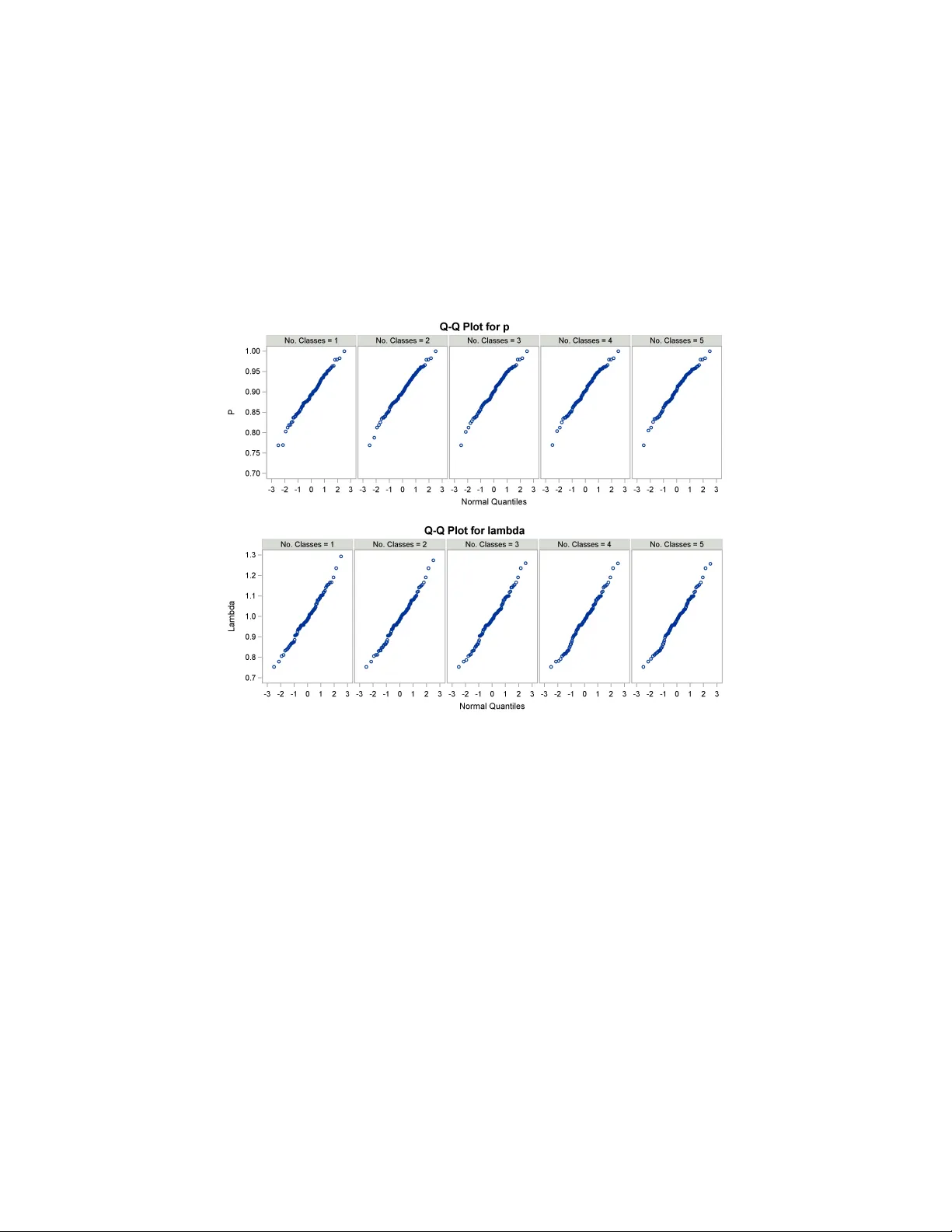
Revisiting the probabilistic metho d of record link age A. Dasylv a ∗ , A. Goussanou, D. Aja v on Statistics Canada and H. Ab ousal eh Departmen t of Mathematics and Statistics, Univ ersit y of Victoria No v em b er 6, 2019 Abstract In theory , the probabilistic link age method pro vides t w o distinct adv an tages o v er non- probabilistic methods, including minimal rates of link age error and accurate measures of these rates for data users. Ho wev er, implementations can fall short of these exp ec- tations either b ecause the conditional indep endence assumption is made, or because a mo del with interactions is used but lac ks the identiﬁcation prop ert y . In oﬃcial statistics, this is curren tly the main challenge to the automated pro duction and use of linked data. T o address this c hallenge, a new metho dology is describ ed for pr op er link age problems, where matc hed records may b e iden tiﬁed with a probability that is b ounded aw a y from zero, re gardless of the p opulation size. It mo dels the n um b er of neighb ours of a giv en record, i.e. the n um b er of resem bling records. T o b e sp eciﬁc, the prop osed mo del is a ﬁnite mixture where each component is the sum of a Bernoulli v ariable with an indep endent Poisson v ariable. It has the iden tiﬁcation property and yields solutions for man y longstanding problems, including the ev aluation of b lo ck- ing criteria and the estimation of link age errors for probabilistic or nonprobabilistic link ages, all without clerical reviews or conditional indep endence assumptions. Thus it also enables unsup ervised machine learning solutions for record link age problems. ∗ ab el.dasylv a@canada.ca 1 Keywor ds: en tit y resolution, deduplication, classiﬁcation, data in tegration, massive data sets. Disclaimer : The conten t of this article represen ts the p osition of the authors and ma y not necessarily represen t that of Statistics Canada. This article describ es theoretical approaches and do es not reﬂect curren tly implemen ted methods at Statistics Canada. 2 1 In tro duction Fift y y ears ago, F ellegi and Sunter published their landmark pap er F ellegi and Sunter ( 1969 ), where they formalized probabilistic record link age. Since then, record link age has b ecome an important to ol in oﬃcial statistics. It consists in ﬁnding records from the same individual in diﬀeren t ﬁles and diﬀers from statistic al matching D’Orazio et al. ( 2006 ); a form of imputation whic h consists in ﬁnding records from similar individuals. Record link- age is also diﬀerent from automate d c o ding , where the goal is assigning a given observ ation to a class among a ﬁxed n um b er of classes. There are coun tless competing solutions for implemen ting a record link age Christen ( 2012 ). Y et in the probabilistic metho d, errors play a central role. They include false p ositiv es and false negativ es, where a false p ositive is a link b et w een t w o unmatc hed records and a false negativ e is the absence of a link b et w een t wo matched records. In its fully automated form (i.e. with a single w eight threshold) the probabilistic metho d is simply an application of Neyman-P earson lemma Neyman and Pearson ( 1933 ). Hence it promises tw o ma jor adv antages ov er its comp etitors. The ﬁrst adv antage is a minimal type I I error for a ﬁxed t yp e I error, under the null hypothesis that tw o records are matc hed. Alternatively , the link age can minimize the type I error for a ﬁxed type I I error. The second adv an tage is the accurate estimation of both kinds of error in a fully automated manner. In practice, the promise of the probabilistic method has b een elusiv e, b ecause fulﬁlling it requires a very go o d statistical mo del for the estimation of the necessary link age parameters, including the link age weigh ts and the related thresholds. The most common mo del has b een a log- linear mixture with the assumption that the link age v ariables are conditionally indep enden t giv en a pair matc h status F ellegi and Sun ter ( 1969 ). Ho w ev er, this assumption has lead to biased estimators b ecause, quite often, it has been inconsistent with actual data. F or 3 example, when linking so cial data, giv en names and last names are not indep enden t for a giv en individual. T o o v ercome this limitation, log-linear mixtures with in teractions ha v e b een considered. Y et, these mo dels hav e b een hard to use. Indeed, in the past ﬁfty y ears, they hav e b een successfully applied without lab eled pairs (i.e. pairs that are known to b e matched or unmatched), but only in a handful of studies including that by Winkler Winkler ( 1993 ). Since log-linear mo dels with in teractions are not generally kno wn to ha ve the iden tiﬁcation prop ert y , some of them may lac k it. In suc h a model, there are simply to o man y parameters to estimate from the data at hand, no matter how large the sample. This a serious problem for analysts, who need accurate measures of the error rates Neter et al. ( 1965 ); Scheuren and Winkler ( 1993 ); Ding and Fien b erg ( 1994 ); Lahiri and Larsen ( 2005 ); Chipp erﬁeld et al. ( 2011 ); Chambers and Kim ( 2016 ); Hof and Zwinderman ( 2015 ). Besides, pro ving the iden tiﬁcation of a log-linear mixture model is a non-trivial matter, ev en when the conditional assumption is made Fien b erg et al. ( 2009 ). In this regard, ha ving few er mo del parameters than estimating equations falls short of proving the iden tiﬁcation prop ert y Fien b erg et al. ( 2009 ). Probabilistic link age suﬀers from another limitation regarding false negatives caused b y blo c king criteria. Indeed, blo c king is an essential operation when linking large ﬁles. Y et it generates false negativ es that are hard to measure giv en the sheer size of the Cartesian pro duct. Herzog et al. Herzog et al. ( 2007 ) hav e describ ed a capture-recapture technique that requires t wo conditionally independent blo c king k eys. Their metho d counts the n um- b er of matc hed pairs that agree on the ﬁrst k ey , on the second k ey and on both. In practice, applying this metho d is challenging b ecause there are usually no such k eys. Even if it were the case, the metho d requires the iden tiﬁcation of eac h matc hed pair that meets a given blo c king criterion. With large ﬁles that include millions of records, this is prohibitively 4 exp ensiv e ev en if resources for reliable clerical reviews are a v ailable. The remaining sections are organized as follo ws. Section 2 presen ts the notations and assumptions. It also introduces the crucial concepts of neighb ourho o d and pr op er link age problem. Section 3 articulates the relationship betw een the probabilistic link age parame- ters and the error rates, on one hand, and the distributional parameters for the n umber of neighbours, on the other hand. Section 4 describ es the estimation pro cedure for the distribution of the n umber of neighbours. It in v olves an Exp ectation-Maximization (E-M) pro cedure Dempster et al. ( 1977 ). Section 5 cov ers the sim ulations. Section 6 describ es the empirical study . Section 7 concludes with future w ork. All the pro ofs are found in the supplemen tary material. 2 Notation and assumptions In probabilistic record link age, statistical inference ab out link age parameters and errors is commonly based on the maximization of a lik eliho o d for a sample of record pairs Winkler ( 1988 ); Jaro ( 1989 ). Most of the time, this likelihoo d is actually a c omp osite lik eliho o d V arin et al. ( 2011 ) b ecause the pairs are correlated. In general, the choice of maxim um lik eliho o d procedures is justiﬁed b y the asymptotic prop erties of the resulting estimators when the sample size tends to inﬁnit y . In our con text, this makes sense if record link age remains a viable option even when the p opulation b ecomes arbitrarily large. This is p os- sible only if the link age v ariables pro vide more information as the p opulation gro ws, such that matched records may b e identiﬁed with a probabilit y that is b ounded a w ay from zero, regardless of the p opulation size. T o discuss pro cedures for v alid statistical inference ab out link age parameters or errors, we restrict ourselves to the class of pr op er link age problems, 5 whic h satisfy this prop ert y and include all practical situations where record link age is a viable alternativ e. Outside this class, problems are impr op er and b etter view ed as satis- tical matc hing or automated coding problems. The concept of a proper link age problem is also consisten t with the use of the Shanon entrop y ( Cov er and Thomas , 1991 , c hap. 2.1) to measure the discriminating p ow er of link age v ariables and to decide if tw o ﬁles could b e link ed ( Statistics Canada , 2017 , chap. 4.2). Discussing what might happ en to a link age when the p opulation size grows is also crucial for the future of oﬃcial statistics. Indeed, man y national statistical oﬃces hav e recen tly em bark ed on the construction of an infrastucture of link ed statistical registers W allgren and W allgren ( 2014 ), through multiple link ages, including man y without a unique iden tiﬁer. This discussion can provide imp ortant insigh ts into curren t design decisions that will ha v e a ma jor impact on the production of oﬃcial statistics and public p olicy for decades to come. W e next give some notation and a mathematical deﬁnition of what constitutes a prop er link age problem, including imp ortan t consequences of this deﬁnition. Notation : With few exceptions, we denote a scalar b y a low er-case letter and a v ector or matrix b y a b oldface low er-case letter. This conv en tion also applies to a random v ariable, v ector or matrix. In general, the same symbol is used for a random v ariable (vector or matrix) and for a sp eciﬁc v alue of this v ariable (v ector or matrix). How ev er, when needed for clarity , an upp er-case letter is used for a random v ariable (v ector or matrix) while the corresp onding low er-case letter is used for a sp eciﬁc v alue. In general, a scalar function is denoted b y a low er-case letter while a v ector-v alued (or matrix-v alued) function is denoted b y a b oldface lo w er-case letter. F or a t wice diﬀeren tiable scalar m ultiv ariate function f ( . ) of ψ = ( ψ 1 , . . . , ψ q ) ∈ I R q , w e let  ∂ /∂ ψ >  f = ∂ f /∂ ψ > = [ ∂ f /∂ ψ 1 . . . ∂ f /∂ ψ q ] Schott ( 1997 ). W e also denote the Hessian matrix of f ( . ) b y  ∂ 2 /∂ ψ ∂ ψ >  f = [ ∂ 2 f /∂ ψ r ∂ ψ s ] 1 ≤ r,s ≤ q . 6 F or our sp eciﬁc problem, consider a large p opulation of N indep endent and iden tically dis- tributed individuals. Individual i is asso ciated with record v i in register A and record v 0 π ( i ) in register B , where v i and v 0 π ( i ) b elong to a set V N of (p ossibly high-dimensional) categor- ical vectors and π ( . ) is an unknown random p erm utation of { 1 , . . . , N } . The p ermutation is assumed to b e uniformly random independently of the records, i.e. P  π ( . )     v i , v 0 π ( i )  1 ≤ i ≤ N  = 1 N ! (1) The sample h v i , v 0 π ( i ) i 1 ≤ i ≤ N is indep endent and iden tically distributed. Let M = { j = π ( i ) } denote the even t that the pair ( i, j ) is matched, and U = { j 6 = π ( i ) } the even t that it is unmatched. Note that what is to follow also applies if register A is instead a simple random sample. Neighb ourho o ds : It is a collection [ B N ( v )] v ∈V N of subsets of V N suc h that v ∈ B N ( v ) for each v . Record v 0 j is a neighb our of record v i if v 0 j ∈ B N ( v i ). Deﬁne the numb er of neighb ours of record i by n i = P N j =1 I  v 0 j ∈ B N ( v i )  , where n i = n i | M + n i | U ; n i | M = I  v 0 π ( i ) ∈ B N ( v i )  b eing the n um b er of matche d neighbours and n i | U = P i 0 6 = i I  v 0 π ( i 0 ) ∈ B N ( v i )  b eing the n um b er of unmatche d neighbours. The collection [ B N ( v )] v ∈V N ma y b e based on blo c king criteria, comparison outcomes (including blocking criteria) or a link age decision based on a nonprobabilistic method, provided this latter decision only dep ends on the tw o records in the related pair. This latter condition means that the nonprobabilistic link age ma y b e describ ed b y a mathematical map 1 L : V N × V N 7→ { 0 , 1 } . F or given blo cking criteria, deﬁne B N ( v ) as the set of all v 0 ∈ V N suc h that the pair ( v , v 0 ) satisﬁes the criteria. W e 1 This is diﬀeren t from the concept of mapping ; another name for conﬂict resolution in record link age. A conﬂict occurs if a record is matched with at most one record but linked to many records, e.g., when linking individuals to death even ts. It is resolved b y keeping a single candidate link. With mapping, the link age c annot be described as a mathematical map from V N × V N in to { 0 , 1 } . 7 can also deﬁne the collection based on a given vector of comparison outcomes. This vector enco des the information ab out the comparison of the diﬀeren t v ariables. It is a vector of dic hotomous outcomes if comparisons are based on full agreement. Let γ ( v , v 0 ) denote the comparison vector for the pair ( v , v 0 ). In this case, the collection B N ( v ) may include eac h v 0 suc h that γ ( v , v 0 ) is equal to a sp eciﬁc v alue, e.g., full agreement on eac h v ariable. Finally , for a nonprobabilistic link age (that is equiv alen t to a map as mentioned ab o ve) , w e can let B N ( v ) = { v 0 ∈ V N s.t. L ( v , v 0 ) = 1 } . Unmatche d neighb ours and fr e quency weight : In probabilistic link age, frequency weigh ts are used to leverage the fact that tw o records are more likely to b e matc hed if they agree on a rare v alue than on a more common one F ellegi and Sunter ( 1969 ). The num b er of unmatc hed neigh b ours n i | U is related to this frequency w eigh t. Indeed it provides a measure of the densit y of records at v i . Th us − log  E  n i | U / N   v i  ma y b e view ed as a smo othed v ersion of the frequency weigh t, which w ould b e used if comparing the records based on a full agreemen t on all the v ariables. This smoothed frequency w eigh t is based on the a v erage densit y of records in the neighbourho o d B N ( v i ). It addresses a curren t practical problem when applying the probabilistic metho d. Indeed, frequency w eigh ts are most b eneﬁcial when applied to infrequen t v alues. Estimating the frequencies of such v alues is inherently diﬃcult and requires some smoothing. Pr op er linkage pr oblem : F or a collection [ B N ( v )] v ∈V N of subsets of V N , deﬁne the probabil- ities p N ( v i ) = P  v 0 π ( i ) ∈ B N ( v i )   v i  , (2) λ N ( v i ) = P  v 0 π ( i 0 ) ∈ B N ( v i )   v i  , i 0 6 = i. (3) The problem is pr op er if there exists a collection [ B N ( v )] v ∈V N of subsets of V N , such that 8 the follo wing conditions apply: inf v ∈V N p N ( v ) ≥ δ, (4) sup v ∈V N ( N − 1) λ N ( v ) ≤ Λ , (5) ( p N ( v i ) , ( N − 1) λ N ( v i )) ∼ F ( ., . ) , (6) where δ > 0 and F ( ., . ) do es not dep end on N . In a prop er link age problem, the exp ected n um b er of neighbours is b ounded ab ov e (by 1 + Λ) regardless of the p opulation size. When the set B N ( v ) is based on blo cking criteria, the upp erb ound also implies that there are O ( N ) pairs that satisfy the blocking criteria. Eqs. ( 5 ) and ( 6 ) imply that the matched record of a giv en record may b e iden tiﬁed with a probabilit y that is b ounded aw a y from zero. Indeed, for record v i , consider the pro cedure that attemps to iden tify record v 0 π ( i ) as follo ws. It fails if B N ( v i ) is empt y . Otherwise it randomly selects a neighbour. Let τ = denote the success probability of this pro cedure. It is b ounded b elo w as follo ws (see the proof in the supplementary material.) τ ≥ δ 1 + Λ . (7) Shannon entr opy : With so cial data, the family name is an imp ortant link age v ariable that is characterized b y a p ow er law frequency distribution F ox and Lask er ( 1983 ), where a few v alues are muc h more frequent than most other v alues. Such a v ariable may b e combined with other v ariables, e.g. the birthdate and the address, to pro duce records that meet Eqs. ( 5 ) and ( 6 ). This condition also implies a lo w er b ound on the Shannon en trop y H N (( Co v er and Thomas , 1991 , c hap. 2.1)) of the record v 0 j , if there are v (1) , . . . , v ( R N ) from V N suc h that B N  v (1)  , . . . , B N  v ( R N )  are disjoin t and P  v 0 j ∈ S R N r =1 B N  v ( r )   = 1 − O  N − 1  . 9 Indeed, w e ha v e (see the pro of in the supplemen tary material) H N ≥ log ( N − 1) − log Λ + O  N − 1 log N  . (8) 3 Link age parameters and errors This section expands on the relationship betw een the joint distribution F ( ., . ) on one hand and the probabilistic link age parameters and the rates of link age errors on the other hand. All pro ofs and deriv ations are found in the supplemen tary material. The m-probability is the conditional probability that t w o matched records are neigh b ours. It is giv en b y P  v 0 j ∈ B N ( v i )   M  = E [ p ] . (9) The u-probability is the conditional probabilit y that tw o unmatched records are neigh b ours. It is giv en b y P  v 0 j ∈ B N ( v i )   U  = E [ λ ] N − 1 . (10) Consequen tly , the link age weigh t of the ev en t  v 0 j ∈ B N ( v i )  is w = log  ( N − 1) E [ p ] E [ λ ]  . (11) Finally , the conditional matc h probabilit y of the ev en t v 0 j ∈ B N ( v i ) is P  M   v 0 j ∈ B N ( v i )  =  1 + E [ λ ] E [ p ]  − 1 . (12) Measures of link age accuracy may b e provided at the pair level or at the record lev el but they are usually pro vided at the former level. If classical mo dels are limited to the pair lev el, the prop osed methodology do es not ha v e this limitation as demonstrated b y Eq. ( 13 ). 10 With this latter metho dology , the pairwise rates are computed as follo ws. A distinct col- lection [ B N ( v )] v ∈V N is used for eac h v alue of the comparison v ector, with the corresp onding m-probabilit y , u-probability , link age w eight and conditional matc h probability . These pa- rameters are then applied to estimate the error rates, including the F alse Negative Rate (FNR) and the F alse P ositiv e Rate (FPR), as prescrib ed b y F ellegi and Sunter F ellegi and Sunter ( 1969 ), where the FPR is instead called F alse Match Rate (FMR). The same form ulas may b e used to estimate the link age errors for blo c king criteria and nonproba- bilistic link ages (that corresp ond to a map), by deﬁning the collection of neighbourho o ds as describ ed in the previous section. The prop osed mo del also yields estimates of link age error at the record level, e.g. the conditional Probabilit y that the matc hed record is among the neigh b ours of record i . When n i is p ositiv e, this probabilit y is giv en b y P  n i | M = 1 | n i  ≈ E h pe − λ λ n i − 1 ( n i − 1)! i E h e − λ λ n i − 1 ( n i − 1)!  p + (1 − p ) λ n i i , (13) where E h pe − λ λ n i − 1 ( n i − 1)! i = R pe − λ λ n i − 1 ( n i − 1)! dF , and E h (1 − p ) e − λ λ n i n i ! i = R (1 − p ) e − λ λ n i n i ! dF . In the abov e form ula, the right-hand side no longer dep ends on the population size. It sho ws that we may ha v e a false p ositiv e ev en if there is a single neigh b our. Note that record-level estimates of link age errors are diﬃcult to obtain with previous mo dels that focus on a single record pair. The ab ov e discussion shows that, in a prop er link age problem, the probabilistic link age parameters and the rates of error are fully c haracterized b y the join t distribution F ( ., . ). The next section lo oks at the estimation of this key parameter. 11 4 Estimation In probabilistic record link age, the estimation of link age parameters has b een commonly based on log-linear mixtures and the maximization of a comp osite lik eliho o d, for the sample of record pairs that meet the blo c king criteria. In this pro cedure, one usually views the v ariable sample size as a ﬁxed quantit y . This also means that one ignores an y statistical information that comes with this v ariable or with other related v ariables, suc h as the n um b er of neighbours of diﬀerent records. Instead, the estimation relies entirely on the observ ed prop ortions of pairs, for diﬀeren t com binations of comparison outcomes. In what follo ws, the distribution of neighbours is sho wn to pro vide the information for estimating the parameter F ( ., . ) and thus the link age parameters as w ell as the errors. T o be sp eciﬁc, when the distribution F ( ., . ) is discrete and the population size is large, the num ber of neigh bours follo ws a ﬁnite mixture mo del that has the iden tiﬁcation prop erty . In this mixture, each comp onen t is the sum of a Bernoulli v ariable with an independent Poisson v ariable. The prop osed estimation pro cedure in volv es an Exp ectation-Maximization (E- M) algorithm that is applied to a carefully selected sample of asymptotic al ly indep endent observ ations. All pro ofs and deriv ations are found in the supplemen tary material. 4.1 A ﬁnite mixture mo del In what follo ws, consider that F ( ., . ) is (well approximated b y) a discrete CDF of the form P G g =1 α g I ( p g ≤ p, λ g ≤ λ ). T o motiv ate the mo del that is to b e prop osed for n i , ﬁrst note that for an y ( p, λ ) ∈ ( δ, 1) × (0 , Λ), w e hav e n i | U |{ ( p N ( v i ) , ( N − 1) λ N ( v i )) = ( p, λ ) } ∼ B inomial ( N − 1 , λ/ ( N − 1)) . 12 Since B inomial ( N − 1 , λ/ ( N − 1)) d → P oisson ( λ ) ( Billingsley , 1995 , Theorem 23.2), when N → ∞ , n i = n i | M + n i | U where n i | M and n i | U are conditionally indep enden t given ( p N ( v i ) , ( N − 1) λ N ( v i )) and n i | M   { ( p N ( v i ) , ( N − 1) λ N ( v i )) = ( p g , λ g ) } ∼ B er noul li ( p g ) , (14) n i | U   { ( p N ( v i ) , ( N − 1) λ N ( v i )) = ( p g , λ g ) } ˙ ∼ P oisson ( λ g ) . (15) Then P ( n i = k ) ˙ = G X g =1 α g (1 − p g ) e − λ g I ( k = 0) + I ( k > 0) e − λ g λ k − 1 g ( k − 1)!  p g + (1 − p g ) λ g k  ! (16) The follo wing theorem examines the iden tiﬁcation of this model. Theorem 1 Consider Y = Y 1 + Y 2 , wher e ( Y 1 , Y 2 ) is distribute d ac c or ding to the mixtur e P ( Y 1 = y 1 , Y 2 = y 2 ) = G X g =1 α g p y 1 g (1 − p g ) 1 − y 1 e − λ g λ y 2 g y 2 ! (17) L et λ (1) > λ (2) > . . . > λ ( G 0 ) denote the distinct λ g values, and deﬁne α ( g ) = G X g 0 =1 I  λ g 0 = λ ( g )  α g 0 (18) p ( g ) = P G g 0 =1 I  λ g 0 = λ ( g )  α g 0 p g 0 P G g 0 =1 I  λ g 0 = λ ( g )  α g 0 (19) for g = 1 , . . . , G 0 ≤ G . Consider Y 0 fr om the same p ar ametric family, wher e G 0 0 ≤ G 0 ,  α 0 g , p 0 g , λ 0 g  1 ≤ g ≤ G 0 , and h α 0 ( g ) , p 0 ( g ) , λ 0 ( g ) i 1 ≤ g ≤ G 0 0 ar e the c orr esp onding p ar ameters. Then Y 13 and Y 0 have the same distribution if and only if G 0 0 = G 0 , and λ 0 ( g ) = λ ( g ) , (20) α 0 ( g ) = α ( g ) , (21) p 0 ( g ) = p ( g ) , (22) for g = 1 , . . . , G 0 . The ab o v e theorem suggests that w e rewrite the probabilit y P ( n i = k ) as P ( n i = k ) ≈ G 0 X g =1 α ( g )  1 − p ( g )  e − λ ( g ) I ( k = 0) + I ( k > 0) e − λ ( g ) λ k − 1 ( g ) ( k − 1)!  p ( g ) +  1 − p ( g )  λ ( g ) k  ! (23) According to the theorem, G 0 and  α ( g ) , p ( g ) , λ ( g )  are uniquely determined b y the lim- iting distribution of n i . In turn, these parameters determine the link age parameters and errors through E [ p ] = P G g =1 α g p g = P G g =1 α ( g ) p ( g ) and E [ λ ] = P G g =1 α g λ g = P G g =1 α ( g ) λ ( g ) . F rom no w on, without losing an y generalit y , w e supp ose that G 0 = G and let ψ =  α ( g ) , p ( g ) , λ ( g )  1 ≤ g ≤ G denote the v ector of parameters. 4.2 Asymptotic indep endence F or statistical inference ab out the parameter vector ψ , it is con v enient to treat the obser- v ations n 1 , . . . , n M as if they were indep endent and iden tically distributed. How ev er, the estimated v ariances, conﬁdence in terv als and critical levels would be inaccurate. In what follo ws, w e show that this problem does not arise if the inference is instead based on a size m N simple random sample (without replacement) of observ ations, where m N → ∞ and m N = o  √ N  . Without losing an y generality (because the p ermutation π ( . ) is 14 uniformly random), w e let this sample b e n 1 , . . . , n m N . W e also make the follo wing further assumptions. ( N − 1) P ( B N ( v i ) ∩ B N ( v i 0 ) 6 = ∅ ) ≤ Λ , i 6 = i 0 (24) F or v i and v i 0 suc h that B N ( v i ) ∩ B N ( v i 0 ) = ∅ , we hav e ( N − 1) P  v 0 π ( i 0 ) ∈ B N ( v i )   v i , v i 0  ≤ Λ (25) In the follo wing paragraphs, w e give Theorem 2 and Corollary 1 and discuss their conse- quences regarding the consistency and asymptotic normalit y of the prop osed estimator. F or notational con venience let p N = [ p N ( v i )] 1 ≤ i ≤ m N , λ N = [ λ N ( v i )] 1 ≤ i ≤ m N and n = [ n i ] 1 ≤ i ≤ m N . Theorem 2 L et ˜ ˜ n M =  ˜ ˜ n t | M  1 ≤ t ≤ m N , ˜ ˜ n U =  ˜ ˜ n t | U  1 ≤ t ≤ m N , ˜ ˜ n =  ˜ ˜ n t  1 ≤ t ≤ m N = ˜ ˜ n M + ˜ ˜ n U , ˜ ˜ p N =  ˜ ˜ p N t  1 ≤ t ≤ m N , and ˜ ˜ λ N = h ˜ ˜ λ N t i 1 ≤ t ≤ m N , such that  ˜ ˜ p N , ( N − 1) ˜ ˜ λ N  d = ( p N , ( N − 1) λ N ) , ˜ ˜ n 1 | M , . . . , ˜ ˜ n m N | M , ˜ ˜ n 1 | U , . . . , ˜ ˜ n m N | U ar e c onditional ly indep endent given ˜ ˜ p N and ˜ ˜ λ N and ˜ ˜ n t | M     ˜ ˜ p N , ˜ ˜ λ N  ∼ Bernoul li  ˜ ˜ p N t  ˜ ˜ n t | U     ˜ ˜ p N , ˜ ˜ λ N  ∼ Poisson  ( N − 1) ˜ ˜ λ N t  Then for any T N : I N m N → I R d and ω ∈ I R d    E h e  ω > T N ( n ) i − E h e  ω > T N ( ˜ ˜ n ) i    = O  m 2 N / N  , (26) wher e  2 = − 1 . Pro of: This result follows from Lemma ( 3 ) and Lemma ( 6 ). W e ha ve the following imp ortant corollary . 15 Corollary 1 L et ˜ ˜ n =  ˜ ˜ n t  1 ≤ t ≤ m N and T N b e as in The or em 2 and such that T N  ˜ ˜ n  d → ξ . Then T N ( n ) d → ξ . L aw of L ar ge Numb ers (LLN) : A sp ecial case of Corollary 1 is when T N ( n ) = m − 1 N P m N i =1 T ( n i ) , where T N  ˜ ˜ n  p → E  T  ˜ ˜ n 1  and th us T N  ˜ ˜ n  d → E  T  ˜ ˜ n 1  . According to the corollary , we ha v e T N ( n ) d → E  T  ˜ ˜ n 1  , whic h implies T N ( n ) p → E  T  ˜ ˜ n 1  . Centr al Limit The or em (CL T) : Another special case is when T N ( n ) = m − 1 / 2 N P m N i =1 T ( n i ) , where E  T  ˜ ˜ n 1  = 0 and E h   T  ˜ ˜ n 1    2 i < ∞ (where k . k is the euclidian norm). Then, according to ( Billingsley , 1995 , Theorem 29.5), we ha v e T N  ˜ ˜ n  d → N ( 0 , ) and T N ( n ) d → N ( 0 , Σ ) , according to Corollary 1 , where Σ = E h T  ˜ ˜ n 1  T  ˜ ˜ n 1  > i . Optimal sample size : When the abov e conditions are met, w e ha v e E h e  ω > T N ( ˜ ˜ n ) i = e ω > Σ ω / 2 + O  m − 1 / 2 N  . (27) Hence    E h e  ω > T N ( n ) i − e ω > Σ ω / 2    = O  m 2 N / N + m − 1 / 2 N  (28) The right-hand side of the ab ov e equation is minimized when m 2 N / N = m − 1 / 2 N , i.e. when m N = O  N 2 / 5  ; the optimal order of magnitude for the sample size. Consistency and asymptotic normality of b ψ N : W e can apply Corollary 1 to examine the consistency and asymptotic normalit y of b ψ N , whic h we view as the function ψ N ( . ) of n 1 , . . . , n m N . Let ˜ ˜ ψ N = ψ N  ˜ ˜ n 1 , . . . , ˜ ˜ n m N  . If ˜ ˜ ψ N is consistent and asymptotic normal, i.e. ˜ ˜ ψ N p → ψ 0 and m 1 / 2 N  ˜ ˜ ψ N − ψ 0  d → N ( 0 , Σ ), according to Corollary 1 , we also hav e b ψ N p → ψ 0 and m 1 / 2 N  b ψ N − ψ 0  d → N ( 0 , Σ ), i.e. b ψ N is also consistent and asymptotically normal, where ψ 0 is the true v alue of the parameter v ector. V an der V aart V an der V aart ( 1998 ) has giv en suﬃcient conditions for the consistency and asymptotic normality 16 of the MLE ˜ ˜ ψ N . It is consistent if the parameter ψ is iden tiﬁable and the log-lik eliho o d ` ( ψ ; k ) = log P  ˜ ˜ n i = k ; ψ  satisﬁes the follo wing conditions ( V an der V aart , 1998 , c hap. 5.2, c hap. 5.5). C1. The parameter ψ belongs to a compact subset Θ. C2. The log-likelihoo d is a con tin uous function of ψ for every k . C3. The log-lik eliho o d is dominated b y an in tegrable function, i.e. | ` ( ψ ; k ) | ≤ h ( k ) for an y k , where E  h  ˜ ˜ n i  = P ∞ k =0 P  ˜ ˜ n i = k ; ψ 0  h ( k ) < ∞ . The MLE ˜ ˜ ψ N is asymptotically normal if the follo wing conditions are met ( V an der V aart , 1998 , c hap. 5.5, Theorem 5.39). N1. The true parameter v alue ψ 0 is in the in terior of Θ. N2. The MLE ˜ ˜ ψ N is consisten t. N3. There exists a measurable function c : I N 7→ (0 , ∞ ) such that N3.a The function c ( . ) is square in tegrable at ψ 0 , i.e. E h c  ˜ ˜ n i  2 i < ∞ . N3.b There exists some neighbourho o d 2 of ψ 0 where | ` ( ψ 1 ; k ) − ` ( ψ 2 ; k ) | ≤ c ( k ) k ψ 1 − ψ 2 k for an y ψ 1 and ψ 2 therein and for an y k . N4. There exists a measurable function ˙ ` : I N 7→ I R 3 G − 1 , suc h that ∞ X k =0  q P  ˜ ˜ n i = k ; ψ  − q P  ˜ ˜ n i = k ; ψ 0  − 1 2 q P  ˜ ˜ n i = k ; ψ 0  ( ψ − ψ 0 ) > ˙ ` ( k )  2 = o  k ψ − ψ 0 k 2  , as ψ → ψ 0 . In other w ords, the log-lik eliho o d is diﬀer entiable in the quadr atic me an . 2 Here a neighbourho o d is an op en subset containing ψ 0 , e.g., an op en ball centered at ψ 0 . 17 N5. The log-likelihoo d is t wice diﬀerentiable at ψ 0 with a nonsingular Fisher information matrix I ( ψ 0 ) = E h −  ∂ 2 /∂ ψ ∂ ψ >  `  ψ ; ˜ ˜ n i    ψ = ψ 0 i . When all these conditions are met, m 1 / 2 N  ˜ ˜ ψ N − ψ 0  d → N  0 , I ( ψ 0 ) − 1  , and m 1 / 2 N  b ψ N − ψ 0  d → N  0 , I ( ψ 0 ) − 1  . Likeliho o d R atio T est (LR T): The LR T ma y be used to test a null h yp othesis H 0 against the alternative H 1 . The corresp onding statistic conv erges in distribution to a chi-squared distribution under mild conditions that essen tially correspond to conditions N.1-N.5 for the unrestircted MLE ˜ ˜ ψ N and the MLE ˜ ˜ ψ N 0 under the n ull hypothesis H 0 ( V an der V aart , 1998 , Theorem 16.7). By Corollary 1 , we also hav e the same asymptotic chi-squared distribution for the corresp onding statistic based on n 1 , . . . , n m N . How ever this limit do es not apply for statistical inference about the n umber of mixture components; an application that is further discussed b elo w. 4.3 P oin t estimator F or the estimation, consider that ( p N ( v i ) , ( N − 1) λ N ( v i )) is distributed according to the join t CDF F ( p, λ ) = G X g =1 α ( g ) I  p ( g ) ≤ p and λ ( g ) ≤ λ  , (29) where λ (1) > . . . > λ ( G ) and min g α ( g ) > 0. Also consider that n i is approximately dis- tributed according to a ﬁnite mixture with G comp onen ts where the g -th comp onent is distributed according to B er noul l i  p ( g )  + P oisson ( λ ( g ) ). 18 Let n i | M = I  v 0 π ( i ) ∈ B N ( v i )  , n i | U = X i 0 6 = i I  v 0 π ( i 0 ) ∈ B N ( v i )  , n i = n i | M + n i | U = N X j =1 I  v 0 j ∈ B N ( v i )  . and denote by ψ =  α ( g ) , p ( g ) , λ ( g )  1 ≤ g ≤ G the v ector of parameters. The estimation is based on the sample [ n i ] 1 ≤ i ≤ m N where m N = o  N − 1 / 2  is such that n 1 , . . . , n m N are nearly indep enden t. Let b ψ N denote the corresp onding maximum comp osite 3 lik eliho o d estimate. The complete data comprise of  n i | M , n i | U , c i  1 ≤ i ≤ m N , and the comp osite log-likelihoo d is log L c = m N X i =1 log P ( n i | M , n i | U , c i ) = m N X i =1 G X g =1 c ig  n i | M log p ( g ) +  1 − n i | M  log  1 − p ( g )  + G X g =1 c ig  n i | U log λ ( g ) − λ ( g ) − log  n i | U !  + G X g =1 c ig log α ( g ) ! 3 The n i ’s are correlated. 19 The corresp onding maxim um lik eliho o d equations are ∂ ∂ p ( g ) log L c − µ G X g =1 p ( g ) − 1 !!      b p ( g ) = m N X i =1 c ig  n i | M b p ( g ) − 1 − n i | M 1 − b p ( g )  = 0 ∂ ∂ λ ( g ) log L c − µ G X g =1 p ( g ) − 1 !!      b λ ( g ) = m N X i =1 c ig n i | U b λ ( g ) − 1 ! = 0 ∂ ∂ α ( g ) log L c − µ G X g =1 p ( g ) − 1 !!      b α ( g ) = m N X i =1  c ig b α ( g ) − µ  = 0 where µ is a Lagrange m ultiplier. Hence b p ( g ) = P m N i =1 c ig n i | M P m N i =1 c ig (30) b λ ( g ) = P m N i =1 c ig n i | U P m N i =1 c ig (31) b α ( g ) = 1 m N m N X i =1 c ig (32) The observed data comprise of [ n i ] 1 ≤ i ≤ m N and the corresp onding comp osite log-likelihoo d is log L = m N X i =1 log G X g =1 α ( g ) I ( n i = 0)(1 − p ( g ) ) e − λ ( g ) + I ( n i > 0)  p ( g ) + (1 − p ( g ) ) λ ( g ) n i  e − λ ( g ) λ n i − 1 ( g ) ( n i − 1)! !! (33) 20 F or class g , the corresp onding estimates are b p ( g ) = P m N i =1 E h c ig n i | M   n i ; b ψ N i P m N i =1 E h c ig   n i ; b ψ N i (34) b λ ( g ) = P m N i =1 E h c ig n i | U   n i ; b ψ N i P m N i =1 E h c ig   n i ; b ψ N i (35) b α ( g ) = 1 m N m N X i =1 E h c ig   n i ; b ψ N i (36) where the conditional exp ectations are computed in the E-step. The EM algorithm alternates b etw een the E step (based on Eqs. ( 73 ), ( 77 ), and ( 79 in the supplementary material), and Eq. ( 77 )) and the M step (based on Eqs. ( 34 ), ( 35 ) and ( 36 )). 4.4 V ariance and conﬁdence in terv al The v ariance of the p oint estimator b ψ N ma y b e estimated by the b o otstrap metho d, whic h consists in dra wing man y indep endent samples with replacemen t from n 1 , . . . , n m N and computing a n estimate for eac h suc h sample. The bo otstrap v ariance is the sample v ariance across these diﬀeren t estimates. F or each parameter of in terest, we compute a 100(1 − α )% normal conﬁdence interv al using the estimated v ariance. 4.5 Num b er of comp onen ts Man y authors hav e studied the diﬃcult problem of making v alid inferences ab out the n um- b er of mixture components, including MacLac hlan McLachlan ( 1987 ), F eng and McCullo c h 21 F eng and McCulloch ( 1996 ), Lo et al. Lo et al. ( 2001 ), Garel and Goussanou Garel and Goussanou ( 2002 ) and Li et al. Chen et al. ( 2012 ), to name just a few. In all these previous studies, the solution relies on a Lik eliho od Ratio T est (LR T). Ho w ev er the related statistic do es not ha ve the usual c hi-squared distribution, b ecause the null h yp othesis places the parameter on the b oundary of its space. So far, the prop osed metho ds hav e included the analytical deriv ation of the correct limiting distribution Lo et al. ( 2001 ); Garel and Gous- sanou ( 2002 ), the mo diﬁcation of the lik eliho o d with a p enalty Chen et al. ( 2012 ) and the use of a parametric bo otstrap McLachlan ( 1987 ); F eng and McCullo c h ( 1996 ). In this w ork, we apply the parametric b o otstrap technique that is describ ed by F eng and McCullo c h F eng and McCullo c h ( 1996 ). The v alidity of the pro cedure do es not require the identiﬁcation prop erty . Ho w ev er, further assumptions are made b eyond conditions N1- N5, including the existence and in tegrabilit y of third order partial deriv atives. F or the problem at hand, this pro cedure op erates on the premise that the mixture has no more than G comp onents, for some kno wn and ﬁxed G . It tests the n ull h yp othesis that the mixture has G 0 < G components against the alternative that it has the maxim um num b er of comp onen ts. The procedure has three steps. In the ﬁrst step, the MLE b ψ N is computed based on the n ull hypothesis. In the second step, the critical lev el of the LR T is estimated b y drawing indep enden t iid samples (according to null distribution and the MLE) and by computing the LR T statistic for each suc h sample. Then, the critical level is set to the prop er sample quan tile for the resulting LR T statistics. In the third step, the LR T is p erformed using the original observ ations and the estimated critical lev el. 22 5 Sim ulations F or the sim ulations, we consider tw o registers of the same p opulation with N = 32 , 000 individuals. The records comprise of K = 15 binary v ariables, i.e. v i and v 0 j are from { 0 , 1 } K . The link age v ariables and errors are generated according to the following mo del. F or i = 1 , . . . , N u 1 , . . . , u N iid ∼ N (0 , σ 2 u ) , v i 1 , . . . , v iK | u i iid ∼ B er noull i ( µ i ) , µ i =  1 + e − β 0 − β 1 u i  − 1 , u 0 1 , . . . , u 0 N iid ∼ N (0 , σ 2 u 0 ) , v 0 π ( i )1 , . . . , v 0 π ( i ) K are indep enden t giv en u 0 i and [ v ik ] 1 ≤ k ≤ K suc h that P  v 0 π ( i ) k 6 = v ik   u 0 i , [ v ik ] 1 ≤ k ≤ K  = µ 0 i =  1 + e − β 0 0 − β 0 1 u 0 i  − 1 . A neighbour is deﬁned as record where all the v ariables agree, i.e. B N ( v i ) = { v i } . The pa- rameters of in terest are E [ p ] = P  v 0 j ∈ B N ( v i )   M  and E [ λ ] = ( N − 1) P  v 0 j ∈ B N ( v i )   U  . W e consider t w o scenarios. In the ﬁrst scenario, the link age v ariables and recording er- rors are mutually indep enden t across the diﬀerent v ariables, based on the setting β 0 = 0 . 0 , β 1 = 0 . 0 , β 0 0 = − 5 . 0 and β 0 1 = 0 . 0. In the second scenario, the link age v ariables and recording errors are dep enden t across the diﬀerent v ariables, based on the setting β 0 = 0 . 0 , β 1 = 0 . 5 , β 0 0 = − 5 . 0, and β 0 1 = − 0 . 5. F or each scenario, we use 100 rep etitions and m N = 2  N 2 / 5  = 128 (note that this is compatible with the requiremen t m N = o ( √ N ) for the asymptotic independence of the n i ’s). With the prop osed model, the parameters are estimated using a simple random sample of m N observ ations, where each observ ation is 23 the num ber of neighbours of some record in the ﬁrst ﬁle. The num b er of classes G is v aried b et w een 1 and 5. The other mo del assumes the conditional indep endence of the link age v ariables. F or this mo del, the estimation of the parameters E [ p ] and E [ λ ] is based on the sample that is comprised of al l 32,000 × 32,000=1.024B pairs in the Cartesian pro duct of the t w o ﬁles 4 . F or the pair ( i, j ), the observ ation is the comparison vector γ ij = h γ ( k ) ij i 1 ≤ k ≤ K ∈ { 0 , 1 } K , where γ ( k ) ij = I  v ik = v 0 j k  . Under the conditional indep endence assumption, the unkno wn parameters are  P  γ ( k ) = 1   M  , P  γ ( k ) = 1   U  1 ≤ k ≤ K , whic h are related to the parameters of in terest b y the follo wing equations. E [ p ] = P  γ ( k ) = 1 , k = 1 , . . . , K   M  (37) = K Y k =1 P  γ ( k ) = 1   M  , (38) E [ λ ] = P  γ ( k ) = 1 , k = 1 , . . . , K   U  (39) = ( N − 1) K Y k =1 P  γ ( k ) = 1   U  . (40) The mo del parameters are estimated b y maximizing the (composite) lik eliho o d of all the record pairs, using the known mixing prop ortion of 1 / N . The E-M algorithm is based on 4 F or computational eﬃciency , the E-M algorithm only uses the frequency dataset with no more than 2 K = 32 , 768 ro ws, where each row gives the num b er of observed pairs for some γ ∈ { 0 , 1 } K . 24 the follo wing equations b P ( M | γ ij ) =   1 + ( N − 1) Q K k =1 b P  γ ( k ) = 1   U  γ ( k ) ij b P  γ ( k ) = 0   U  1 − γ ( k ) ij Q K k =1 b P  γ ( k ) = 1   M  γ ( k ) ij b P  γ ( k ) = 0   M  1 − γ ( k ) ij   − 1 , (41) b P  γ ( k ) = 1    M  = P N i =1 P N j =1 b P ( M | γ ij ) I  γ ( k ) ij = 1  P N i =1 P N j =1 b P ( M | γ ij ) , (42) b P  γ ( k ) = 1    U  = P N i =1 P N j =1 b P ( U | γ ij ) I  γ ( k ) ij = 1  P N i =1 P N j =1 b P ( U | γ ij ) , (43) where the E-step is based on Eq. ( 41 ) and the M-step is based on Eq. ( 42 ) and Eq. ( 43 ). The results for the ﬁrst simulation scenario are given in T ables 1 and 2 . T able 1 shows that b oth models estimate the parameters E [ p ] and E [ λ ] with a small relative bias and a small mean squared error. In most cases, the achiev ed p erformance is b etter with the estimator that is based on the conditional indep endence assumption as seen from the smaller relative bias, and from the standard error and mean squared error that are smaller by one or t w o orders of magnitude. F or the prop osed estimator, the achiev ed mean squared error v aries little when the n um ber of classes is increased from 1 to 5 and it is smallest when using G = 4 classes; the optimal num ber of classes. In T able 2 , the QQ plots sho w that for the prop osed mo del, the estimators ha ve an appro ximately normal distribution, in agreemen t with the discussion in Section 4.2 . Overall, the ab ov e results demonstrate a sup erior performance b y the mo del based on the conditional indep endence assumption. This may b e b ecause it accoun ts for the structure of correlation among the link age v ariables or b ecause of the far greater sample size, i.e. 1.024B pairs vs. 128 n i ’s. They also show that when using this mo del, the mixing prop ortion can b e signiﬁcantly smaller than 5%, provided it is a kno wn parameter and conditional indep endence applies. Indeed, among record link age practitioners it w as b elieved that unsurmountable conv ergence issues would arise with the 25 related E-M algorithm if this condition were not satisﬁed. The results from the ﬁrst scenario clearly demonstrate the need to nuance this opinion, since the mixing prop ortion is 1/32,000 and smaller than 5% b y three orders of magnitude. Finally , these results suggest that the prop osed estimators may be impro ved b y accoun ting for the correlation structure of the link age v ariables and by increasing the sample size. T able 1: Accuracy in the ﬁrst sim ulation scenario. E [ p ] E [ λ ] Bias(%) SE MSE Bias(%) SE MSE Mo del with CI 1.73 0.0079 0.00030 2.46 0.00018 0.00064 New mo del G 1 -2.04 0.059 0.0038 0.10 0.11 0.012 2 2.27 0.050 0.0029 -4.53 0.10 0.012 3 1.99 0.044 0.0022 -5.59 0.11 0.015 4 3.44 0.039 0.0024 -4.00 0.10 0.011 5 3.28 0.042 0.0026 -4.28 0.11 0.013 The results for the second simulation scenario are given in T ables 3 and 4 . In this scenario, the link age v ariables are no longer conditionally indep enden t. T able 3 shows that only the prop osed model estimates b oth E [ p ] and E [ λ ] with a small relativ e bias and a small mean squared error if using t w o or more classes. Indeed, under the conditional indep endence assumption, the estimator of E [ p ] still has a small relative bias and a small mean squared error. How ev er, the estimator of E [ λ ] now has a large relative bias of -27.9%. Mean while, the prop osed estimators remain accurate except when using the homogeneous mo del with G = 1 classes. In this latter case, the estimators ha ve a large relativ e bias of -40.7% and 23.6% for E [ p ] and E [ λ ] respectively . This o ccurs b ecause the homogeneous model do es not 26 T able 2: QQ plots for the ﬁrst sim ulation scenario. 27 prop erly account for the heterogeneity of the simulated records. When using tw o or more classes, the prop osed estimators hav e a small relative bias not exceeding 6% in absolute v alue. In this case, the mean squared error is minimal with G = 2 and with G = 4 for E [ p ] and E [ λ ] resp ectiv ely . Ov erall, the optimal n um ber of classes ma y b e c hosen in b etw een these t w o v alues at G = 3. In T able 4 , the QQ plots sho w that the proposed estimators are approximately normal distribution when using t w o or more classes. Overall, a sup erior p erformance is achiev ed with the prop osed estimators. Also, the ab o ve results ma y suggest that when in terested in E [ p ] only , the classical estimator may still b e a go o d c hoice ev en if the link age v ariables are not conditional independent. Y et this prop osition m ust be tested using more extensiv e sim ulations. T able 3: Accuracy in the second sim ulation scenario. E [ p ] E [ λ ] Bias(%) SE MSE Bias(%) SE MSE Mo del with CI -4.59 0.0070 0.0017 -27.9 0.00020 0.15 New mo del G 1 -40.7 0.41 0.30 23.6 0.60 0.47 2 2.63 0.047 0.0028 -3.70 0.28 0.078 3 4.78 0.036 0.0031 -5.06 0.26 0.070 4 5.42 0.032 0.0034 -5.46 0.25 0.069 5 5.62 0.031 0.0035 -5.59 0.25 0.069 28 T able 4: QQ plots for the second sim ulation scenario. 29 6 Empirical study F or the empirical study , w e consider the link age of administrative ﬁles representing tw o y ears (2012 and 2015) of the same source, using the ﬁrst family name, the birth date and the cit y . The ﬁrst ﬁle comprises of 25.4M individuals, while the second comprises of 26.9M individuals, including N = 23 . 9 M of them in b oth ﬁles. A unique identiﬁer is a v ailable to iden tify the individuals within and across the t w o ﬁles. How ev er, It is only used for the ev aluation of the prop osed estimator. F or the study , the target p opulation is based on the individuals that are found in b oth ﬁles. A blo c king key is created b y concatenating the year and mon th of birth, the ﬁrst three letters of the family name SOUNDEX co de and the ﬁrst three letters of the city SOUNDEX co de. A total of 99.057M p oten tial pairs are selected, including 20.12M true p ositives and 78.937M false p ositiv es as giv en in the confusion matrix of T able 5 . According to this matrix, the FNR is measured at 15.82% while the FPR is measured at 0.0000144%. The error rates are also estimated with the model using G = 13 , 14 , 15 and 16. The parameters are estimated using a simple random sample of size m N =  N 2 / 5  = 895, where each observ ation is the n um b er of neighbours for a record in the ﬁrst ﬁle. The E-M algorithm is stopp ed after 1,000 iterations. The corresponding parameter estimates are given in T able 6 , where the v ariance and 95% conﬁdence interv al is based on 250 b o otstrap samples. The p oint estimate for E [ p ] v aries b etw een 0.8502 and 0.8655, resp ectiv ely with G = 13 and G = 16. As for E [ λ ] the p oin t estimate v aries b et w een 3.3392 and 3.3545, resp ectiv ely with G = 16 and G = 13. The corresp onding error estimates are given in T able 7 . The actual FNR b elongs to the 95% conﬁdence interv al when G = 13 , 14 and 15. The only exception is when G = 16, with an estimate that is very sligh tly to the righ t of the in terv al. As for the actual FPR, it belongs to the 95% conﬁdence in terv al for all c hoices of G b et w een 13 and 16. T able 8 sho ws the results of the lik eliho o d 30 ratio test for G the num b er of comp onents where the maximum num ber of comp onents is ﬁxed at 16. The t yp e I error is set at 0.05. F or a giv en v alue of G , the corresp onding critical lev el c α is estimated by a parametric bo otstrap pro cedure as explained previously . The n umber of b o otstrap samples is 250. The null h yp othesis that there are G = 15 classes is not rejected at the c hosen lev el. Ho w ever, it is rejected for the smaller v alues of G . These results suggest that w e should use 15 classes. T able 5: Confusion matrix in millions of pairs. L NL T otal M 20.12 3.78 23.9 U 78.937 571.21M 571.21M T otal 99.057 571.21M 571.21M T able 6: Mo del estimates for the empirical study . E [ p ] E [ λ ] G Estimate SE 95% C.I. Estimate SE 95% C.I. 13 0.8502 0.02 (0.8315, 0.9084) 3.3545 0.26608 (2.8204, 3.8409) 14 0.8596 0.01732 (0.8355, 0.9033) 3.3451 0.2772 (2.817, 3.9247) 15 0.8644 0.01673 (0.8381, 0.9046) 3.3403 0.28169 (2.8034, 3.9515) 16 0.8655 0.01517 (0.8463, 0.9057) 3.3392 0.25485 (2.8788, 3.8309) 7 Conclusion In this pap er, we ha v e addressed the problem of estimating the probabilistic link age pa- rameters and the rates of link age error, when linking tw o p opulation registers that hav e a 31 T able 7: Estimated error rates for the empirical study . FNR FPR G Actual Estimate 95% C.I. Actual Estimate 95% C.I. 13 0.1582 0.1498 (0.0916, 0.1685) 1.4423E-07 1.4036E-07 (1.18E-07, 1.61E-07) 14 0.1404 (0.0967, 0.1645) 1.3996E-07 (1.18E-07, 1.64E-07) 15 0.1356 (0.0954, 0.1619) 1.3976E-07 (1.17E-07, 1.65E-07) 16 0.1345 (0.0943, 0.1537) 1.3972E-07 (1.20E-07, 1.60E-07) T able 8: T esting the n um b er of comp onen ts. G b c α LR stat. Result 13 0.06081 0.08285 reject 14 0.04737 0.05362 reject 15 0.01468 0.00732 accept 32 p erfect co v erage, i.e. with no undercov erage and no o v erco v erage 5 . The prop osed method- ology may b e improv ed in man y wa ys, starting with the dev elopmen t of alternative es- timators that provide greater precision. Indeed, con v enience is the biggest incentiv e for the prop osed metho dology , where the selected observ ations are considered indep endent. Ho w ever, the resulting estimators only use o  N 1 / 2  observ ations (the n i ’s) and thus hav e a limited precision not exceeding O  N − 2 / 5  . In the future, w e will lo ok for alternative estimators that can oﬀer a greater precision of O ( N − 1 ), b y using O ( N ) observ ations; the most ob vious candidate b eing the maxim um comp osite lik eliho o d estimator that uses all the n i ’s. Suc h estimators will likely diﬀer from maximum likelihoo d estimators regarding their second order prop erties. Although the proposed estimators are of in terest mainly b e- cause they are oblivious of the correlation structure of the link age v ariables, their accuracy ma y b e improv ed further b y accounting for this structure. F uture w ork must also address more complex link ages where one ﬁle is p ossibly a probability sample and duplicate or incomplete records are found in either ﬁle. Indeed, the prop osed estimators ma y b e biased in the presence of duplicate records. A simple solution is remo ving suc h records from eac h ﬁle b efore the link age. Another solution is keeping them but reﬁning the mo del with addi- tional parameters about the distribution of duplicate records. Y et, another alternativ e ma y b e considered if the original ﬁles are free of duplicates but duplicate records are created on purp ose to facilitate matrix comparisons 6 or to exploit additional information ab out a giv en individual, e.g., previous addresses Sanmartin et al. ( 2016 ). In this case, the pro- p osed methodology ma y be adapted b y deﬁning the neigh b ourho o d of an original record 5 Ov ercov erage comprises of duplicate or erroneous records. 6 A matrix comparison is the simultaneous comparison of many similar attributes, e.g., ﬁrst and second last names or day and mon th in a date, while accounting for potential transp ositions or permutations of these attributes. 33 as the union of neigh b ourho o ds for all the related duplicate records. The o ccurence of records with missing v alues is another practical concern. In the simplest scenario, a record is considered missing if one v ariable is missing. Even then, there are t wo distinct issues that v astly diﬀer in their impact. The ﬁrst issue o ccurs when a record v i has a missing v alue that is causing the related n i to b e missing. The second issue is more severe and o ccurs when some record v 0 j has a missing v alue that is causing al l the n i ’s to b e missing. T o address b oth issues, we ma y compute n i based only on the complete v 0 j records, for each complete v i record. Then, we ma y ﬁt a reﬁned mo del to the resulting sample; a mo del that ma y hav e to account for the missing data mec hanism even if the records are inc omplete c ompletely at r andom (ICAR). SUPPLEMENT AR Y MA TERIAL Lo w er bound on the success probabilit y : Pro of of Eq. 7 in Section 2 . Lo w er bound on the Shannon en trop y : Pro of of Eq. 8 in Section 2 . Link age parameters and errors : Deriv ations of Eqs. 9 to 13 in Section 3 , whic h show the connection b etw een the distribution of the num ber of neigh b ours on one hand and the probabilistic link age parameters and diﬀerent measures of link age error on the other hand. Pro of of Theorem 1 . Pro of of Theorem 2 . Pro of of Corollary 1 . 34 E step : Details of E-M pro cedure describ ed in Section 4.3 . SAS code : SAS macros used in the empirical study and in the sim ulations. 8 Lo w er b ound on the success probabilit y τ = P  n i | M = 1  E  n − 1 i   n i | M = 1  = E [ P  v 0 π ( i ) ∈ B N ( v i )   v i  ] E h  1 + n i | U  − 1   n i | M = 1 i ≥ δ  1 + E  n i | U   n i | M = 1  − 1 ≥ δ 1 + Λ , (44) where we hav e used the conv exity of the function x 7→ (1 + x ) − 1 and Jensen’s inequalit y ( Billingsley , 1995 , pp. 80). 35 9 Lo w er b ound on the Shannon en trop y H N = E  − log P  v 0 j  = R N X r =1 P  B N  v ( r )   − log P  B N  v ( r )  + R N X r =1 P  B N  v ( r )  E  − log P  v 0 j   B N  v ( r )     B N  v ( r )  = R N X r =1 P  B N  v ( r )  !  − log  Λ N − 1  + R N X r =1 P  B N  v ( r )  − log P  B N  v ( r )  Λ / ( N − 1) !! | {z } ≥ 0 + R N X r =1 P  B N  v ( r )  E  − log P  v 0 j   B N  v ( r )     B N  v ( r )  | {z } ≥ 0 ≥ R N X r =1 P  B N  v ( r )  !  − log  Λ N − 1  =  1 − O  N − 1   − log  Λ N − 1  (45) 36 10 Link age parameters and errors m-pr ob ability : Using Eq. ( 6 ) it can b e sho wn that (see the supplemen tary material) P  v 0 j ∈ B N ( v i )   M  = P  v 0 j ∈ B N ( v i )   j = π ( i )  = P  v 0 π ( i ) ∈ B N ( v i )   j = π ( i )  = P  v 0 π ( i ) ∈ B N ( v i )  = E  P  v 0 π ( i ) ∈ B N ( v i )   v i  = E [ p N ( v i )] = Z pdF ( p, λ ) = E [ p ] . u-pr ob ability : According to Eq. ( 6 ) we hav e P  v 0 j ∈ B N ( v i )   U  = P  v 0 j ∈ B N ( v i )   j 6 = π ( i )  = X i 0 6 = i P ( j = π ( i 0 ) | j 6 = π ( i )) P  v 0 j ∈ B N ( v i )   j = π ( i 0 )  = 1 N − 1 X i 0 6 = i P  v 0 π ( i 0 ) ∈ B N ( v i )   j = π ( i 0 )  = 1 N − 1 X i 0 6 = i P  v 0 π ( i 0 ) ∈ B N ( v i )  = 1 ( N − 1) 2 X i 0 6 = i E [( N − 1) λ N ( v i )] = 1 N − 1 Z λdF ( p, λ ) = E [ λ ] N − 1 37 Linkage weight : The link age w eigh t of the ev ent v 0 j ∈ B N ( v i ) is w = log P  v 0 j ∈ B N ( v i )   M  P  v 0 j ∈ B N ( v i )   U  ! = log  E [ p ] E [ λ ] / ( N − 1)  = log  ( N − 1) E [ p ] E [ λ ]  . Conditional match pr ob ability : The conditional match probabilit y of the ev en t v 0 j ∈ B N ( v i ) is P  M   v 0 j ∈ B N ( v i )  = 1 +  1 P ( M ) − 1  P  v 0 j ∈ B N ( v i )   U  P  v 0 j ∈ B N ( v i )   M  ! − 1 =  1 +  1 P ( M ) − 1  E [ λ ] ( N − 1) E [ p ]  − 1 =  1 + E [ λ ] E [ p ]  − 1 Conditional Pr ob ability that the matche d r e c or d is among the neighb ours : F or record i suc h that n i > 0, we hav e P  n i | M = 1 | n i  = E h p N ( v i )  N − 1 n i − 1  λ N ( v i ) n i − 1 (1 − λ N ( v i )) N − 1 − ( n i − 1) i E h λ N ( v i ) n i − 1 (1 − λ N ( v i )) N − 1 − n i  p N ( v i )  N − 1 n i − 1  (1 − λ N ( v i )) + (1 − p N ( v i ))  N − 1 n i  λ N ( v i ) i When N is large, by the Poisson appro ximation( Billingsley , 1995 , Theorem 23.2), w e ha ve  N − 1 n i − 1  λ N ( v i ) n i − 1 (1 − λ N ( v i )) N − 1 − ( n i − 1) ≈ e − ( N − 1) λ N ( v i ) (( N − 1) λ N ( v i )) n i − 1 ( n i − 1)!  N − 1 n i  λ N ( v i ) n i (1 − λ N ( v i )) N − 1 − n i ≈ e − ( N − 1) λ N ( v i ) (( N − 1) λ N ( v i )) n i n i ! 38 Hence P  n i | M = 1 | n i  ≈ E h pe − λ λ n i − 1 ( n i − 1)! i E h e − λ λ n i − 1 ( n i − 1)!  p + (1 − p ) λ n i i where E h pe − λ λ n i − 1 ( n i − 1)! i = R pe − λ λ n i − 1 ( n i − 1)! dF , and E h (1 − p ) e − λ λ n i n i ! i = R (1 − p ) e − λ λ n i n i ! dF . 11 Pro of of Theorem 1 Without losing an y generalit y assume that α ( g ) and α 0 ( g ) are p ositiv e for eac h g . F ollo wing T eic her T eicher ( 1963 ), w e prov e this result through Momen t Generating F unctions (MGFs). E  z Y  = G X g =1 α g (1 + p g ( z − 1)) e λ g ( z − 1) = G 0 X g =1 α ( g )  1 + p ( g ) ( z − 1)  e λ ( g ) ( z − 1) (46) E h z Y 0 i = G 0 X g =1 α 0 g  1 + p 0 g ( z − 1)  e λ 0 g ( z − 1) = G 0 0 X g =1 α 0 ( g )  1 + p 0 ( g ) ( z − 1)  e λ 0 ( g ) ( z − 1) (47) The pro of of suﬃciency is straigh tforw ard. The condition of the theorem implies G 0 X g =1 α ( g )  1 + p ( g ) ( z − 1)  e λ ( g ) ( z − 1) = G 0 0 X g =1 α 0 ( g )  1 + p 0 ( g ) ( z − 1)  e λ 0 ( g ) ( z − 1) (48) and the equalit y of the MGFs according to Eqs. ( 46 ) and ( 47 ). Th us Y and Y 0 ha v e the same distribution. T o prov e the suﬃciency , ﬁrst pro ceed by induction to show that λ ( g ) = λ 0 ( g ) , α ( g ) = α 0 ( g ) and p ( g ) α ( g ) = p 0 ( g ) α 0 ( g ) for g = 1 , . . . , min ( G 0 , G 0 0 ). F or g = 1, start from Eq. ( 48 ) and consider 39 diﬀeren t cases dep ending on whic h of p (1) or p 0 (1) is p ositiv e. If both are p ositive, w e ha v e lim z →∞ P G 0 g =1 α ( g )  1 + p ( g ) ( z − 1)  e λ ( g ) ( z − 1) ( z − 1) e max  λ (1) ,λ 0 (1)  ( z − 1) = p (1) α (1) I  λ (1) = max  λ (1) , λ 0 (1)  lim z →∞ P G 0 0 g =1 α 0 ( g )  1 + p 0 ( g ) ( z − 1)  e λ 0 ( g ) ( z − 1) ( z − 1) e max  λ (1) ,λ 0 (1)  ( z − 1) = p 0 (1) α 0 (1) I  λ 0 (1) = max  λ (1) , λ 0 (1)  Since the MGFs are equal p (1) α (1) I  λ (1) = max  λ (1) , λ 0 (1)  = p 0 (1) α 0 (1) I  λ 0 (1) = max  λ (1) , λ 0 (1)  The ab o ve equation is incompatible with λ (1) 6 = λ 0 (1) , b ecause one side 7 of the equation would b e n ull while the other side 8 w ould b e p ositive. Thus λ (1) = λ 0 (1) and p (1) α (1) = p 0 (1) α 0 (1) and G 0 X g =2 α ( g )  1 + p ( g ) ( z − 1)  e λ ( g ) ( z − 1) + α (1) e λ (1) ( z − 1) = G 0 0 X g =2 α 0 ( g )  1 + p 0 ( g ) ( z − 1)  e λ 0 ( g ) ( z − 1) + α 0 (1) e λ (1) ( z − 1) Consequen tly lim z →∞ e − λ (1) ( z − 1) G 0 X g =2 α ( g )  1 + p ( g ) ( z − 1)  e λ ( g ) ( z − 1) + α (1) e λ (1) ( z − 1) ! | {z } = α (1) = lim z →∞ e − λ (1) ( z − 1)   G 0 0 X g =2 α 0 ( g )  1 + p 0 ( g ) ( z − 1)  e λ 0 ( g ) ( z − 1) + α 0 (1) e λ (1) ( z − 1)   | {z } = α 0 (1) 7 the equation left hand side if λ (1) < λ 0 (1) and the right hand side if λ 0 (1) < λ (1) 8 the equation right hand side if λ (1) < λ 0 (1) and the left hand side if λ 0 (1) < λ (1) 40 i.e. α (1) = α 0 (1) . When p (1) = p 0 (1) = 0, w e ob viously hav e p (1) α (1) = p 0 (1) α 0 (1) , whic h implies G 0 X g =2 α ( g )  1 + p ( g ) ( z − 1)  e λ ( g ) ( z − 1) + α (1) e λ (1) ( z − 1) = G 0 0 X g =2 α 0 ( g )  1 + p 0 ( g ) ( z − 1)  e λ 0 ( g ) ( z − 1) + α 0 (1) e λ 0 (1) ( z − 1) and lim z →∞ P G 0 g =1 α ( g )  1 + p ( g ) ( z − 1)  e λ ( g ) ( z − 1) e max  λ (1) ,λ 0 (1)  ( z − 1) = α (1) I  λ (1) = max  λ (1) , λ 0 (1)  lim z →∞ P G 0 0 g =1 α 0 ( g )  1 + p 0 ( g ) ( z − 1)  e λ 0 ( g ) ( z − 1) e max  λ (1) ,λ 0 (1)  ( z − 1) = α 0 (1) I  λ 0 (1) = max  λ (1) , λ 0 (1)  Th us α (1) I  λ (1) = max  λ (1) , λ 0 (1)  = α 0 (1) I  λ 0 (1) = max  λ (1) , λ 0 (1)  whic h is incompatible with λ (1) 6 = λ 0 (1) . Th us λ (1) = λ 0 (1) and α (1) = α 0 (1) . T o complete the pro of of the property for g = 1, we next sho w that w e can neither hav e p (1) = 0 while p 0 (1) > 0 nor p (1) > 0 while p 0 (1) = 0. Indeed, supp ose that p (1) = 0 and p 0 (1) > 0. lim z →∞ P G 0 g =1 α ( g )  1 + p ( g ) ( z − 1)  e λ ( g ) ( z − 1) ( z − 1) e max  λ (1) ,λ 0 (1)  ( z − 1) = 0 lim z →∞ P G 0 0 g =1 α 0 ( g )  1 + p 0 ( g ) ( z − 1)  e λ 0 ( g ) ( z − 1) ( z − 1) e max  λ (1) ,λ 0 (1)  ( z − 1) = α 0 (1) I  λ 0 (1) = max  λ (1) , λ 0 (1)  41 whic h implies λ 0 (1) < λ (1) and lim z →∞ P G 0 g =1 α ( g )  1 + p ( g ) ( z − 1)  e λ ( g ) ( z − 1) e λ (1) ( z − 1) = α (1) lim z →∞ P G 0 0 g =1 α 0 ( g )  1 + p 0 ( g ) ( z − 1)  e λ 0 ( g ) ( z − 1) e λ (1) ( z − 1) = 0 The equalit y of the MGFs implies the equalit y of the tw o limits and the contradiction α (1) = 0. If p (1) > 0 while p 0 (1) = 0, w e can prov e in a similar manner that this implies the con tradiction α 0 (1) = 0. Th us the induction prop ert y is true for g = 1. No w supp ose that the prop erty holds from 1 up to t < min( G 0 , G 0 0 ). Since the MGFs are equal and the prop ert y holds up to t , w e ha v e G 0 X g = t +1 α ( g )  1 + p ( g ) ( z − 1)  e λ ( g ) ( z − 1) = G 0 0 X g = t +1 α 0 ( g )  1 + p 0 ( g ) ( z − 1)  e λ 0 ( g ) ( z − 1) , ∀ z Next consider diﬀerent cases dep ending on which of p ( t +1) or p 0 ( t +1) is p ositiv e. If b oth are p ositiv e, w e ha ve lim z →∞ P G 0 g = t +1 α ( g )  1 + p ( g ) ( z − 1)  e λ ( g ) ( z − 1) ( z − 1) e max  λ ( t +1) ,λ 0 ( t +1)  ( z − 1) = p ( t +1) α ( t +1) I  λ ( t +1) = max  λ ( t +1) , λ 0 ( t +1)  lim z →∞ P G 0 g = t +1 α 0 ( g )  1 + p 0 ( g ) ( z − 1)  e λ 0 ( g ) ( z − 1) ( z − 1) e max  λ ( t +1) ,λ 0 ( t +1)  ( z − 1) = p 0 ( t +1) α 0 ( t +1) I  λ 0 ( t +1) = max  λ ( t +1) , λ 0 ( t +1)  Th us p ( t +1) α ( t +1) I  λ ( t +1) = max  λ ( t +1) , λ 0 ( t +1)  = p 0 ( t +1) α 0 ( t +1) I  λ 0 ( t +1) = max  λ ( t +1) , λ 0 ( t +1)  42 whic h implies λ ( t +1) = λ 0 ( t +1) , p ( t +1) α ( t +1) = p 0 ( t +1) α 0 ( t +1) , and lim z →∞ e − λ ( t +1) ( z − 1) G 0 X g = t +2 α ( g )  1 + p ( g ) ( z − 1)  e λ ( g ) ( z − 1) + α ( t +1) e λ ( t +1) ( z − 1) ! | {z } = α ( t +1) = lim z →∞ e − λ ( t +1) ( z − 1)   G 0 0 X g = t +2 α 0 ( g )  1 + p 0 ( g ) ( z − 1)  e λ 0 ( g ) ( z − 1) + α 0 ( t +1) e λ ( t +1) ( z − 1)   | {z } = α 0 ( t +1) i.e. α ( t +1) = α 0 ( t +1) , and the prop ert y holds. When p ( t +1) = p 0 ( t +1) = 0, w e ob viously hav e p ( t +1) α ( t +1) = p 0 ( t +1) α 0 ( t +1) , whic h implies G 0 X g = t +1 α ( g )  1 + p ( g ) ( z − 1)  e λ ( g ) ( z − 1) + α ( t +1) e λ ( t +1) ( z − 1) = G 0 0 X g = t +1 α 0 ( g )  1 + p 0 ( g ) ( z − 1)  e λ 0 ( g ) ( z − 1) + α 0 ( t +1) e λ 0 ( t +1) ( z − 1) and lim z →∞ P G 0 g = t +1 α ( g )  1 + p ( g ) ( z − 1)  e λ ( g ) ( z − 1) e max  λ ( t +1) ,λ 0 ( t +11)  ( z − 1) = α ( t +1) I  λ ( t +1) = max  λ ( t +1) , λ 0 ( t +1)  lim z →∞ P G 0 0 g = t +1 α 0 ( g )  1 + p 0 ( g ) ( z − 1)  e λ 0 ( g ) ( z − 1) e max  λ ( t +1) ,λ 0 ( t +1)  ( z − 1) = α 0 ( t +1) I  λ 0 ( t +1) = max  λ ( t +1) , λ 0 ( t +1)  Th us α ( t +1) I  λ ( t +1) = max  λ ( t +1) , λ 0 ( t +1)  = α 0 ( t +1) I  λ 0 ( t +1) = max  λ ( t +1) , λ 0 ( t +1)  whic h is incompatible with λ ( t +1) 6 = λ 0 ( t +1) . Thus λ ( t +1) = λ 0 ( t +1) , α ( t +1) = α 0 ( t +1) and the prop ert y holds 43 T o conclude, w e next sho w that we cannot hav e p ( t +1) = 0 and p 0 ( t +1) > 0 or p ( t +1) > 0 and p 0 ( t +1) = 0. W e only consider the case p ( t +1) = 0 and p 0 ( t +1) > 0 since the proof is similar for the other case. If p ( t +1) = 0 and p 0 ( t +1) > 0, we hav e lim z →∞ P G 0 g = t +1 α ( g )  1 + p ( g ) ( z − 1)  e λ ( g ) ( z − 1) ( z − 1) e max  λ ( t +1) ,λ 0 ( t +1)  ( z − 1) = 0 lim z →∞ P G 0 0 g = t +1 α 0 ( g )  1 + p 0 ( g ) ( z − 1)  e λ 0 ( g ) ( z − 1) ( z − 1) e max  λ ( t +1) ,λ 0 ( t +1)  ( z − 1) = α 0 ( t +1) I  λ 0 ( t +1) = max  λ ( t +1) , λ 0 ( t +1)  whic h implies that λ 0 ( t +1) < λ ( t +1) and the follo wing limits lim z →∞ P G 0 g = t +1 α ( g )  1 + η p ( g ) ( z − 1)  e λ ( g ) ( z − 1) e λ ( t +1) ( z − 1) = α ( t +1) lim z →∞ P G 0 0 g =1 α 0 ( g )  1 + η 0 p 0 ( g ) ( z − 1)  e λ 0 ( g ) ( z − 1) e λ ( t +1) ( z − 1) = 0 whic h implies α ( t +1) = 0; a contradiction. This concludes the pro of of the induction prop ert y . Next pro ceed b y con tradiction to sho w that G 0 = G 0 0 . Indeed G 0 < G 0 0 implies G 0 0 X g = t +1 α 0 ( g )  1 + p 0 ( g ) ( z − 1)  e λ 0 ( g ) ( z − 1) = 0 , ∀ z including for z > 1, whic h is imp ossible. F or a similar reason, we cannot ha v e G 0 > G 0 0 . Hence G 0 = G 0 0 . Since α ( g ) is p ositive, α ( g ) = α 0 ( g ) and α ( g ) p ( g ) = α 0 ( g ) p 0 ( g ) , w e ha ve p ( g ) = p 0 ( g ) . This completes the pro of. Q.E.D. 44 12 Pro of of Theorem 2 The pro of is a consequence of Lemmas 3 and 6 . Lemma 3 is supp orted by Lemmas 1 and 2 , while Lemma 6 is supp orted b y Lemmas 4 and 5 . F or the essence of the proof, one ma y ﬁrst read the pro ofs of Lemma 3 and Lemma 6 , in sequence, b efore those of the supp orting lemmas. Let E 1 N denote the ev en t that v 0 π ( i 0 ) do es not belong to B N ( v i ), for all 1 ≤ i 6 = i 0 ≤ m N , i.e. E 1 N = m N \ i =1    v 0 π ( i ) ∈ \ t ∈{ 1 ,...,m N }−{ i } B N ( v t ) c    . (49) Also let E 2 N denote the even t that the neighbourho o ds B N ( v 1 ) , . . . , B N ( v m N ) are disjoint, i.e. E 2 N = \ 1 ≤ i 2. Q.E.D. F or i = 1 , . . . , m N and j = 1 , . . . , N , let Y ij = I  v 0 j ∈ B N ( v i )  , Y i = [ Y ij ] 1 ≤ j ≤ N and Y = [ Y i ] 1 ≤ i ≤ m N . 46 Lemma 2 L et v and y b e such that B N ( v 1 ) , . . . , B N ( v m ) ar e disjoint and y it = 0 if i = 1 , . . . , m N and t 6 = i . Then     P ( Y = y | V = v , E 1 N ) P ( Y = y | V = v ) − 1     ≤  1 + Λ ( N − 1) − Λ  Λ m N ( m N − 1) ( N − 1) − Λ ( m N − 1) (52) Pro of: P ( Y = y | V = v , E 1 N ) P ( Y = y | V = v ) = P ( Y = y , E 1 N | V = v ) P ( E 1 N | V = v ) P ( Y = y | V = v ) = P  [ Y i ] 1 ≤ i ≤ m N = [ y i ] 1 ≤ i ≤ m N , E 1 N | V = v  P  [ Y i ] m N +1 ≤ i ≤ N = [ y i ] m N +1 ≤ i ≤ N | V = v  P ( E 1 N | V = v ) P ( Y = y | V = v ) = P  [ Y i ] 1 ≤ i ≤ m N = [ y i ] 1 ≤ i ≤ m N | V = v , E 1 N  P  [ Y i ] 1 ≤ i ≤ m N = [ y i ] 1 ≤ i ≤ m N | V = v  = m N Y i =1   P   V 0 π ( i ) ∈ \ t ∈{ 1 ,...,m N }−{ i } B N ( v t ) c       V = v   − y ii ×        1 − p N ( v i ) P  V 0 π ( i ) ∈ T t ∈{ 1 ,...,m N }−{ i } B N ( v t ) c    V = v  1 − p N ( v i )        1 − y ii        47 Hence     P ( Y = y | V = v , E 1 N ) P ( Y = y | V = v ) − 1     ≤ m N X i =1 y ii       1 − 1 P  V 0 π ( i ) ∈ T t ∈{ 1 ,...,m N }−{ i } B N ( v t ) c    V = v        + m N X i =1 (1 − y ii )            1 − 1 − p N ( v i ) P  V 0 π ( i ) ∈ T t ∈{ 1 ,...,m N }−{ i } B N ( v t ) c    V = v  1 − p N ( v i )            = m N X i =1  y ii + (1 − y ii ) p N ( v i ) 1 − p N ( v i )        1 − 1 P  V 0 π ( i ) ∈ T t ∈{ 1 ,...,m N }−{ i } B N ( v t ) c    V = v        ≤ m N X i =1  1 + Λ ( N − 1) − Λ        1 − 1 1 − P  V 0 π ( i ) ∈ S t ∈{ 1 ,...,m N }−{ i } B N ( v t )    V = v        ≤  1 + Λ ( N − 1) − Λ  m N X i =1       1 − 1 1 − P t ∈{ 1 ,...,m N }−{ i } P  V 0 π ( i ) ∈ B N ( v t )    V = v        =  1 + Λ ( N − 1) − Λ  m N X i =1       P t ∈{ 1 ,...,m N }−{ i } P  V 0 π ( i ) ∈ B N ( v t )    V i = v i , V t = v t  1 − P t ∈{ 1 ,...,m N }−{ i } P  V 0 π ( i ) ∈ B N ( v t )    V i = v i , V t = v t        ≤  1 + Λ ( N − 1) − Λ  Λ m N ( m N − 1) ( N − 1) − Λ ( m N − 1) , where the last equation follo ws from ( 25 ) because B N ( v 1 ) , . . . , B N ( v m N ) are disjoin t. Q.E.D. Lemma 3 L et ˜ V = h ˜ V t i 1 ≤ t ≤ m N , ˜ Y = h ˜ Y i i 1 ≤ i ≤ N and ˜ n = P N i =1 ˜ Y i b e such that ˜ V d = V , 48 ˜ Y 1 , . . . , ˜ Y N ar e mutual ly indep endent given ˜ V ,  ˜ Y m N +1 , . . . , ˜ Y N     n ˜ V = ˜ v o d = ( Y m N +1 , . . . , Y N ) | { V = ˜ v } , for i = 1 , . . . , m N , and ˜ Y ii    n ˜ V = ˜ v o d = Y ii | { V = ˜ v } , (53) ˜ Y it = 0 , t 6 = i. (54) Then for any T N : I N m N → I R d and ω ∈ I R d    E h e  ω > T N ( n ) i − E h e  ω > T N ( ˜ n ) i    = O  m 2 N / N  , (55) wher e N is lar ge enough and  2 = − 1 . Pro of: W e ha v e E h e  ω > T N ( n ) i = E h I ( E 2 N ) e  ω > T N ( n )    E 1 N i + E h I ( E c 2 N ) e  ω > T N ( n ) i + P ( E c 1 N )  E h I ( E 2 N ) e  ω > T N ( n )    E c 1 N i − E h I ( E 2 N ) e  ω > T N ( n )    E 1 N i (56) Using a c hange of measure, w e ha v e E h I ( E 2 N ) e  ω > T N ( n )    E 1 N i = E h I  ˜ E 2 N  ˜ r  ˜ V , ˜ Y  e  ω > T N ( ˜ n ) i , (57) where ˜ r ( ˜ v , ˜ y ) = P ( Y = ˜ y | V = ˜ v , E 1 N ) P ( Y = ˜ y | V = ˜ v ) , (58) ˜ E 2 N = \ 1 ≤ i T N ( n ) i = E h I  ˜ E 2 N  e  ω > T N ( ˜ n ) i + E h I  ˜ E 2 N   ˜ r  ˜ V , ˜ Y  − 1  e  ω > T N ( ˜ n ) i + E h I ( E c 2 N ) e  ω > T N ( n ) i + P ( E c 1 N )  E h I ( E 2 N ) e  ω > T N ( n )    E c 1 N i − E h I ( E 2 N ) e  ω > T N ( n )    E 1 N i = E h e  ω > T N ( ˜ n ) i − E h I  ˜ E c 2 N  e  ω > T N ( ˜ n ) i + E h I  ˜ E 2 N   ˜ r  ˜ V , ˜ Y  − 1  e  ω > T N ( ˜ n ) i + E h I ( E c 2 N ) e  ω > T N ( n ) i + P ( E c 1 N )  E h I ( E 2 N ) e  ω > T N ( n )    E c 1 N i − E h I ( E 2 N ) e  ω > T N ( n )    E 1 N i . (60) According to Lemma 2 (Eq. ( 52 )), w e ha v e I  ˜ E 2 N     ˜ r  ˜ V , ˜ Y  − 1    ≤  1 + Λ ( N − 1) − Λ  Λ m N ( m N − 1) ( N − 1) − Λ ( m N − 1) . (61) When N is large enough    E h e  ω > T N ( n ) i − E h e  ω > T N ( ˜ n ) i    ≤ 2 P ( E c 1 N ) + P  ˜ E c 2 N  + P ( E c 2 N ) + 2Λ m 2 N N = 2 P ( E c 1 N ) + 2 P ( E c 2 N ) + 2Λ m 2 N N , b ecause P  ˜ E c 2 N  = P ( E c 2 N ). T o conclude, note that from Lemma 1 , w e ha v e 2 P ( E c 1 N ) + 2 P ( E c 2 N ) = O  m 2 N / N  . Q.E.D. 50 Lemma 4 L et λ = [ λ t ] 1 ≤ t ≤ m N = [ λ N ( v t )] 1 ≤ t ≤ m N , Z = [ Z t ] 1 ≤ t ≤ m N such that N − m N − m N X t =1 Z t , Z ! ∼ multinomial N − m N , 1 − m N X t =1 λ t , λ !! , b N = O ( m N ) and z = [ z t ] 1 ≤ t ≤ m N b e such that P m N t =1 z t ≤ b N . Then m N Y t =1 e − ( N − 1) λ t (( N − 1) λ t ) z t z t ! ! − 1 P ( Z = z ) = exp  O  m 2 N / N  (62) Pro of: Let b N = o ( N/m N ). Using the connection b et w een the m ultinomial and P oisson sampling mo dels ( Agresti , 2002 , c hap. 2.1.4), we ha v e P ( Z = z ) = P N − m N − m N X t =1 Z t , Z ! = N − m N − m N X t =1 z t , z !! = e − ( N − m N ) ( 1 − P m N t =1 λ t ) ( ( N − m N ) ( 1 − P m N t =1 λ t )) N − m N − P m N t =1 z t ( N − m N − P m N t =1 z t ) ! Q m N t =1  e − ( N − m N ) λ t (( N − m N ) λ t ) z t z t !  e − ( N − m N ) ( N − m N ) ( N − m N ) ( N − m N )! . 51 Consequen tly m N Y t =1 e − ( N − 1) λ t (( N − 1) λ t ) z t z t ! ! − 1 P ( Z = z ) = e ( N − m N ) ( P m N t =1 λ t ) (( N − m N ) (1 − P m N t =1 λ t )) N − m N − P m N t =1 z t ( N − m N )! ( N − m N ) ( N − m N ) ( N − m N − P m N t =1 z t )! × m N Y t =1  e − ( m N − 1) λ t  N − m N N − 1  z t  = e ( N − 2 m N +1) ( P m N t =1 λ t ) 1 − m N X t =1 λ t ! N − m N − P m N t =1 z t | {z } ( A ) ( N − m N )! ( N − m N ) P m N t =1 z t ( N − m N − P m N t =1 z t )! | {z } ( B ) ×  N − m N N − 1  P m N t =1 z t | {z } ( C ) . Regarding (A)  N − m N N − 1  P m N t =1 z t ≤ 1 ,  N − m N N − 1  P m N t =1 z t ≥  1 − m N N  b N = exp  − b N m N N + O  b N  m N N  2  . Hence  N − m N N − 1  P m N t =1 z t = exp  O  b N m N N  . (63) 52 Regarding (B) ( N − m N )! ( N − m N ) P m N t =1 z t ( N − m N − P m N t =1 z t )! = P m N t =1 z t − 1 Y k =0  1 − k N − m N  ≤ 1 , ( N − m N )! ( N − m N ) P m N t =1 z t ( N − m N − P m N t =1 z t )! ≥  1 − b N N − m N  b N = exp  O  b 2 N N  . Th us  N − m N N − 1  P m N t =1 z t = exp  O  b 2 N N  . (64) Finally , regarding (C) log   e ( N − 2 m N +1) ( P m N t =1 λ t ) 1 − m N X t =1 λ t ! N − m N − P m N t =1 z t   = ( N − 2 m N + 1) m N X t =1 λ t ! + N − m N − m N X t =1 z t ! log 1 − m N X t =1 λ t ! = ( N − 2 m N + 1) m N X t =1 λ t ! + N − m N − m N X t =1 z t !   − m N X t =1 λ t + O   m N X t =1 λ t ! 2     = − m N + m N X t =1 z t + 1 ! m N X t =1 λ t ! + O  m 2 N N  = O  m N ( m N + b N ) N  + O  m 2 N N  . Hence e ( N − 2 m N +1) ( P m N t =1 λ t ) 1 − m N X t =1 λ t ! N − m N − P m N t =1 z t = exp  O  m N max ( m N , b N ) N  . (65) When b N = O ( m N ), Eqs. ( 63 ), ( 64 ) and ( 65 ) imply the desired result. 53 Q.E.D. Lemma 5 L et λ = [ λ t ] 1 ≤ t ≤ m N = [ λ N ( v t )] 1 ≤ t ≤ m N , Z ∼ Poisson ( N − 1) m N X t =1 λ t ! , Z 0 ∼ Binomial N − m N , m N X t =1 λ t ! . F or any p ositive b N , we have max  P  Z > e 2 Λ m N  , P  Z 0 > e 2 Λ m N  ≤ exp  − e 2 Λ m N  (66) Pro of: Using Marko v’s inequalit y , for an y p ositiv e b N and τ w e ha v e P ( Z > b N ) ≤ φ Z ( τ ) = E [exp ( τ ( Z − b N ))] where φ Z ( τ ) = exp ( N − m N ) m N X t =1 λ t ! ( e τ − 1) − τ b N ! , and φ ( . ) is con v ex. Hence P ( Z > b N ) ≤ inf τ > 0 φ ( τ ) = φ Z ( τ ∗ ) where τ ∗ is suc h that φ 0 ( τ ∗ ) = 0; φ 0 ( . ) b eing the deriv ativ e of φ (). τ ∗ = log  b N ( N − m N ) P m N t =1 λ t  φ Z ( τ ∗ ) = exp − b N  log  b N ( N − m N ) P m N t =1 λ t  − 1  + ( N − m N ) m N X t =1 λ t !! ≤ exp  − b N  log  b N Λ m N  − 1  54 b ecause ( N − 1) max 1 ≤ t ≤ m N λ t ≤ Λ. When b N = e 2 Λ m N , w e ha v e P ( Z > 2Λ m N ) ≤ exp  − e 2 Λ m N  In a similar manner P ( Z 0 > b N ) ≤ φ Z 0 ( τ ) = E [exp ( τ ( Z 0 − b N ))] where φ Z 0 ( τ ) = 1 + m N X t =1 λ t ! ( e τ − 1) ! N − 1 e − τ b N ≤ φ Z ( τ ) where w e ha v e used the fact that 1 + x ≤ e x for an y nonnegativ e x . Hence P ( Z 0 > b N ) ≤ φ Z ( τ ∗ ) ≤ exp  − b N  log  b N Λ m N  − 1  W e obtain the desired result when b N = e 2 Λ m N . Q.E.D. Lemma 6 L et ˜ ˜ n M =  ˜ ˜ n t | M  1 ≤ t ≤ m N , ˜ ˜ n U =  ˜ ˜ n t | U  1 ≤ t ≤ m N , ˜ ˜ n =  ˜ ˜ n t  1 ≤ t ≤ m N , wher e ˜ ˜ n t = ˜ ˜ n t | M + ˜ ˜ n t | U , ˜ ˜ p N =  ˜ ˜ p N t  1 ≤ t ≤ m N , and ˜ ˜ λ N = h ˜ ˜ λ N t i 1 ≤ t ≤ m N b e such that  ˜ ˜ p N , ˜ ˜ λ N  d = ( p N , λ N ) , ˜ ˜ n 1 | M , . . . , ˜ ˜ n m N | M , ˜ ˜ n 1 | U , . . . , ˜ ˜ n m N | U ar e c onditional ly indep endent given ˜ ˜ p N and ˜ ˜ λ N and ˜ ˜ n t | M     ˜ ˜ p N , ˜ ˜ λ N  ∼ Bernoul li  ˜ ˜ p N t  ˜ ˜ n t | U     ˜ ˜ p N , ˜ ˜ λ N  ∼ Poisson  ( N − 1) ˜ ˜ λ N t  . 55 Then for any T N : I N m N → I R d and ω ∈ I R d    E h e  ω > T N ( ˜ n ) i − E h e  ω > T N ( ˜ ˜ n ) i    = O  m 2 N / N  , (67) wher e ˜ n is as in L emma 3 . Pro of: Deﬁne the even ts ˜ E 3 N = ( m N X t =1 ˜ n t | U ≤ e 2 Λ m N ) , ˜ ˜ E 3 N = ( m N X t =1 ˜ ˜ n t | U ≤ e 2 Λ m N ) . First note that E h e  ω > T N ( ˜ n ) i = E h I  ˜ E 3 N  e  ω > T N ( ˜ n ) i + P  ˜ E c 3 N  E h e  ω > T N ( ˜ n )    ˜ E c 3 N i (68) Using a c hange of measure, w e ha v e E h I  ˜ E 3 N  e  ω > T N ( ˜ n ) i = E h I  ˜ ˜ E 3 N  ˜ ˜ r  ˜ ˜ n M , ˜ ˜ n U , ˜ ˜ p N , ˜ ˜ λ N  e  ω > T N ( ˜ ˜ n ) i , (69) where ˜ ˜ r  ˜ ˜ n M , ˜ ˜ n U , ˜ ˜ p N , ˜ ˜ λ N  = P  ˜ ˜ N M = ˜ ˜ n M , ˜ ˜ N U = ˜ ˜ n U    ˜ ˜ P N = ˜ ˜ p N , ˜ ˜ Λ N = ˜ ˜ λ N  P  ˜ N M = ˜ ˜ n M , ˜ N U = ˜ ˜ n U    ˜ P N = ˜ ˜ p N , ˜ Λ N = ˜ ˜ λ N  = P  ˜ ˜ N U = ˜ ˜ n U    ˜ ˜ P N = ˜ ˜ p N , ˜ ˜ Λ N = ˜ ˜ λ N  P  ˜ N U = ˜ ˜ n U    ˜ P N = ˜ ˜ p N , ˜ Λ N = ˜ ˜ λ N  . (70) Hence E h e  ω > T N ( ˜ n ) i = E h e  ω > T N ( ˜ ˜ n ) i − E h I  ˜ ˜ E c 3 N  e  ω > T N ( ˜ ˜ n ) i + E h I  ˜ ˜ E 3 N   ˜ ˜ r  ˜ ˜ n M , ˜ ˜ n U , ˜ ˜ p N , ˜ ˜ λ N  − 1  e  ω > T N ( ˜ ˜ n ) i + P  ˜ E c 3 N  E h e  ω > T N ( ˜ n )    ˜ E c 3 N i . 56 Consequen tly    E h e  ω > T N ( ˜ n ) i − E h e  ω > T N ( ˜ ˜ n ) i    ≤ P  ˜ ˜ E c 3 N  + P  ˜ E c 3 N  E h I  ˜ ˜ E 3 N     ˜ ˜ r  ˜ ˜ n M , ˜ ˜ n U , ˜ ˜ p N , ˜ ˜ λ N  − 1    i . F rom Lemma ( 4 ), w e ha v e I  ˜ ˜ E 3 N     ˜ ˜ r  ˜ ˜ n M , ˜ ˜ n U , ˜ ˜ p N , ˜ ˜ λ N  − 1    = O  m 2 N / N  . F rom Lemma ( 5 ), w e also ha v e max  P  ˜ ˜ E c 3 N  , P  ˜ E c 3 N  ≤ exp  − e 2 Λ m N  . Therefore    E h e  ω > T N ( ˜ n ) i − E h e  ω > T N ( ˜ ˜ n ) i    = O  m 2 N / N  . Q.E.D. 13 Pro of of Corollary 1 Pro of:    E h e  ω > T N ( n ) i − E h e  ω > ξ i    ≤    E h e  ω > T N ( n ) i − E h e  ω > T N ( ˜ ˜ n ) i    +    E h e  ω > ξ i − E h e  ω > T N ( ˜ ˜ n ) i    =    E h e  ω > ξ i − E h e  ω > T N ( ˜ ˜ n ) i    + O  m 2 N / N  (71) 57 where the last inequation follo ws from Theorem 2 . Since T N  ˜ ˜ n  d → ξ , we hav e lim N →∞    E h e  ω > ξ i − E h e  ω > T N ( ˜ ˜ n ) i    = 0 Hence Eq. ( 71 ) implies the follo wing limit lim N →∞    E h e  ω > ξ i − E h e  ω > T N ( n ) i    = 0 and the con v ergence in distribution of T N ( n ) to ξ by the Con tin uity theorem ( Billingsley , 1995 , Theorem 26.3). Q.E.D. 58 14 E step P  n i   c ig = 1  = I ( n i = 0)(1 − p ( g ) ) e − λ ( g ) + I ( n i > 0)  p ( g ) + (1 − p ( g ) ) λ ( g ) n i  e − λ ( g ) λ n i − 1 ( g ) ( n i − 1)! (72) P  c ig = 1   n i  = α ( g ) P  n i   c ig = 1  P G g 0 =1 α ( g 0 ) P  n i   c ig 0 = 1  (73) P  n i | M = 1   n i , c ig = 1  = p ( g ) n i p ( g ) n i + (1 − p ( g ) ) λ ( g ) (74) P  n i | U = n i   n i , c ig = 1  = I ( n i = 0) + I ( n i > 0) (1 − p ( g ) ) λ ( g ) p ( g ) n i + (1 − p ( g ) ) λ ( g ) (75) P  n i | U = n i − 1   n i , c ig = 1  = p ( g ) n i p ( g ) n i + (1 − p ( g ) ) λ ( g ) (76) E  c ig n i | M   n i  = P  c ig = 1   n i  E  n i | M   n i , c ig = 1  (77) E  n i | M   n i , c ig = 1  = p ( g ) n i p ( g ) n i + (1 − p ( g ) ) λ ( g ) (78) E  c ig n i | U   n i  = P  c ig = 1   n i  E  n i | U   n i , c ig = 1  (79) E  n i | U   n i , c ig = 1  =  p ( g ) ( n i − 1) + (1 − p ( g ) ) λ ( g ) p ( g ) n i + (1 − p ( g ) ) λ ( g )  n i (80) 15 SAS co de l i b n a m e l o c a l ’ s o m e f o l d e r \ d a t a ’ ; o p t i o n s s y m b o l g e n ; p r o c p r i n t t o l o g = ’ s o m e f o l d e r \ l o g \ e m p i r i c a l l o g . t x t ’ n e w ; 59 r u n ; p r o c p r i n t t o p r i n t = ’ s o m e f o l d e r \ o u t p u t \ e m p i r i c a l o u t . t x t ’ n ew ; r u n ; / ∗ − − − − − − − − − − − − − − − − − − − − − − − − − − − − − − − − − − − − − − − − − − − − − − ∗ / / ∗ − − − − − − − − − − − − − − − − − − − − − − − − − − − − − − − − − − − − − − − − − − − − − − ∗ / / ∗ M a c r o v a r i a b l e s / ∗ − − − − − − − − − − − − − − − − − − − − − − − − − − − − − − − − − − − − − − − − − − − − − − ∗ / % l e t f i r s t e s t i m a t e s = 1 ; % l e t m i n n u m c l a s s e s = 1 6 ; % l e t m a x n u m c l a s s e s = 1 6 ; / ∗ i d e a l l y b e t w e e n 5 a n d 1 0 ∗ / % l e t i n i t p = 0 . 9 ; % l e t m a x n u m i t e r = 1 0 0 0 0 0 ; / ∗ i d e a l l y n o l e s s t h a n 2 0 0 0 ∗ / / ∗ B o o t s t r a p ∗ / % l e t n u m b o o t s a m p l e s = 0 ; / ∗ i d e a l l y 1 0 0 0 ∗ / % l e t b o o t n u m i t e r = 1 ; / ∗ P a r a m e t r i c b o o t s t r a p ∗ / % l e t p b n u m s a m p l e s = 0 ; / ∗ i d e a l l y 1 0 0 o r 1 0 0 0 ∗ / % l e t p b n u m i t e r = 1 ; % l e t c o n f l e v e l = 0 . 5 ; / ∗ i d e a l l y 0 . 0 5 ∗ / / ∗ S e e d t o s e l e c t t h e s u b s a m p l e ∗ / % l e t s t r e a m i n i t s e e d = 2 0 0 ; 60 / ∗ I n i t i a l v a l u e s ∗ / % l e t n u m i n i t v a l u e s = 1 ; / ∗ i d e a l l y n o l e s s t h a n 1 0 ∗ / / ∗ ∗ / % l e t l o g e p s = 1 e − 3 0 ; % l e t i n i t t = 0 . 5 ; % l e t i n i t s t e p = 0 . 1 ; / ∗ ∗ / % l e t r e l d i f f = 0 . 1 ; % l e t h i s t o r y l e n g t h = 1 0 0 ; % l e t EP S =1e − 6 ; / ∗ − − − − − − − − − − − − − − − − − − − − − − − − − − − − − − − − − − − − − − − − − − − − − − ∗ / / ∗ − − − − − − − − − − − − − − − − − − − − − − − − − − − − − − − − − − − − − − − − − − − − − − ∗ / / ∗ M a c r o t o s e l e c t t h e s a m p l e / ∗ n 1 , . . . , n { m N } / ∗ − − − − − − − − − − − − − − − − − − − − − − − − − − − − − − − − − − − − − − − − − − − − − − ∗ / % m a c r o s e l e c t s a m p l e ( i n d s e t = , o u t d s e t = , t a r g e t s i z e = , s t r e a m i n i t s e e d = , m e t h o d =) ; p r o c s q l ; c r e a t e t a b l e s s t a r g e t s s i z e a s s e l e c t & t a r g e t s i z e . a s t a r g e t s i z e , sum ( f r e q ) a s p o p s i z e f r o m & i n d s e t . ; q u i t ; 61 / ∗ ∗ / p r o c s q l ; c r e a t e t a b l e s s s u b s a m p l e 0 a s s e l e c t a . ∗ , b . t a r g e t s i z e , b . p o p s i z e f r o m & i n d s e t . a , s s t a r g e t s s i z e b ; q u i t ; / ∗ ∗ / % i f & m e t h o d . = 0 %t h e n % d o ; d a t a & o u t d s e t . ; s e t s s s u b s a m p l e 0 ( r e n a m e =( f r e q = o l d f r e q ) ) ; r e t a i n c u r r e n t s a m p l e s i z e c u r r e n t p o p s i z e c u r r e n t t a r g e t s i z e ; c a l l s t r e a m i n i t (& s t r e a m i n i t s e e d . ) ; i f n e q 1 t h e n d o ; f r e q = R A N D( ’ H Y P E R’ , p o p s i z e , o l d f r e q , t a r g e t s i z e ) ; c u r r e n t s a m p l e s i z e = f r e q ; c u r r e n t p o p s i z e = p o p s i z e − o l d f r e q ; c u r r e n t t a r g e t s i z e = t a r g e t s i z e − f r e q ; e n d ; e l s e d o ; i f c u r r e n t t a r g e t s i z e g t 0 t h e n d o ; f r e q = R A N D( ’ H Y P E R’ , c u r r e n t p o p s i z e , o l d f r e q , c u r r e n t t a r g e t s i z e ) ; c u r r e n t s a m p l e s i z e = c u r r e n t s a m p l e s i z e + f r e q ; c u r r e n t p o p s i z e = c u r r e n t p o p s i z e − o l d f r e q ; c u r r e n t t a r g e t s i z e = c u r r e n t t a r g e t s i z e − f r e q ; e n d ; e l s e d o ; f r e q = 0 ; 62 e n d ; e n d ; i f f r e q g t 0 ; k e e p n i f r e q ; r u n ; % e n d ; % e l s e % d o ; d a t a & o u t d s e t . ; s e t s s s u b s a m p l e 0 ( r e n a m e =( f r e q = o l d f r e q ) ) ; r e t a i n c u r r e n t s a m p l e s i z e s u m o l d f r e q ; c u r r e n t s a m p l e s i z e = 0 ; s u m o l d f r e q = 0 ; i f c u r r e n t s a m p l e s i z e l t p o p s i z e t h e n d o ; f r e q =r a n d ( ’ B I N O M I A L ’ , o l d f r e q / ( p o p s i z e − s u m o l d f r e q ) , p o p s i z e − c u r r e n t s a m p l e s i z e ) ; c u r r e n t s a m p l e s i z e = c u r r e n t s a m p l e s i z e + f r e q ; s u m o l d f r e q = s u m o l d f r e q + o l d f r e q ; e n d ; i f f r e q g t 0 ; k e e p n i f r e q ; r u n ; % e n d ; % mend s e l e c t s a m p l e ; 63 / ∗ − − − − − − − − − − − − − − − − − − − − − − − − − − − − − − − − − − − − − ∗ / / ∗ − − − − − − − − − − − − − − − − − − − − − − − − − − − − − − − − − − − − − ∗ / / ∗ s e l e c t i n i t i a l t ( ) / ∗ − − − − − − − − − − − − − − − − − − − − − − − − − − − − − − − − − − − − − ∗ / % m a c r o s e l e c t i n i t i a l t ( i n s a m p l e = , i n t = , o u t i n i t i a l v a l u e s =) ; % l o c a l n u m c l a s s e s g ; p r o c s q l ; c r e a t e t a b l e m a x n i a s s e l e c t max ( n i ) a s m a x n i , su m ( f r e q ) a s t o t a l f r e q f r o m & i n s a m p l e . ; q u i t ; d a t a f i r s t l a m b d a ; s e t m a x n i ; l a m b d a g = ( & i n t . ) ∗ ∗ 2 ; n i l b = max ( 0 , l a m b d a g − & i n t . ∗ s q r t ( l a m b d a g ) ) ; n i u b =l a m b d a g + & i n t . ∗ s q r t ( l a m b d a g ) ; r u n ; d a t a r e m a i n i n g l a m b d a s ; s e t f i r s t l a m b d a ; r e t a i n l a m b d a g n i l b n i u b ; d o w h i l e ( n i u b l t m a x n i ) ; l a m b d a g = ( & i n t . + s q r t ( ( & i n t . ) ∗ ∗ 2 + 4 ∗ n i u b ) ) ∗ ∗ 2 / 4 ; n i l b =l a m b d a g − & i n t . ∗ s q r t ( l a m b d a g ) ; 64 n i u b =l a m b d a g + & i n t . ∗ s q r t ( l a m b d a g ) ; o u t p u t ; e n d ; r u n ; d a t a a l l l a m b d a s ; s e t f i r s t l a m b d a r e m a i n i n g l a m b d a s ; d r o p m a x n i ; r u n ; p r o c s q l ; c r e a t e t a b l e l a m b d a s a n d f r e q s a s s e l e c t a . ∗ , b . ∗ f r o m & i n s a m p l e . a , a l l l a m b d a s b ; q u i t ; p r o c s q l ; c r e a t e t a b l e l a m b d a f r e q a s s e l e c t l a m b d a g , s um ( ( n i g e n i l b ) ∗ ( n i l t n i u b ) ∗ f r e q ) a s f r e q , m ea n ( t o t a l f r e q ) a s t o t a l f r e q f r o m l a m b d a s a n d f r e q s g r o u p b y l a m b d a g ; q u i t ; d a t a i n i t i a l v a l u e s i n r o w s ; s e t l a m b d a f r e q ( w h e r e =( f r e q g t 0 ) ) ; g = n ; a l p h a g= f r e q / t o t a l f r e q ; p g= & i n i t p . ; k e e p g l a m b d a g a l p h a g p g ; 65 r u n ; p r o c s q l ; s e l e c t c o u n t ( ∗ ) i n t o : n u m c l a s s e s f r o m i n i t i a l v a l u e s i n r o w s ; q u i t ; p r o c s q l ; c r e a t e t a b l e & o u t i n i t i a l v a l u e s . a s s e l e c t & i n t . a s t , & n u m c l a s s e s . a s n u m c l a s s e s , % d o g =1 % t o & n u m c l a s s e s . ; % i f & g . > 1 %t h e n % d o ; , % e n d ; s um ( ( g = & g . ) ∗ a l p h a g ) a s a l p h a & g . , s um ( ( g = & g . ) ∗ p g ) a s p & g . , sum ( ( g = & g . ) ∗ l a m b d a g ) a s l a m b d a &g . % e n d ; f r o m i n i t i a l v a l u e s i n r o w s ; q u i t ; % mend s e l e c t i n i t i a l t ; / ∗ − − − − − − − − − − − − − − − − − − − − − − − − − − − − − − − − − − − − − ∗ / / ∗ − − − − − − − − − − − − − − − − − − − − − − − − − − − − − − − − − − − − − ∗ / / ∗ s e l e c t i n i t i a l ( ) / ∗ − − − − − − − − − − − − − − − − − − − − − − − − − − − − − − − − − − − − − ∗ / % m a c r o s e l e c t i n i t i a l ( i n s a m p l e = , i n i n i t i a l t = , i n i n i t i a l s t e p = , i n n u m c l a s s e s = , o u t i n i t i a l v a l u e s =) ; % l o c a l n u m c l a s s e s t ; % s e l e c t i n i t i a l t ( i n s a m p l e= &i n s a m p l e . , i n t = & i n i n i t i a l t . , o u t i n i t i a l v a l u e s = o u t i n i t i a l v a l u e s ) ; p r o c s q l ; 66 s e l e c t n u m c l a s s e s i n t o : n u m c l a s s e s f r o m o u t i n i t i a l v a l u e s ; q u i t ; d a t a p a r a m s ; t= & i n i n i t i a l t . ; s t e p= & i n i n i t i a l s t e p . ; o u t p u t ; r u n ; % i f & i n n u m c l a s s e s .=& n u m c l a s s e s . %t h e n % d o ; d a t a & o u t i n i t i a l v a l u e s . ; s e t o u t i n i t i a l v a l u e s ; d r o p t n u m c l a s s e s ; r u n ; % e n d ; % e l s e % i f & i n n u m c l a s s e s . < & n u m c l a s s e s . %t h e n % d o ; / ∗ m u s t i n c r e a s e t ∗ / % d o %w h i l e (& i n n u m c l a s s e s . ˜=& n u m c l a s s e s . ) ; % i f & i n n u m c l a s s e s . > & n u m c l a s s e s . % t h e n % d o ; d a t a n e w p a r a m s ; s e t p a r a m s ( r e n a m e =( t = o l d t s t e p = o l d s t e p ) ) ; t= o l d t ∗ e x p ( − o l d s t e p / 2 ) ; s t e p = o l d s t e p / 2 ; k e e p t s t e p ; r u n ; % e n d ; % e l s e % d o ; d a t a n e w p a r a m s ; s e t p a r a m s ( r e n a m e =( t = o l d t ) ) ; 67 t= o l d t ∗ e x p ( s t e p ) ; k e e p t s t e p ; r u n ; % e n d ; d a t a p a r a m s ; s e t n e w p a r a m s ; r u n ; p r o c s q l ; s e l e c t t i n t o : t f r o m p a r a m s ; q u i t ; % s e l e c t i n i t i a l t ( i n s a m p l e= &i n s a m p l e . , i n t = &t . , o u t i n i t i a l v a l u e s = o u t i n i t i a l v a l u e s ) ; p r o c s q l ; s e l e c t n u m c l a s s e s i n t o : n u m c l a s s e s f r o m o u t i n i t i a l v a l u e s ; q u i t ; % e n d ; d a t a & o u t i n i t i a l v a l u e s . ; s e t o u t i n i t i a l v a l u e s ; d r o p t n u m c l a s s e s ; r u n ; % e n d ; % e l s e % d o ; / ∗ m u s t d e c r e a s e t ∗ / % d o %w h i l e (& i n n u m c l a s s e s . ˜=& n u m c l a s s e s . ) ; % i f & i n n u m c l a s s e s . < & n u m c l a s s e s . % t h e n % d o ; d a t a n e w p a r a m s ; s e t p a r a m s ( r e n a m e =( t = o l d t s t e p = o l d s t e p ) ) ; t= o l d t ∗ e x p ( o l d s t e p / 2 ) ; s t e p = o l d s t e p / 2 ; 68 k e e p t s t e p ; r u n ; % e n d ; % e l s e % d o ; d a t a n e w p a r a m s ; s e t p a r a m s ( r e n a m e =( t = o l d t ) ) ; t= o l d t ∗ e x p ( − s t e p ) ; k e e p t s t e p ; r u n ; % e n d ; d a t a p a r a m s ; s e t n e w p a r a m s ; r u n ; p r o c s q l ; s e l e c t t i n t o : t f r o m p a r a m s ; q u i t ; % s e l e c t i n i t i a l t ( i n s a m p l e= &i n s a m p l e . , i n t = &t . , o u t i n i t i a l v a l u e s = o u t i n i t i a l v a l u e s ) ; p r o c s q l ; s e l e c t n u m c l a s s e s i n t o : n u m c l a s s e s f r o m o u t i n i t i a l v a l u e s ; q u i t ; % e n d ; d a t a & o u t i n i t i a l v a l u e s . ; s e t o u t i n i t i a l v a l u e s ; d r o p t n u m c l a s s e s ; r u n ; % e n d ; % mend s e l e c t i n i t i a l ; 69 / ∗ − − − − − − − − − − − − − − − − − − − − − − − − − − − − − − − − − − − − − − − − − − − − − − ∗ / / ∗ − − − − − − − − − − − − − − − − − − − − − − − − − − − − − − − − − − − − − − − − − − − − − − ∗ / / ∗ S t o p p i n g c r i t e r i o n / ∗ − − − − − − − − − − − − − − − − − − − − − − − − − − − − − − − − − − − − − − − − − − − − − − ∗ / % m a c r o s t o p p i n g c r i t e r i o n ( n u m c l a s s e s = , i t e r a t i o n h i s t o r y = , i n c u r r e n t i t e r = , o u t d s e t =) ; % l o c a l k n u m m i s s i n g ; p r o c s q l ; s e l e c t c o u n t ( ∗ ) i n t o : h i s t o r y o b s f r o m & i t e r a t i o n h i s t o r y . ; q u i t ; d a t a a l l e s t i m a t e s ; s e t & i t e r a t i o n h i s t o r y . ( r e n a m e = ( p a r a m e t e r= p a r a m v a l u e = e s t i m a t e ) ) ; r u n ; p r o c s q l ; c r e a t e t a b l e m i n m a x e s t a s s e l e c t p a r am , k , m i n ( e s t i m a t e ) a s m i n e s t , max ( e s t i m a t e ) a s m a x e s t f r o m a l l e s t i m a t e s g r o u p b y p a r am , k ; q u i t ; d a t a l o c a l . m i n m a x e s t ; s e t m i n m a x e s t ; r u n ; 70 p r o c s q l ; c r e a t e t a b l e & o u t d s e t . a s s e l e c t & i n c u r r e n t i t e r . a s i t e r , m i n ( ( a b s ( m i n e s t − m a x e s t ) < & r e l d i f f . ∗ max ( a b s ( m i n e s t ) , &E PS . ) ) ) a s r e s u l t , ma x ( a b s ( m i n e s t − m a x e s t ) / ( a b s ( m i n e s t )+ & E PS . ) ) a s m a x r e l d i f f f r o m m i n m a x e s t ; q u i t ; % mend s t o p p i n g c r i t e r i o n ; / ∗ − − − − − − − − − − − − − − − − − − − − − − − − − − − − − − − − − − − − − − − − − − − − − − ∗ / / ∗ − − − − − − − − − − − − − − − − − − − − − − − − − − − − − − − − − − − − − − − − − − − − − − ∗ / / ∗ e m a s y m p t o t i c ( ) / ∗ − − − − − − − − − − − − − − − − − − − − − − − − − − − − − − − − − − − − − − − − − − − − − − ∗ / % m a c r o e m a s y m p t o t i c ( i n s a m p l e = , i n i n i t v a l u e s = , i n n u m i t e r = , o u t e s t i m a t e s = , n u m c l a s s e s = , s t a r t i n d e x = , b o o t i n d e x = , p b i t e r =) ; % l o c a l k i t e r c o n v r e s u l t f i r s t o b s l a s t o b s n e x t c h e c k i t e r ; d a t a e s t i m a t e s M s t e p ; s e t & i n i n i t v a l u e s . ; 71 r u n ; % l e t i t e r = 1 ; % l e t c o n v r e s u l t = 0 ; % l e t n e x t c h e c k i t e r = %e v a l (& h i s t o r y l e n g t h + 1 ) ; % d o %u n t i l (& i t e r . > & m a x n u m i t e r . | & c o n v r e s u l t . = 1 ) ; p r o c s q l ; c r e a t e t a b l e s a m p l e E s t e p 0 a s s e l e c t a . ∗ , b . ∗ f r o m & i n s a m p l e . ( k e e p= n i f r e q ) a s a , e s t i m a t e s M s t e p a s b ; q u i t ; d a t a s a m p l e E s t e p 1 ; s e t s a m p l e E s t e p 0 ; i f n i e q 0 t h e n d o ; % d o k= 1 %t o & n u m c l a s s e s . ; p n i & k . = ( 1 − p & k . ) ∗ e x p ( − l a m b d a & k . ) ; % e n d ; e n d ; e l s e d o ; % d o k= 1 %t o & n u m c l a s s e s . ; p n i & k . = ( p & k . + ( 1 − p & k . ) ∗ l a m b d a & k . / n i ) ∗ P D F ( ’ PO I S SO N ’ , n i − 1 , l a m b d a & k . ) ; % e n d ; e n d ; % i f & n u m c l a s s e s . = 1 %t h e n % d o ; 72 t o t a l = a l p h a 1 ∗ p n i 1 ; % e n d ; % e l s e % d o ; t o t a l = a l p h a 1 ∗ p n i 1 + % d o k = 2 %t o & n u m c l a s s e s . ; + a l p h a & k . ∗ p n i & k . % e n d ; ; % e n d ; % d o k= 1 %t o & n u m c l a s s e s . ; E c & k . = a l p h a & k . ∗ p n i & k . / t o t a l ; i f p & k . e q 1 t h e n d o ; E n i 1 & k . = 1 ; E n i 2 & k . = ( n i > 0 ) ∗ ( n i − 1 ) ; e n d ; e l s e d o ; E n i 1 & k . = n i ∗ p & k . / ( n i ∗ p & k . + ( 1 − p & k . ) ∗ l a m b d a & k . ) ; E n i 2 & k . = n i ∗ ( ( n i − 1 ) ∗ p & k . + ( 1 − p & k . ) ∗ l a m b d a & k . ) / ( n i ∗ p & k . + ( 1 − p & k . ) ∗ l a m b d a & k . ) ; e n d ; % e n d ; r u n ; % i f & n u m c l a s s e s . = 1 %t h e n % d o ; p r o c s q l ; c r e a t e t a b l e e s t i m a t e s M s t e p a s s e l e c t sum ( f r e q ∗ E c 1 ) / sum ( f r e q ) a s a l p h a 1 , sum ( f r e q ∗ E c 1 ∗ E n i 1 1 ) / sum ( f r e q ∗ E c 1 ) a s p 1 , sum ( f r e q ∗ E c 1 ∗ E n i 2 1 ) / sum ( f r e q ∗ E c 1 ) a s l a m b d a 1 f r o m s a m p l e E s t e p 1 ; q u i t ; 73 % e n d ; % e l s e % d o ; p r o c s q l ; c r e a t e t a b l e e s t i m a t e s M s t e p a s s e l e c t % d o k=1 % t o & n u m c l a s s e s . ; sum ( f r e q ∗ E c & k . ) / sum ( f r e q ) a s a l p h a & k . , sum ( f r e q ∗ E c & k . ∗ E n i 1 & k . ) / sum ( f r e q ∗ E c & k . ) a s p & k . , sum ( f r e q ∗ E c & k . ∗ E n i 2 & k . ) / sum ( f r e q ∗ E c & k . ) a s l a m b d a & k . % i f & k . < & n u m c l a s s e s . %t h e n % d o ; , % e n d ; % e n d ; f r o m s a m p l e E s t e p 1 ; q u i t ; % e n d ; / ∗ C o m pu t e t h e l o g − l i k e l i h o o d ∗ / p r o c s q l ; c r e a t e t a b l e o b s a n d e s t i m a t e s a s s e l e c t a . n i , a . f r e q , b . ∗ f r o m & i n s a m p l e . ( k e e p= n i f r e q ) a , e s t i m a t e s M s t e p ( k e e p = % d o k= 1 %t o & n u m c l a s s e s . ; a l p h a & k . p & k . l a m b d a & k . % e n d ; ) b ; q u i t ; p r o c s q l ; s e l e c t c o u n t ( ∗ ) i n t o : n u m o b s f r o m o b s a n d e s t i m a t e s ; q u i t ; / ∗ ∗ / d a t a m l e s a n d l l ; s e t o b s a n d e s t i m a t e s ; 74 r e t a i n t o t a l l l ; i t e r = & i t e r . ; s t a r t i n d e x = & s t a r t i n d e x . ; i f ( n e q 1 ) t h e n t o t a l l l = 0 ; l l v a l u e = l o g (& l o g e p s .+%d o k= 1 %t o & n u m c l a s s e s . ; % i f & k . > 1 %t h e n % d o ; + % e n d ; a l p h a & k . ∗ ( ( n i =0 ) ∗ ( 1 − p & k . ) ∗ e x p ( − l a m b d a & k . ) + ( n i > 0 ) ∗ ( p & k . ∗ P D F ( ’ P o i s s o n ’ , n i − 1 , l a m b d a & k . ) +(1 − p & k . ) ∗ P D F ( ’ P o i s s o n ’ , n i , l a m b d a & k . ) ) ) % e n d ; ) ; t o t a l l l = t o t a l l l + f r e q ∗ l l v a l u e ; i f n e q & n u m o b s . ; d r o p n i f r e q l l v a l u e ; r u n ; / ∗ Add t o t h e i t e r a t i o n h i s t o r y ∗ / d a t a a l p h a e s t i m a t e s ; s e t m l e s a n d l l ; p a r a m e t e r = ’ a l p h a ’ ; n u m c l a s s e s= & n u m c l a s s e s . ; i t e r = & i t e r . ; b o o t i n d e x= &b o o t i n d e x . ; s t a r t i n d e x = & s t a r t i n d e x . ; p b i t e r = & p b i t e r . ; % d o k= 1 %t o & n u m c l a s s e s . ; v a l u e = a l p h a & k . ; k = & k . ; o u t p u t ; % e n d ; k e e p v a l u e p a r a m e t e r n u m c l a s s e s k i t e r b o o t i n d e x s t a r t i n d e x p b i t e r ; 75 r u n ; d a t a p e s t i m a t e s ; s e t m l e s a n d l l ; p a r a m e t e r = ’ p ’ ; n u m c l a s s e s= & n u m c l a s s e s . ; i t e r = & i t e r . ; b o o t i n d e x= &b o o t i n d e x . ; s t a r t i n d e x = & s t a r t i n d e x . ; p b i t e r = & p b i t e r . ; % d o k= 1 %t o & n u m c l a s s e s . ; v a l u e =p & k . ; k = & k . ; o u t p u t ; % e n d ; k e e p v a l u e p a r a m e t e r n u m c l a s s e s k i t e r b o o t i n d e x s t a r t i n d e x p b i t e r ; r u n ; d a t a l a m b d a e s t i m a t e s ; s e t m l e s a n d l l ; p a r a m e t e r = ’ l a m b d a ’ ; n u m c l a s s e s= & n u m c l a s s e s . ; i t e r = & i t e r . ; b o o t i n d e x= &b o o t i n d e x . ; s t a r t i n d e x = & s t a r t i n d e x . ; p b i t e r = & p b i t e r . ; % d o k= 1 %t o & n u m c l a s s e s . ; v a l u e =l a m b d a & k . ; k = & k . ; 76 o u t p u t ; % e n d ; k e e p v a l u e p a r a m e t e r n u m c l a s s e s k i t e r b o o t i n d e x s t a r t i n d e x p b i t e r ; r u n ; d a t a t o t a l l l e s t i m a t e ; s e t m l e s a n d l l ( r e n a m e =( t o t a l l l = v a l u e ) ) ; p a r a m e t e r = ’ t o t a l l l ’ ; n u m c l a s s e s= & n u m c l a s s e s . ; i t e r = & i t e r . ; b o o t i n d e x= &b o o t i n d e x . ; s t a r t i n d e x = & s t a r t i n d e x . ; p b i t e r = & p b i t e r . ; k e e p v a l u e p a r a m e t e r n u m c l a s s e s i t e r b o o t i n d e x s t a r t i n d e x p b i t e r ; r u n ; d a t a c u r r e n t e s t i m a t e s ; s e t t o t a l l l e s t i m a t e a l p h a e s t i m a t e s p e s t i m a t e s l a m b d a e s t i m a t e s ; r u n ; % i f & i t e r . = 1 % t h e n % d o ; d a t a e m h i s t o r y ; s e t c u r r e n t e s t i m a t e s ; r u n ; % e n d ; % e l s e % d o ; p r o c a p p e n d b a s e= e m h i s t o r y d a t a= c u r r e n t e s t i m a t e s ; r u n ; % e n d ; 77 d a t a l o c a l . e m h i s t o r y ; s e t e m h i s t o r y ; r u n ; % i f & i t e r . =& n e x t c h e c k i t e r . %t h e n % d o ; % l e t f i r s t o b s = %e v a l ( ( & i t e r − & h i s t o r y l e n g t h ) ∗ ( 3 ∗ & n u m c l a s s e s + 1 ) ) ; % l e t l a s t o b s= %e v a l (& i t e r ∗ ( 3 ∗ & n u m c l a s s e s + 1) ) ; d a t a i n h i s t o r y ; s e t e m h i s t o r y ( f i r s t o b s = & f i r s t o b s . o b s= & l a s t o b s . k e e p= i t e r p a r a m e t e r v a l u e k ) ; i f p a r a m e t e r n e ’ t o t a l l l ’ a n d ( p a r a m e t e r n e ’ a l p h a ’ o r k n e & n u m c l a s s e s . ) ; r u n ; % s t o p p i n g c r i t e r i o n ( n u m c l a s s e s= &n u m c l a s s e s . , i t e r a t i o n h i s t o r y = i n h i s t o r y , i n c u r r e n t i t e r = & i t e r . , o u t d s e t = c o n v d i a g ) ; p r o c s q l ; s e l e c t r e s u l t i n t o : c o n v r e s u l t f r o m c o n v d i a g ; q u i t ; d a t a l o c a l . c o n v d i a g ; s e t c o n v d i a g ; r u n ; % l e t n e x t c h e c k i t e r = %e v a l (& i t e r + & h i s t o r y l e n g t h ) ; % e n d ; % l e t i t e r = %e v a l (& i t e r + 1 ) ; / ∗ % d o i t e r =1 % t o & n u m i t e r . ; ∗ / % e n d ; 78 % i f & f i r s t e s t i m a t e s . = 1 %t h e n % d o ; d a t a l o c a l . i t e r a t i o n h i s t o r y ; s e t e m h i s t o r y ; r u n ; % l e t f i r s t e s t i m a t e s = 0 ; % e n d ; % e l s e % d o ; p r o c a p p e n d b a s e= l o c a l . i t e r a t i o n h i s t o r y d a t a= e m h i s t o r y ; r u n ; % e n d ; d a t a & o u t e s t i m a t e s . ; s e t m l e s a n d l l ; c o n v r e s u l t = & c o n v r e s u l t . ; r u n ; / ∗ − − − − − − − − − − − − − − − − − − − − − − − − − − − − − − − − − − ∗ / / ∗ − − − − − − − − − − − − − − − − − − − − − − − − − − − − − − − − − − ∗ / % mend e m a s y m p t o t i c ; / ∗ − − − − − − − − − − − − − − − − − − − − − − − − − − − − − − − − − − ∗ / / ∗ − − − − − − − − − − − − − − − − − − − − − − − − − − − − − − − − − − ∗ / / ∗ C o m pu t e L R T c r i t i c a l l e v e l s / ∗ t h r o u g h a p a r a m e t r i c b o o s t r a p / ∗ − − − − − − − − − − − − − − − − − − − − − − − − − − − − − − − − − − ∗ / % m a c r o e s t i m a t e p b l e v e l ( n u m c l a s s e s = , i n m l e = , s a m p l e s i z e = , a l p h a l e v e l = , o u t l e v e l = , b o o t i n d e x =) ; 79 % l o c a l k t ; d a t a m i x t u r e p a r a m s ; s e t & i n m l e . ; k e e p % d o k=1 % t o & n u m c l a s s e s . ; a l p h a & k . p & k . l a m b d a & k . % e n d ; ; r u n ; % d o t =1 % t o &p b n u m s a m p l e s . ; d a t a i i d s a m p l e ; s e t m i x t u r e p a r a m s ; c a l l s t r e a m i n i t (& t .+& n u m c l a s s e s . ) ; d o i =1 t o & s a m p l e s i z e . ; u = R A N D( ’ U N I F O R M ’ ) ; c l a s s =1 % d o k = 2 %t o & n u m c l a s s e s . ; + ( u g t ( a l p h a 1 % d o l =2 % t o & k . ; + a l p h a & l . % e n d ; ) ) % e n d ; ; n i 1 =( c l a s s = 1 ) ∗ R A N D( ’ B E R N O U L L I ’ , p 1 ) % d o k = 2 %t o & n u m c l a s s e s . ; + ( c l a s s = & k . ) ∗ R A N D( ’ B E R N O U L L I ’ , p & k . ) % e n d ; ; n i 2 =( c l a s s = 1 ) ∗ R A N D( ’ PO I SS O N ’ , l a m b d a 1 ) % d o k = 2 %t o & n u m c l a s s e s . ; + ( c l a s s = & k . ) ∗ R A N D ( ’ PO IS SO N ’ , l a m b d a & k . ) % e n d ; ; n i = n i 1 + n i 2 ; o u t p u t ; e n d ; k e e p n i ; r u n ; p r o c s q l ; c r e a t e t a b l e p b s a m p l e a s s e l e c t n i , c o u n t ( ∗ ) a s f r e q 80 f r o m i i d s a m p l e g r o u p b y n i ; q u i t ; % s e l e c t i n i t i a l ( i n s a m p l e =p b s a m p l e , i n i n i t i a l t = & i n i t t . , i n i n i t i a l s t e p = & i n i t s t e p . , i n n u m c l a s s e s = &n u m c l a s s e s . , o u t i n i t i a l v a l u e s = i n i t v a l u e s ) ; %e m a s y m p t o t i c ( i n s a m p l e =p b s a m p l e , i n i n i t v a l u e s = i n i t v a l u e s , i n n u m i t e r = &p b n u m i t e r . , o u t e s t i m a t e s =p b m l e& n u m c l a s s e s . , n u m c l a s s e s= & n u m c l a s s e s . , s t a r t i n d e x = 1 , b o o t i n d e x= &b o o t i n d e x . , p b i t e r = &t . ) ; % s e l e c t i n i t i a l ( i n s a m p l e =p b s a m p l e , i n i n i t i a l t = & i n i t t . , i n i n i t i a l s t e p = & i n i t s t e p . , i n n u m c l a s s e s = &m a x n u m c l a s s e s . , o u t i n i t i a l v a l u e s = i n i t v a l u e s ) ; %e m a s y m p t o t i c ( i n s a m p l e =p b s a m p l e , i n i n i t v a l u e s = i n i t v a l u e s , i n n u m i t e r = &p b n u m i t e r . , o u t e s t i m a t e s =p b m l e& m a x n u m c l a s s e s . , n u m c l a s s e s= &m a x n u m c l a s s e s . , 81 s t a r t i n d e x = 1 , b o o t i n d e x= &b o o t i n d e x . , p b i t e r = &t . ) ; p r o c s q l ; c r e a t e t a b l e n e w s t a t a s s e l e c t − 2 ∗ ( a . t o t a l l l − b . t o t a l l l ) a s t e s t s t a t f r o m p b m l e& n u m c l a s s e s . a , p b m l e&m a x n u m c l a s s e s . b ; q u i t ; % i f &t . = 1 %t h e n % d o ; d a t a a l l s t a t s & n u m c l a s s e s . ; s e t n e w s t a t ; r u n ; % e n d ; % e l s e % d o ; p r o c a p p e n d b a s e= a l l s t a t s & n u m c l a s s e s . d a t a= n e w s t a t ; r u n ; % e n d ; % e n d ; p r o c s o r t d a t a= a l l s t a t s & n u m c l a s s e s . ; b y t e s t s t a t ; r u n ; d a t a & o u t l e v e l . ; s e t a l l s t a t s & n u m c l a s s e s . ; i f n e q max ( 1 , f l o o r (& p b n u m s a m p l e s . ∗ ( 1 − & a l p h a l e v e l . ) ) ) ; r u n ; 82 % mend e s t i m a t e p b l e v e l ; / ∗ − − − − − − − − − − − − − − − − − − − − − − − − − − − − − − − − − − ∗ / / ∗ − − − − − − − − − − − − − − − − − − − − − − − − − − − − − − − − − − ∗ / / ∗ E s t i m a t e t h e p a r a m e t e r s / ∗ F i n d a l l t h e p o i n t e s t i m a t e s a n d / ∗ t h e C I s / ∗ − − − − − − − − − − − − − − − − − − − − − − − − − − − − − − − − − − ∗ / % m a c r o f i n d a l l e s t i m a t e s ( ) ; p r o c s q l ; s e l e c t sum ( f r e q ) i n t o : t a r g e t s i z e f r o m o r i g i n a l s a m p l e ; q u i t ; % l o c a l b o o t i n d e x s t a r t i n d e x g c u r r e n t s e e d ; % l e t s a m p l e s i z e = & t a r g e t s i z e ; % d o g = &m i n n u m c l a s s e s . %t o & m a x n u m c l a s s e s . ; % d o b o o t i n d e x =0 % t o &n u m b o o t s a m p l e s . ; % i f & b o o t i n d e x = 0 % t h e n % d o ; % d o s t a r t i n d e x =1 %t o & n u m i n i t v a l u e s . ; % l e t c u r r e n t s e e d= %e v a l (& s t r e a m i n i t s e e d+ &b o o t i n d e x + & s t a r t i n d e x + & g . ) ; 83 % s e l e c t i n i t i a l ( i n s a m p l e = o r i g i n a l s a m p l e , i n i n i t i a l t = & i n i t t . , i n i n i t i a l s t e p = & i n i t s t e p . , i n n u m c l a s s e s = & g . , o u t i n i t i a l v a l u e s = i n i t v a l u e s ) ; %e m a s y m p t o t i c ( i n s a m p l e = o r i g i n a l s a m p l e , i n i n i t v a l u e s = i n i t v a l u e s , i n n u m i t e r= &m a x n u m i t e r . , o u t e s t i m a t e s = o u t e s t i m a t e s , n u m c l a s s e s= & g . , b o o t i n d e x= &b o o t i n d e x . , s t a r t i n d e x = & s t a r t i n d e x . , p b i t e r = − 1) ; % i f & s t a r t i n d e x . = 1 %t h e n % d o ; d a t a e s t i m a t e s a l l s t a r t s ; s e t o u t e s t i m a t e s ; r u n ; % e n d ; % e l s e % d o ; p r o c a p p e n d b a s e= e s t i m a t e s a l l s t a r t s d a t a= o u t e s t i m a t e s ; r u n ; % e n d ; % e n d ; / ∗ % d o s t a r t i n d e x =1 ∗ / / ∗ − − − − − − − − − − − − − − − − − − − − − − − − − − − − − − − − − − ∗ / 84 / ∗ S e l e c t t h e e s t i m a t e w i t h t h e / ∗ ma xi mu m l i k e l i h o o d / ∗ − − − − − − − − − − − − − − − − − − − − − − − − − − − − − − − − − − ∗ / p r o c s o r t d a t a= e s t i m a t e s a l l s t a r t s ; b y d e s c e n d i n g t o t a l l l ; r u n ; d a t a m l e & g . ; s e t e s t i m a t e s a l l s t a r t s ( o b s = 1 ) ; r u n ; d a t a n e w m l e s ; s e t m l e & g . ; n u m c l a s s e s = & g . ; b o o t i n d e x= &b o o t i n d e x . ; % i f & g . = 1 %t h e n % d o ; o v e r a l l p =p 1 ; o v e r a l l l a m b d a =l a m b d a 1 ; % e n d ; % e l s e % d o ; o v e r a l l p = a l p h a 1 ∗ p 1 % d o k= 2 %t o &g . ; + a l p h a & k . ∗ p & k . % e n d ; ; o v e r a l l l a m b d a = a l p h a 1 ∗ l a m b d a 1 % d o k= 2 %t o &g . ; + a l p h a & k . ∗ l a m b d a & k . % e n d ; ; % e n d ; r u n ; % i f & g .=& m i n n u m c l a s s e s . %t h e n % d o ; d a t a l o c a l . a l l m l e s ; s e t n e w m l e s ( k e e p= n u m c l a s s e s b o o t i n d e x o v e r a l l p o v e r a l l l a m b d a c o n v r e s u l t ) ; r u n ; % e n d ; 85 % e l s e % d o ; p r o c a p p e n d b a s e= l o c a l . a l l m l e s d a t a =n e w m l e s ( k e e p= n u m c l a s s e s b o o t i n d e x o v e r a l l p o v e r a l l l a m b d a c o n v r e s u l t ) ; r u n ; % e n d ; % i f &p b n u m s a m p l e s . > =1 %t h e n % d o ; % i f & g . < & m a x n u m c l a s s e s . %t h e n % d o ; / ∗ % p u t ∗ − − − − − − − − − − − − − − − − − − − − − − − − − − − − − − − − − − − − − − − − − − − − − − − − − − − ∗ ; % p u t ∗ − − − − − − − − − − − − − − − − − − − − − − − − − − − − − − − − − − − − − − − − − − − − − − − − − − − ∗ ; % p u t ∗ − − − − − − − − − − − − − − − − − − − − − − − − − − − − − − − − − − − − − − − − − − − − − − − − − − − ∗ ; % p u t ∗ C O M P U T I N G PB L E V E L F O R G = & g ; % p u t ∗ − − − − − − − − − − − − − − − − − − − − − − − − − − − − − − − − − − − − − − − − − − − − − − − − − − − ∗ ; ∗ / / ∗ E s t i m a t e t h e c o r r e c t c r i t i c a l l e v e l v i a a p a r a m e t r i c b o o t s t r a p p r o c e d u r e ∗ / % e s t i m a t e p b l e v e l ( n u m c l a s s e s= & g . , i n m l e =m l e &g . , s a m p l e s i z e= & s a m p l e s i z e . , a l p h a l e v e l = & c o n f l e v e l . , o u t l e v e l = p b l e v e l & g . , b o o t i n d e x= &b o o t i n d e x . ) ; / ∗ D a t a s e t t o s t o r e t h e m l e a n d l e v e l ∗ / p r o c s q l ; c r e a t e t a b l e m l e a n d l e v e l & g . a s s e l e c t a . ∗ , b . t e s t s t a t a s p b l e v e l , & g . a s g 86 f r o m m l e & g . a , p b l e v e l & g . b ; q u i t ; % e n d ; % e l s e % d o ; d a t a m l e a n d l e v e l & g . ; s e t m l e & g . ; p b l e v e l = . ; g = & g . ; r u n ; % e n d ; % e n d ; % e n d ; / ∗ % i f & b o o t i n d e x =0 ∗ / % e l s e % d o ; / ∗ % p u t ∗ − − − − − − − − − − − − − − − − − − − − − − − − − − − − − − − − − − − − − − − − − − − − − − − − − − − ∗ ; % p u t ∗ − − − − − − − − − − − − − − − − − − − − − − − − − − − − − − − − − − − − − − − − − − − − − − − − − − − ∗ ; % p u t ∗ − − − − − − − − − − − − − − − − − − − − − − − − − − − − − − − − − − − − − − − − − − − − − − − − − − − ∗ ; % p u t ∗ B o o t s t r a p s a m p l e s % p u t ∗ − − − − − − − − − − − − − − − − − − − − − − − − − − − − − − − − − − − − − − − − − − − − − − − − − − − ∗ ; ∗ / % l e t c u r r e n t s e e d= %e v a l (& s t r e a m i n i t s e e d+ &b o o t i n d e x + & s t a r t i n d e x + & g . ) ; % s e l e c t s a m p l e ( i n d s e t = o r i g i n a l s a m p l e , o u t d s e t =b s a m p l e&g . , t a r g e t s i z e = & t a r g e t s i z e . , s t r e a m i n i t s e e d = & c u r r e n t s e e d . , m e t h o d = 1 ) ; 87 % s e l e c t i n i t i a l ( i n s a m p l e =b s a m p l e&g . , i n i n i t i a l t = & i n i t t . , i n i n i t i a l s t e p = & i n i t s t e p . , i n n u m c l a s s e s = & g . , o u t i n i t i a l v a l u e s = i n i t v a l u e s ) ; %e m a s y m p t o t i c ( i n s a m p l e =b s a m p l e&g . , i n i n i t v a l u e s = i n i t v a l u e s , i n n u m i t e r= &b o o t n u m i t e r . , o u t e s t i m a t e s = b m l e & g . , n u m c l a s s e s= & g . , b o o t i n d e x= &b o o t i n d e x . , s t a r t i n d e x = 1 , p b i t e r = − 1) ; d a t a n e w m l e s ; s e t b m l e & g . ; n u m c l a s s e s = & g . ; b o o t i n d e x= &b o o t i n d e x . ; % i f & g . = 1 %t h e n % d o ; o v e r a l l p =p 1 ; o v e r a l l l a m b d a =l a m b d a 1 ; % e n d ; % e l s e % d o ; o v e r a l l p = a l p h a 1 ∗ p 1 % d o k= 2 %t o &g . ; + a l p h a & k . ∗ p & k . % e n d ; ; o v e r a l l l a m b d a = a l p h a 1 ∗ l a m b d a 1 % d o k= 2 %t o &g . ; + a l p h a & k . ∗ l a m b d a & k . % e n d ; ; % e n d ; 88 r u n ; p r o c a p p e n d b a s e= l o c a l . a l l m l e s d a t a =n e w m l e s ( k e e p= n u m c l a s s e s b o o t i n d e x o v e r a l l p o v e r a l l l a m b d a c o n v r e s u l t ) ; r u n ; % e n d ; % e n d ; / ∗ b o o t i n d e x ∗ / / ∗ % e n d ; ∗ / / ∗ % i f & g .=& t a r g e t c l a s s . | &g .=& m a x n u m c l a s s e s . %t h e n % d o ; ∗ / % e n d ; / ∗ % d o g= 1 %t o &m a x n u m c l a s s e s . ; ∗ / / ∗ C om p u te t h e b o o t s t r a p c o n f i d e n c e i n t e r v a l s ∗ / p r o c s o r t d a t a= l o c a l . a l l m l e s ; b y n u m c l a s s e s ; r u n ; % i f &n u m b o o t s a m p l e s . > = 1 %t h e n % d o ; p r o c s q l ; c r e a t e t a b l e l o c a l . a l l b o o t v a r i a n c e s a s s e l e c t n u m c l a s s e s , v a r ( o v e r a l l p ) a s v a r p , v a r ( o v e r a l l l a m b d a ) a s v a r l a m b d a f r o m l o c a l . a l l m l e s ( w h e r e = ( b o o t i n d e x g t 0 ) ) g r o u p b y n u m c l a s s e s ; q u i t ; p r o c u n i v a r i a t e d a t a= l o c a l . a l l m l e s ( k e e p= o v e r a l l l a m b d a n u m c l a s s e s ) n o p r i n t ; b y n u m c l a s s e s n o t s o r t e d ; 89 v a r o v e r a l l l a m b d a ; o u t p u t o u t= l a m b d a b c i ( k e e p= n u m c l a s s e s P 9 7 5 P 2 5 ) p c t l p t s = 9 7 . 5 2 . 5 p c t l p r e = P ; r u n ; p r o c u n i v a r i a t e d a t a= l o c a l . a l l m l e s ( k e e p= o v e r a l l p n u m c l a s s e s ) n o p r i n t ; b y n u m c l a s s e s n o t s o r t e d ; v a r o v e r a l l p ; o u t p u t o u t= p b c i p c t l p t s = 9 7 . 5 2 . 5 p c t l p r e = P ; r u n ; d a t a l o c a l . a l l b o o t s t r a p c i s ; s e t p b c i l a m b d a b c i ; p a r a m = ’ l a m b d a ’ ; i f n l e 2 t h e n p a r a m = ’ p ’ ; r u n ; % e n d ; % i f &p b n u m s a m p l e s . > =1 %t h e n % d o ; d a t a m l e s a n d l e v e l s ; s e t % d o g = &m i n n u m c l a s s e s . %t o &m a x n u m c l a s s e s . ; m l e a n d l e v e l & g . % e n d ; ; d f =3 ∗ ( & m a x n u m c l a s s e s . − g ) ; i f d f g t 0 t h e n s t a n d a r d l e v e l = Q U A N T I L E ( ’ CH I SQ’ , 1 − & c o n f l e v e l . , d f ) ; e l s e s t a n d a r d l e v e l = . ; r u n ; p r o c s o r t d a t a= m l e s a n d l e v e l s ; b y d e s c e n d i n g g ; 90 r u n ; d a t a l o c a l . a l l t e s t s ; s e t m l e s a n d l e v e l s ; r e t a i n t o t a l l l m a x g ; i f n e q 1 t h e n t o t a l l l m a x g = t o t a l l l ; t e s t s t a t = − 2 ∗ ( t o t a l l l − t o t a l l l m a x g ) ; r e j e c t h 0 s t a n d a r d =( t e s t s t a t > s t a n d a r d l e v e l ) ; r e j e c t h 0 p b =( t e s t s t a t > p b l e v e l ) ; i f g < &m a x n u m c l a s s e s . ; k e e p g t e s t s t a t d f s t a n d a r d l e v e l p b l e v e l r e j e c t h 0 s t a n d a r d r e j e c t h 0 p b ; r u n ; % e n d ; % mend f i n d a l l e s t i m a t e s ; / ∗ − − − − − − − − − − − − − − − − − − − − − − − − − − − − − − − − − − ∗ / / ∗ − − − − − − − − − − − − − − − − − − − − − − − − − − − − − − − − − − ∗ / / ∗ E s t i m a t e t h e p a r a m e t e r s / ∗ − − − − − − − − − − − − − − − − − − − − − − − − − − − − − − − − − − ∗ / % f i n d a l l e s t i m a t e s ( ) ; p r o c p r i n t t o ; r u n ; 91 References Agresti, A. (2002). Cate goric al data analysis . Wiley . Billingsley , P . (1995). Pr ob ability and me asur e . Wiley . Cham b ers, R. and G. Kim (2016). Secondary analysis of linked data. In H. K., G. H., and D. C. (Eds.), A lgebr aic and Ge ometric Metho ds in Statistics , pp. 83–108. Wiley . Chen, J., P . Li, and Y. F u (2012). Inference on the order of a normal mixture. Journal of the A meric an Statistic al Asso ciation 107 , 1096–1115. Chipp erﬁeld, J., G. Bishop, and P . Campb ell (2011). Maxim um likelihoo d estimation for con tingency tables and logistic regression with incorrectly link ed data. Journal of the A meric an Statistic al Asso ciation 37 , 13–24. Christen, P . (2012). Data Matching: Conc epts and T e chniques for R e c or d Linkage, Entity R esolution and Duplic ate Dete ction . Springer. Co v er, T. and J. Thomas (1991). Elements of information the ory . Wiley . Dempster, A., N. Laird, and D. Rubin (1977). Maxim um lik eliho o d from incomplete data via the em algorithm. Journal of the R oyal Statistic al So ciety Series B 39 , 1–38. Ding, Y. and S. Fien b erg (1994). Dual system estimation of census undercount in the presence of matching error. Journal of the A meric an Statistic al Asso ciation 20 , 149–158. D’Orazio, M., M. Di Zio, and M. Scanu (2006). Statistic al Matching, The ory and Pr actic e . Wiley . 92 F ellegi, I. and A. Sun ter (1969). A theory of record link age. Journal of the Americ an Statistic al Asso ciation 64 , 1183–1210. F eng, Z. and C. McCullo c h (1996). Using b o otstrap likelihoo d ratio in ﬁnite mixture mo dels. Journal of the R oyal Statistic al So ciety Series B 58 , 609–617. Fien b erg, S., P . Hersh, A. Rinaldo, and Y. Zhou (2009). Maxim um lik eliho o d in laten t class mo dels for contingency table data. In G. P ., E. Riccomagno, M. Rogantin, and H. Wynn (Eds.), Algebr aic and Ge ometric Metho ds in Statistics , pp. 27–62. Cambridge Univ ersit y Press. F o x, W. and G. Lasker (1983). The distribution of surname frequencies. International Statistic al R eview 51 , 81–87. Garel, B. and F. Goussanou (2002). Removing separation conditions in a 1 against 3- comp onen ts gaussian mixture problem. In J. K., S. A., and B. H.-H. (Eds.), Classiﬁc ation, Clustering and Data A nalysis , pp. 61–73. Springer. Herzog, T., F. Scheuren, and W. Winkler (2007). Data Quality and R e c or d Linkage T e ch- niques . Springer. Hof, M. and A. Zwinderman (2015). A mixture mo del for the analysis of data derived from record link age. Statistics in Me dicine 34 , 74–92. Jaro, M. (1989). Adv ances in record link age metho dology to matching the 1985 census of tampa, ﬂorida. Journal of the Americ an Statistic al Asso ciation 84 , 414–420. Lahiri, P . and D. Larsen (2005). Regression analysis with link ed data. Journal of the A meric an Statistic al Asso ciation 100 , 222–227. 93 Lo, Y., N. Mendell, and D. Rubin (2001). T esting the num b er of comp onen ts in a normal mixture. Biometrika 88 , 767–778. McLac hlan, G. (1987). On b o otstrapping the lik eliho o d ratio test statistic for the n umber of comp onen ts in a normal mixture. Applie d Statistics 36 , 318–324. Neter, J., E. Maynes, and R. Ramanathan (1965). The eﬀect of mismatc hing on the measuremen t of resp onse errors. Journal of the A meric an Statistic al Asso ciation 60 , 1005–1027. Neyman, J. and E. Pearson (1933). On the problem of the most eﬃcient tests of statistical h yp othesis. Philosophic al T r ansactions of the R oyal So ciety A 231 , 289–337. Sanmartin, C., Y. Decady , R. T rudeau, A. Dasylv a, M. Tjepk ema, P . Fin ´ es, R. Burnett, N. Ross, , and D. Man uel (2016). Linking the canadian communit y health surv ey and the canadian mortality database: An enhanced data source for the study of mortality . He alth R ep orts 27 , 1–11. Sc heuren, F. and W. Winkler (1993). Regression analysis of data that are computer matc hed. Journal of the Americ an Statistic al Asso ciation 19 , 39–58. Sc hott, J. (1997). Matrix A nalysis for Statistics . Wiley . Statistics Canada (2017). Record link age pro ject pro cess mo del. Catalog no 12-605-X. T eic her, H. (1963). Regression analysis with link ed data. Annals of Mathematic al Statis- tics 34 , 1265–1269. V an der V aart, A. W. (1998). Asymptotic statistics . Cambridge Universit y Press. 94 V arin, C., N. Reid, and D. Firth (2011). An o v erview of comp osite likelihoo d metho ds. Statistic a Sinic a 21 , 5–42. W allgren, B. and A. W allgren (2014). R e gister-b ase d statistics: statistic al metho ds for administr ative data . Wiley . Winkler, W. (1988). Using the em algorithm for weigh t computation in the fellegi-sunter mo del of record link age. In A. S. Association (Ed.), Pr o c e e dings of the 1988 Joint Sta- tistic al Me etings , pp. 667–671. Winkler, W. (1993). Impro v ed decision rules in the fellegi-sun ter mo del of record link age. In A. S. Asso ciation (Ed.), Pr o c e e dings of the 1993 Joint Statistic al Me etings , pp. 274–279. 95

Revisiting the probabilistic method of record linkage

Original Paper

Comments & Academic Discussion

Leave a Comment

Original Paper

Related Papers

Comments & Academic Discussion

Leave a Comment