Classification vs. Regression in Supervised Learning for Single Channel Speaker Count Estimation

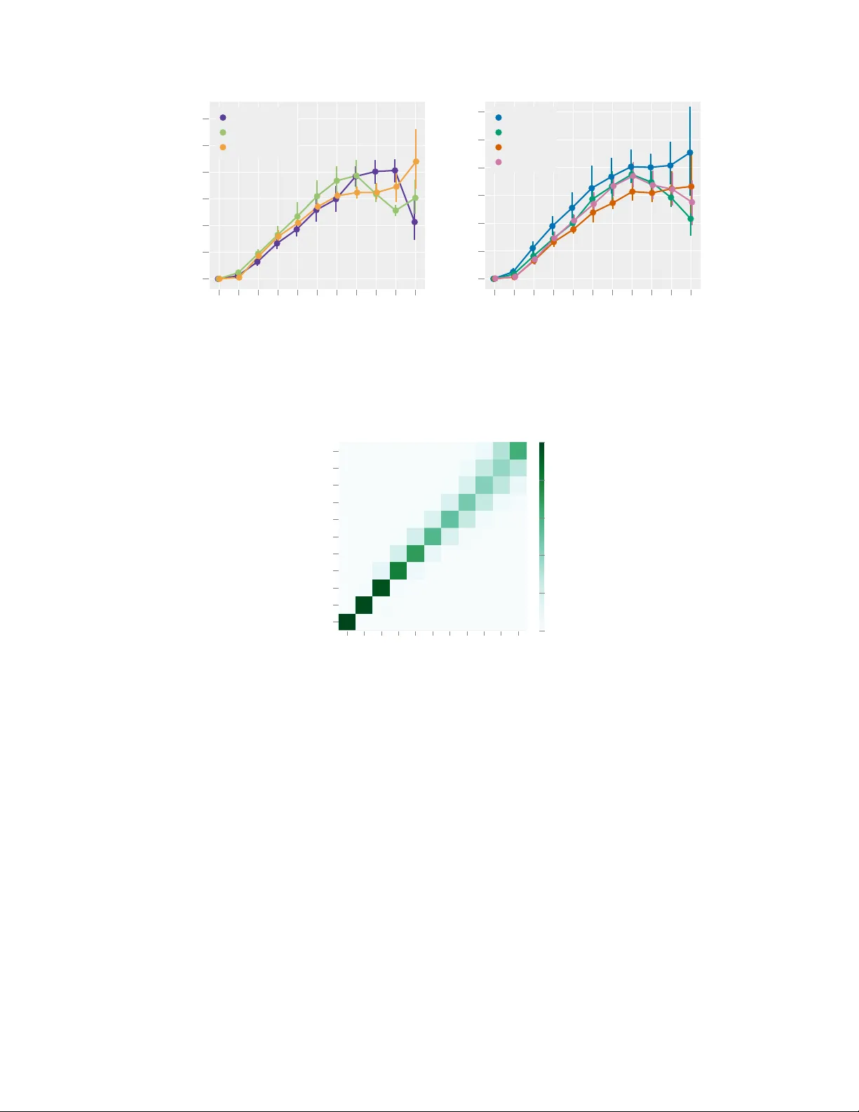
Classification vs. Regr ession in Supervised Lear ning f or Single Channel Speak er Count Estimation Fabian-Robert St ¨ oter International Audio Laboratories Erlangen ∗ fabian-robert.stoeter@audiolabs-erlangen.de Soumitro Chakrabarty International Audio Laboratories Erlangen soumitro.chakrabarty@audiolabs-erlangen.de Bernd Edler International Audio Laboratories Erlangen bernd.edler@audiolabs-erlangen.de Emanu ¨ el A. P . Habets International Audio Laboratories Erlangen emanuel.habets@audiolabs-erlangen.de Abstract The task of estimating the maximum number of concurrent speakers from single channel mixtures is important for various audio-based applications, such as blind source separation, speaker diarisation, audio surveillance or auditory scene clas- sification. Building upon po werful machine learning methodology , we develop a Deep Neural Network (DNN) that estimates a speaker count. While DNNs effi- ciently map input representations to output targets, it remains unclear ho w to best handle the network output to infer integer source count estimates, as a discrete count estimate can either be tackled as a regression or a classification problem. In this paper , we in v estigate this important design decision and also address comple- mentary parameter choices such as the input representation. W e e v aluate a state- of-the-art DNN audio model based on a Bi-directional Long Short-T erm Memory network architecture for speaker count estimations. Through experimental e v alu- ations aimed at identifying the best o verall strate gy for the task and sho w results for fiv e seconds speech segments in mixtures of up to ten speakers. 1 Introduction In a “cocktail-party” scenario with many concurrent speakers, different applications may be envi- sioned such as localization, cro wd monitoring, surv eillance, speech recognition or speaker separa- tion. In this scenario, a typical assumption is that the number of concurrent speakers is known, which turns out to be of paramount importance for the ef fectiveness of subsequent processings. Un- fortunately , in real world applications, information about the actual number of concurrent speakers is often not a v ailable. Surprisingly , v ery few methods hav e been proposed to address the task of counting the number of speakers. Estimating the maximum number of concurrent speakers is closely related to the more dif ficult problem of identifying them, which is the topic of speaker diarisation (who speaks when) [28]. W e call a system that identifies speakers first, “counting by detection”. These systems often use segments where only one speaker is acti ve to discriminate the speakers. Then comparisons of found ∗ International Audio Laboratories Erlangen is a joint institution of the Friedrich-Alexander-Uni versit ¨ at Erlangen-N ¨ urnberg (F A U) and Fraunhofer Institute for Integrated Circuits (IIS). A 0 . 0 0 . 6 1 . 2 1 . 9 2 . 5 3 . 0 T i m e i n s e c o n d s k = 3 2 2 2 3 3 3 3 B C Figure 1: Illustration of our application scenario of three concurrent speakers and their respecti ve speech activity . Bottom plot sho ws the number of concurrently acti ve speakers and its maximum k which is our targeted output. segments are made to discriminate and temporally locate the speakers within a giv en recording. When sources are fully overlapped as in real “cocktail party” en vironments, such a segmentation is hardly feasible. And when a speaker o verlap is as prev alent as in a “cocktail-party” scenario, dev eloping an algorithm to detect speakers is challenging. In this study we therefore attempt to directly estimate a speaker count instead of counting them after identification. W e refer to this strategy as “direct count estimation”. In multichannel signal processing, count estimation usually is achieved by estimating directions of arriv al (DoA) and clustering them [22, 30]. The first single channel method, based on thresholding amplitude modulation patterns, was proposed in [3]. In [25], the authors propose an energy feature based on temporally averaged mel-scale filter outputs. In a more recent work [32], the number of speakers is estimated by applying hierarchical clustering on fixed-length audio segments. The main weakness of this method is to rely on the assumption that there are segments where only one speaker is acti ve. In another vein, Andrei et.al. [2] proposed an algorithm which correlates single frames of multi-speaker mixtures with a set of single-speaker utterances. Motiv ated by the recent and impressiv e successes of deep learning approaches in various audio-related tasks [13, 33], we focus on dev eloping such a method for direct count estimation. In computer vision, (object) count estimation using DNNs has recently achie ved state-of-the-art performance [4, 5, 7, 17, 20, 27, 31, 34, 35]. T wo main paradigms may be found in the literature for this purpose, namely , re gr ession and classification . In this work we w ant to build upon these findings to achieve direct count estimation of speakers. Our main contributions are: i) to formulate the speaker count estimation problem as either a classifica- tion or a regression task, and ii) to propose a neural network architecture based on a state-of-the-art BLSTM network, to infer the number of speakers from short audio segments of 5s. Finally , we present experimental results for the dif ferent problem formulations as well as input feature repre- sentations to identify the best strategy for this task. For the sake of reproducibility , pre-trained network and the test dataset are made a vailable for do wnload on the accompanying website. 2 2 Problem F ormulation W e consider the task of estimating the maximum number of concurrent speakers, k ∈ Z + 0 , in a single channel audio mixture x . This is achiev ed by applying a mapping from x to k . Let x be a time domain signal of N samples, representing a linear mixture of L unique single speaker speech signals s l . Naturally , not all speakers l = 1 , . . . , L are acti ve at ev ery time instance. W e therefore, for each sample n , introduce a latent binary speech activity variable v nl ∈ { 0 , 1 } . Then, our task is to estimate k = max n L X l =1 v nl ! . (1) It can be seen that our proposed task of estimating k ≤ L is more closely related to source separation whereas the estimation of L itself is more useful for tasks where speakers do not ov erlap. W e 2 https://www.audiolabs- erlangen.de/resources/2017- CountNet ii assume that no additional prior information except the maximum number of concurrent speakers, k max , is available, representing an upper limit for estimation. In Figure 1, we illustrate our setup in a “cocktail-party” scenario featuring L = k = 3 speakers. For the DNN system proposed in this paper , we use a non-negati ve time-frequency (TF) input representation X ∈ R D × F + instead of x , where D and F denote the total number of time frames and frequency sub-bands, respecti vely . 2.1 Estimation in a Deep Learning Framework In this study , we choose a deep neural network (DNN) as the mapping function f θ from the input X to the output y , gi ven by y = f θ ( X ) , where the optimal parameters (weights) θ are learned via supervised training. The output of the DNN is not necessarily the direct source count k , therefore we introduce q ( · ) as a decision function , such that ˆ k = q ( f θ ( X )) . (2) The DNN is trained in a supervised manner using a training database of { X , k } examples. In this work, we w ant to in vestigate three dif ferent choices for the output distrib utions of the DNN, as well as the corresponding decision functions q ( · ) . Classification : Here the output distrib ution is directly taken as discrete , discarding any meaning concerning the ordering of the different possible values. Giv en some particular input X , the net- work generates the posterior output probability for ( k max + 1) classes (including k = 0 ) using the softmax activ ation function, and a maximum a posteriori (MAP) decision function is chosen that simply picks the most likely class q = arg max( · ) . Notwithstanding its conceptual simplicity , clas- sification has two drawbacks. First, the intuiti ve ranking between different estimates is lost: e.g. p ( k = 6) may not depend on p ( k = 5) . Second, the largest possible count k max is given a priori . Despite these limitations, classification-based approaches have successfully been applied in deep neural networks for counting objects [17, 27, 35] in images. Gaussian Regression : In regression, k is deri ved from an output distribution defined on the real line. The output distribution in this setting is assumed to be Gaussian and the associated cost func- tion is the classical squared error . During inference and given the output f θ ( X ) of the network, the best discrete value that is consistent with the model is simply the rounding operator q = [ · ] . Gaus- sian regression has achie ved state-of-the-art counting performance in computer vision using deep learning framew orks [4, 5, 20, 34]. Discrete Poisson modelling : When it comes to modelling count data, it is often shown effecti ve to adopt the Poisson distribution [9]. First, this strategy retains the advantage of the classification approach to directly pick a probabilistic model over the actual discrete observations, a voiding the somewhat artificial trick of introducing a latent v ariable that would be rounded to yield the observa- tion. Second, the model av oids the inconv enience of the classification approach to completely drop dependencies between classes. Due to these advantages, the Poisson distribution has been used in studies devising deep architectures for counting systems [24]. For instance in [6, 9, 24], it is shown that the number of objects in images can be well modelled by the Poisson distribution. Inspired by these pre vious works, we also consider the Poisson output distribution P ( k | f θ ( X )) where P ( · | λ ) denotes the Poisson distribution with scale parameter λ . In this setup, the cost function at learning time is the Poisson negativ e log-likelihood and the deep architecture at test time pro vides the predicted scale parameter f θ ( X ) ∈ R + , which summarizes the whole output distribution. As a decision function q in this setting, we considered several alternativ es. A first option is to again resort to MAP estimation and pick the mode [ f θ ( X )] of the distrib ution as a point estimate. Howe ver , experiments sho wed that the posterior median yields better estimates, and is given by q ( f θ ( X )) = argmin ˆ k ∞ X k =0    ˆ k − k    P ( k | f θ ( X )) (3a) = median ( k ∼ P ( f θ ( X ))) (3b) where the median of a Poisson distributed random variable was approximated giv en the expression in [8]. iii Output T ype Activ ation Dim. Loss Classification Softmax B k max +1 Cat. cross entropy Gaussian Regr . Linear R 1 MSE Poisson Regr . Exponential R 1 Neg. log likelihood T able 1: Output Activ ation Functions and Loss Functions 3 Proposed Model V arious audio-related applications share common DNN architecture designs, often found by incor- porating domain knowledge and through extensi ve hyperparameter searches. For our proposed task of source count estimation, howe ver , domain knowledge is dif ficult to incorporate, as this study aims at rev ealing the best strategy to address the problem. Therefore, we use a network built upon an ex- isting BLSTM-RNN architecture, that has already shown a considerable amount of generalization for various audio applications [12, 19]. A recurrent neural network (RNN) is very similar to a fully connected network, except that RNN applies the same set of weights recursiv ely ov er an input sequence. RNNs can detect structure in sequential data of arbitrary length. This makes it ideal to model time series, ho we ver , in practice, the temporal context learnt is limited to only a fe w time instances, because of the vanishing gradient problem [14]. T o alle viate this problem, forgetting factors (also called gating) were proposed. One of the most popular gated recurrent cells is the Long Short-T erm Memory (LSTM) [15] cell. Its effecti veness has been prov en in various applications and LSTMs are the state-of-the-art approach for speech recognition [11] or singing voice detection [19]. In this work we employed a bi-directional LSTM (BLSTM) with three hidden layers whose sizes are 30, 20 and 40 similar to the architecture intro- duced in [19]. A BLSTM is more robust compared to a simple LSTM, since input information from both past as well as the future in used to learn the weights. For further information on BLSTMs, the reader is referred to [10]. For a gi ven input sequence, the output of a recurrent layer is either only the last step output or a full sequence. W e found that employing the full sequence output of the last recurrent layer before feeding it into the fully connected output layer is important in the context of RNNs for count estimation. Furthermore we added a temporal max pooling layer with pooling size 2 to reduce the number of parameters for the fully connected layer . T emporal max pooling intuitiv ely fits to our problem formulation which in itself is a maximum of the number of sources in a specific number of frames. As we introduced in Section 2.1, the count estimation problem can be addressed using three dif ferent strategies. For each of the decision functions a suitable output activ ation and loss is used as shown in T able 1. Except for these (output) parameters, all models hav e the same parameters. 4 T raining Since a realistic dataset of fully ov erlapped speakers is not av ailable, we chose to generate syn- thetic mixtures. W e recognize that in a simulated “cocktail-party” en vironment, mixtures lack the con versational aspect of human communication but provide a controlled en vironment which helps understand how a DNN solves the count estimation problem. As we aim for a speaker independent solution, we selected a speech corpus with a large number of different speakers instead of lar ge number of utterances, yielding a larger number of unique mixtures. For training we selected the LibriSpeech clean-360 [23] dataset which includes 363 hours of clean speech of English utterances from 921 speakers (439 female and 482 male speakers). As rev ealed in Section 2, the maximum number of concurrent speakers k requires annotation of the activity of each indi vidual speaker . Even though LibriSpeech comes with annotations, they often are not consistent across dif ferent corpora. W e therefore generated annotations based on a v oice activity detection algorithm (V AD). In this work, we used the implementation from the Chromium W eb Br owser that is part of the W ebR TC Standard [1]. iv T o generate a single training sample { X , k } , we draw a unique set of L speakers from the corpus. For each of the speakers we then select a random utterance, resampled to 16 kHz sampling rate and apply V AD. The V AD method w as configured using a hop size of 10 ms. Further, the V AD estimate was used to remove silence in the beginning and the end of an utterance recording. In the next step, more utterances from the same speaker are drawn from the corpus until the desired duration is reached. Both, the audio recording and the V AD annotation of each utterance is concatenated. The procedure is repeated for all speakers so that L time domain signals are created. The signals are mixed and peak normalized to avoid clipping. Mixtures are then transformed to a time-frequency matrix X ∈ D × F as defined in Section 2. The ground truth output k are then computed using the V AD matrix based on Equation 1. W e follo w the proposal of [31] and include non-speech examples in our training data to a void using zero input samples for k = 0 . F or this, we used the TUT Acoustic Scenes dataset [21] to create negati ve training samples using the same procedure as described above. Because these en viron- mental sounds could include speech, scenes with cafe/restaurant , grocery store and metro station were omitted. As our application closely relates to source separation it is desirable for our trained DNN system to be robust against gain variations. W e therefore find it important to make sure that the DNN cannot lev erage the gain factors of the mixture. W e found that the av eraged energy of one bin across all frames of the input sample already is a solid indicator for the number of speakers. T o accomodate these findings, we normalize X to the a verage Euclidean norm of all frames as used in [29]. Additionally , as common in machine learning, we scale the normalized input representation so that the feature dimensions ha ve zero mean and unit v ariance/standard de viation across the whole training dataset. T o train the network we use Poisson sampling to balance the number of samples T k for each k . For our experiments we chose a medium-sized training dataset of T k = 1820 samples ∀ k ∈ [0 , . . . , 10] resulting in a total of 20,020 training items, each containing 10 seconds of audio, resulting in 55.55 hours of training material. The actual duration of each input is reduced to five seconds by selecting a random excerpt from each mixture. F or each excerpt Equation 1 is ev aluated to generate a single sample, then combined into mini-batches of 32 samples. This way the network is seeing slightly different samples (in dif ferent order) in each training epoch. W e found this procedure (also used in [26]) to help speeding up the stochastic gradient based training process. The DNN is trained using the AD AM optimizer [18]. In addition to the training dataset we created a separate validation dataset of T k = 5720 samples using a different set of speakers from LibriSpeech dev-clean . Early stopping is applied by monitoring the validation loss to reduce the effect of overfitting. Training nev er exceeded 50 epochs. 5 Evaluation W e e valuated our proposed network architecture with tw o main parameters: the three proposed out- put distributions (see Section 2) and four dif ferent input representations. T o allow for a controlled test environment and at the same time limit the number of training iterations, we fix certain param- eters: In our experiment all speakers were mixed to 0 dB SNR. For all experimental parameters we ran the training three times with dif ferent random seeds for each run and report a veraged the results to minimize random effects caused by early stopping. W e used the LibriSpeech test-clean subsets to generate 5720 unique and unseen speaker mixtures of five seconds duration for the test set with k max = L = 10 . Since we are dealing with a novel task description, related speaker count estimation techniques like those introduced in Section 1, could hardly be used as baselines. Specifically , [32] does not work on fully o verlapped speech, [2] does not scale to the size of our dataset, since it requires to cross- correlate the full database against another . Finally , [25] proposes a feature but does not employ a fully automated system. W e translated this method into a data-dri ven approach and employed a vec- tor quantizer to get an optimal mapping with respect to the sum of squares criterion (we refer to this as VQ ). v 0 1 2 3 4 5 6 7 8 9 10 0.0 0.2 0.4 0.6 0.8 1.0 1.2 k MAE Classification Gaussian Regr . Poisson Regr . (a) Output Distribution 0 1 2 3 4 5 6 7 8 9 10 0.0 0.2 0.4 0.6 0.8 1.0 1.2 k MAE MEL40 MFCC20 STFT STFTLOG (b) Feature Representation Figure 2: Mean absolute error (MAE) o ver ground truth count k = [0 . . . 10] . Error bars show the 95% confidence interv als. Results are averaged ov er the dif ferent feature representations (a) and output distributions (b). 0 1 2 3 4 5 6 7 8 9 10 0 1 2 3 4 5 6 7 8 9 10 k ˆ k 0.0 0.2 0.4 0.6 0.8 1.0 Figure 3: Normalized confusion matrix showing ˆ k ov er k for the test data of the best performing net- work (Output Distrib ution: Classification, Feature Representation: STFT). 5.1 Input Representations For our task, we chose sev eral dif ferent input representations, well-established in speech application. W e e xpect that a high frequency resolution is needed to discriminate time frequency bins with ov er- lapped speech se gments from those that only belong to a single speaker . W e compared the following input representations that were all based on a frame length of 25 ms: STFT : magnitude of the Short-time Fourier transform computed using Hann windows. The result- ing input is X ∈ R 500 × 201 . LOGSTFT : logarithmically scaled magnitudes from STFT representation using log(1 + S T F T ) . The resulting input is X ∈ R 500 × 201 . MEL40 : compute mapping from the STFT output directly onto Mel basis using 40 triangular filters. The resulting input is X ∈ R 500 × 40 . MFCC20 : First 20 Mel-frequency cepstral coefficients. The resulting input is X ∈ R 500 × 20 . vi Before feature transformation, all input files were resampled to 16 kHz sampling rate. All features are computed using a hop size of 10 ms. 5.2 Metric While the intermediate output y is treated as either a classification or a regression problem (See Section 2), we e valuate the final output k as a discrete regression problem. W e therefore e v aluate the performance using the mean absolute error (MAE), which is also used to ev aluate other count related tasks (c.f. [24, 34]). 5.3 Results T o find the best parameters, we performed training and e valuation for the parameters, resulting in 36 trained networks. On av erage each network was trained 33 epochs before early stopping was engaged. Training duration was about 800 seconds per epoch on a NVIDIA GTX 1080 GPU. W e present the results in terms of input representation and output distrib ution in Figure 2. One can see that the ov erall trend of the count error in MAE is similar regardless of the parametrisation: all models are able to reliably distinguish between k = 0 and k = 1 , follo wed by a nearly linear increase in MAE for k = [1 . . . 7] . For k > 7 it can be seen that the classification networks hav e learned the maximum of k across the dataset, hence the prediction error decreases when k reaches its maximum. This is because classification based models intrinsically ha ve access to the maximum number of sources determined by the output vector dimensionality . Figure 2a indicates that Classification outperforms the other two distrib utions while Poisson regres- sion performs better than Gaussian regression which confirms the findings made in [24] on object counts. With respect to the input representation, as shown in Figure 2b, despite its larger input di- mension, choosing linear STFT as generally results in a better performance compared to MEL40 , LOGSTFT or MFCC20 . A detailed analysis of all distrib ution and feature combinations, not shown here due to space con- straints, re veals that STFT + Classification performs best. This model achie ves results of (MAE 0 . 38 ± 0 . 28 ) for k = [0 . . . 10] while the VQ baseline (MAE 2 . 41 ± 1 . 08 ) only performs slightly bet- ter than a mean estimator predicting ˆ k = 5 (MAE 2 . 73 ± 1 . 63 ). T o show the le vel of o verestimation or underestimation, we depict all responses in a confusion matrix (see Figure 3). Unlike humans that generally tend to underestimate for the task of speaker count estimation [16], one can see that our proposed model slightly ov erestimates for smaller k . 6 Conclusion and Outlook W e introduced the task of estimating the maximum number of concurrent speakers in a simulated “cocktail-party” en vironment using a data-driv en approach. W e e valuated three dif ferent methods to output integer source count estimates in conjunction with defining cost function over which to optimize. Our experiments revealed a tradeoff between better overall performance but requiring the maximum number of speakers to be estimated as prior kno wledge (classification) and slightly worse performance when treated as a regression problem using Poisson distribution. Furthermore, we in vestigated and ev aluated suitable input representations. Our final proposed BLSTM based classification model achieves mean absolute error of less than 0.4 speakers for zero to ten speakers. W e think this first study on data-dri ven speaker count estimation opens the field to interesting and new research. Future work would be to ev aluate and optimize other network structures such as con volutional neural networks and in vestigate the strategy a machine learning source count model pursues to solve the problem. Acknowledgments The authors gratefully acknowledge the compute resources and support provided by the Erlangen Regional Computing Center (RRZE). vii References [1] W ebR TC V AD v2.0.10. https://github.com/wiseman/py- webrtcvad/tree/2.0.10 . [2] V . Andrei, H. Cucuand, A. Buzo, and C. Burileanu. Counting competing speakers in a time frame - human versus computer . In Pr oc. Interspeech Conf. , 2015. [3] T . Arai. Estimating number of speakers by the modulation characteristics of speech. In Pr oc. IEEE (ICASSP) , volume 2, pages II–197, 2003. [4] C. Arteta, V . Lempitsky , and A. Zisserman. Counting in the wild. In Eur opean Conference on Computer V ision , pages 483–498. Springer , 2016. [5] L. Boominathan, S. S. Kruthiv enti, and R. V . Babu. Crowdnet: A deep con volutional network for dense crowd counting. In Pr oc. ACM Intl. Confer ence on Multimedia (ACMMM) , pages 640–644. A CM, 2016. [6] A. B. Chan and N. V asconcelos. Bayesian poisson regression for crowd counting. In Pr oc. IEEE Intl. Confer ence on Computer V ision (ICCV) , pages 545–551. IEEE, 2009. [7] P . Chattopadhyay , R. V edantam, R. R. Selvaraju, D. Batra, and D. Parikh. Counting everyday objects in ev eryday scenes. In Proc. Intl. IEEE Conf. on Computer V ision and P attern Recognition (CVPR) , July 2017. [8] K. P . Choi. On the medians of gamma distributions and an equation of ramanujan. Proceedings of the American Mathematical Society , 121(1):245–251, 1994. [9] N. Fallah, H. Gu, K. Mohammad, S. A. Seyyedsalehi, K. Nourijelyani, and M. R. Eshraghian. Nonlin- ear poisson regression using neural networks: a simulation study . Neural Computing and Applications , 18(8):939, 2009. [10] I. Goodfellow , Y . Bengio, and A. Courville. Deep Learning . MIT Press, 2016. http://www. deeplearningbook.org . [11] A. Gra ves, A. r . Mohamed, and G. Hinton. Speech recognition with deep recurrent neural networks. In Pr oc. IEEE (ICASSP) , pages 6645–6649, May 2013. [12] G. Hagerer , V . Pandit, F . Eyben, and B. Schuller . Enhancing LSTM RNN-Based speech o verlap detection by artificially mixed data. In Proc. A udio Eng. Soc. Conference on Semantic A udio , Jun 2017. [13] J. Hershey , Z. Chen, J. Le Roux, and S. W atanabe. Deep clustering: Discriminative embeddings for segmentation and separation. In Proc. IEEE (ICASSP) , pages 31–35, Mar . 2016. [14] S. Hochreiter . The vanishing gradient problem during learning recurrent neural nets and problem solu- tions. Int. J . Uncertain. Fuzziness Knowl.-Based Syst. , 6(2):107–116, Apr . 1998. [15] S. Hochreiter and J. Schmidhuber . Long short-term memory . Neural Comput. , 9(8):1735–1780, Nov . 1997. [16] T . Kawashima and T . Sato. Perceptual limits in a simulated cocktail party . Attention, P er ception and Psychophysics , 77(6):2108–2120, 2015. [17] A. Khan, S. Gould, and M. Salzmann. Deep con volutional neural networks for human embryonic cell counting. In Eur opean Conference on Computer V ision , pages 339–348. Springer , 2016. [18] D. P . Kingma and J. Ba. Adam: A method for stochastic optimization. In ICLR , 2014. [19] S. Leglai ve, R. Hennequin, and R. Badeau. Singing voice detection with deep recurrent neural networks. In Pr oc. IEEE (ICASSP) , pages 121–125, April 2015. [20] M. Marsden, K. McGuiness, S. Little, and N. E. O’Connor . Fully con volutional crowd counting on highly congested scenes. arXiv pr eprint arXiv:1612.00220 , 2016. [21] A. Mesaros, T . Heittola, and T . V irtanen. TUT database for acoustic scene classification and sound ev ent detection. In Pr oc. European Signal Pr ocessing Conf. (EUSIPCO) , Budapest, Hungary , 2016. [22] S. Mirzaei, Y . Norouzi, et al. Blind audio source counting and separation of anechoic mixtures using the multichannel complex nmf frame work. Signal Processing , 115:27–37, 2015. [23] V . Panayoto v , G. Chen, D. Povey , and S. Khudanpur . Librispeech: an asr corpus based on public domain audio books. In Pr oc. IEEE (ICASSP) , pages 5206–5210. IEEE, 2015. [24] S. H. Rezatofighi, V . K. BG, A. Milan, E. Abbasnejad, A. Dick, and I. Reid. DeepSetNet: Predicting sets with deep neural networks. In Pr oc. IEEE Intl. Confer ence on Computer V ision (ICCV) , 2017. [25] H. Sayoud and S. Ouamour . Proposal of a new confidence parameter estimating the number of speakers-an experimental in vestigation. Journal of Information Hiding and Multimedia Signal Pr ocessing , 1(2):101– 109, 2010. [26] J. Schl ¨ uter . Learning to pinpoint singing voice from weakly labeled examples. In Pr oc. of ISMIR) , pages 44–50, 2016. viii [27] S. Segu ´ ı, O. Pujol, and J. V itria. Learning to count with deep object features. In Pr oc. Intl. IEEE Conf. on Computer V ision and P attern Recognition (CVPR) , pages 90–96, 2015. [28] S. E. T ranter and D. A. Reynolds. An ov erview of automatic speaker diarization systems. IEEE T rans. Audio, Speec h, Lang. Pr ocess. , 14(5):1557–1565, 2006. [29] S. Uhlich, F . Giron, and Y . Mitsufuji. Deep neural network based instrument extraction from music. In Pr oc. IEEE (ICASSP) , pages 2135–2139, April 2015. [30] O. W alter , L. Drude, and R. Haeb-Umbach. Source counting in speech mixtures by nonparametric bayesian estimation of an infinite Gaussian mixture model. In Pr oc. IEEE (ICASSP) , pages 459–463, 2015. [31] C. W ang, H. Zhang, L. Y ang, S. Liu, and X. Cao. Deep people counting in extremely dense crowds. In Pr oc. ACM Intl. Confer ence on Multimedia (ACMMM) , pages 1299–1302. A CM, 2015. [32] C. Xu, S. Li, G. Liu, Y . Zhang, E. Miluzzo, Y .-F . Chen, J. Li, and B. Firner . Crowd++: Unsupervised speaker count with smartphones. In Proceedings of the 2013 A CM UbiComb 13 , pages 43–52. A CM, 2013. [33] D. Y u, M. K olbæk, Z.-H. T an, and J. Jensen. Permutation in variant training of deep models for speaker- independent multi-talker speech separation. In Pr oc. IEEE (ICASSP) , 2017. [34] C. Zhang, H. Li, X. W ang, and X. Y ang. Cross-scene crowd counting via deep con volutional neural networks. In Pr oc. Intl. IEEE Conf. on Computer V ision and P attern Recognition (CVPR) , pages 833– 841, 2015. [35] J. Zhang, S. Ma, M. Sameki, S. Sclaroff, M. Betke, Z. Lin, X. Shen, B. Price, and R. Mech. Salient object subitizing. In Pr oc. of the IEEE Conf. on Computer V ision and P attern Recognition (CCVPR) , pages 4045–4054, 2015. ix