Controllable Attention for Structured Layered Video Decomposition

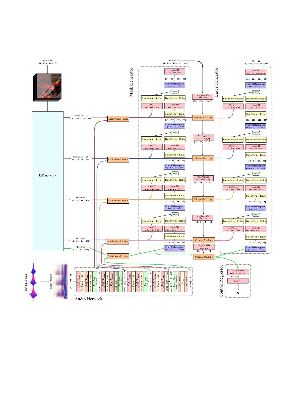
Contr ollable Attention f or Structur ed Layer ed V ideo Decomposition Jean-Baptiste Alayrac 1 ∗ Jo ˜ ao Carreira 1 ∗ Relja Arandjelovi ´ c 1 Andre w Zisserman 1,2 { jalayrac,joaoluis } @google.com 1 DeepMind 2 VGG, Dept. of Engineering Science, Uni v ersity of Oxford Abstract The objective of this paper is to be able to separate a video into its natural layers, and to contr ol which of the separated layer s to attend to. F or example , to be able to separate r eflections, transpar ency or object motion. W e make the following thr ee contributions: (i) we in- tr oduce a new structur ed neural network ar chitectur e that explicitly incorpor ates layers (as spatial masks) into its de- sign. This impr oves separation performance over pr evious general purpose networks for this task; (ii) we demonstrate that we can augment the ar chitectur e to leverag e external cues such as audio for contr ollability and to help disam- biguation; and (iii) we experimentally demonstrate the ef- fectiveness of our appr oach and training pr ocedure with contr olled experiments while also showing that the pro- posed model can be successfully applied to real-wor d ap- plications such as r eflection r emoval and action r ecognition in clutter ed scenes. 1. Introduction “The more you look the more you see”, is generally true for our complex, ambiguous visual world. Consider the ev- eryday task of cleaning teeth in front of a mirror . People performing this task may first attend to the mirror surf ace to identify any dirty spots, clean them up, then switch atten- tion to their mouth reflected in the mirror . Or they may hear steps behind them and switch attention to a new face now reflecting in the mirror . Not all visual possibilities can be in vestigated at once giv en a fix ed computational b udget and this creates the need for such controllable attention mecha- nisms. Layers offer a simple but useful model for handling this complexity of the visual w orld [ 51 ]. They provide a com- positional model of an image or video sequence, and cover a multitude of scenarios (reflections, shado ws, occlusions, haze, blur , ...) according to the composition rule. For exam- ple, an additiv e composition models reflections, and occlu- ∗ Equal contribution. Figure 1: W e propose a model, C 3 , able to decompose a video into meaningful layers. This decomposition process is controllable through external cues such as audio , that can select the layer to output. sion is modelled by superim posing opaque layers in a depth ordering. Giv en a a layered decomposition, attention can switch between the various layers as necessary for the task at hand. Our objective in this paper is to separate videos into their constituent layers, and to select the layers to attend to as illustrated in Figure 1 . A number of recent works hav e used deep learning to separate layers in images and videos [ 3 , 12 , 16 , 18 , 26 , 58 ], with varying success, but the selection of the layers has either had to be hard coded into the architecture, or the layers are arbitrarily mapped to the outputs. F or example, [ 3 ] considers the problem of sepa- rating blended videos into component videos, but because the mapping between input videos and outputs is arbitrary , training is forced to use a permutation in variant loss, and there is no control o ver the mapping at inference time. How can this symmetry between the composed input layers and output layers be broken? The solution explored here is based on the simple fact that videos do not consist of visual streams alone, they also hav e an audio stream; and, significantly , the visual and au- 1 dio streams are often correlated. The correlation can be strong (e.g. the synchronised sound and movement of beat- ing on a drum), or quite weak (e.g. street noise that separates an outdoor from indoor scene), b ut this correlation can be employed to break the symmetry . This symmetry breaking is related to recent approaches to the cocktail party audio separation problem [ 2 , 15 ] where visual cues are used to select speakers and improve the quality of the separation. Here we use audio cues to select the visual layers. Contributions: The contributions of this paper are three- fold: (i) we propose a ne w structured neural network archi- tecture that explicitly incorporates layers (as spatial masks) into its design; (ii) we demonstrate that we can augment the architecture to leverage external cues such as audio for controllability and to help disambiguation; and (iii) we e x- perimentally demonstrate the effecti veness of our approach and training procedure with controlled experiments while also showing that the proposed model can be successfully applied to real-word applications such as r eflection r emoval and action r ecognition in clutter ed scenes . W e show that the new architecture leads to improved layer separation. This is demonstrated both qualitativ ely and quantitati vely by comparing to recent general purpose models, such as the visual centrifuge [ 3 ]. For the quanti- tativ e e valuation we ev aluate how the downstream task of human action recognition is affected by reflection remov al. For this, we compare the performance of a standard action classification network on sequences with reflections, and with reflections removed using the layer architecture, and demonstrate a significant improv ement in the latter case. 2. Related work Attention contr ol. Attention in neural network modelling has had a significant impact in natural language processing, such as machine translation, [ 5 , 49 ] and vision [ 54 ], where it is implemented as a soft masking of features. In these set- tings attention is often not directly e valuated, but is just used as an aid to improve the end performance. In this paper we in vestigate models of attention in isolation, aiming for high consistency and controllability . By consistency we mean the ability to maintain the focus of attention on a particular target. By controllability we mean the ability to switch to a different tar get on command. V isual attentional control is actively studied in psychol- ogy and neuroscience [ 14 , 20 , 28 , 36 , 48 , 57 ] and, when malfunctioning, is a potentially important cause of condi- tions such as ADHD, autism or schizophrenia [ 33 ]. One of the problems studied in these fields is the relationship be- tween attention control based on top-down processes that are voluntary and goal-directed, and bottom-up processes that are stimulus-driv en (e.g. saliency) [ 27 , 48 ]. Another in- teresting aspect is the types of representations that are sub- ject to attention, often categorized into location-based [ 42 ], object-based or feature-based [ 6 ]: examples of the latter in- clude attending to anything that is red, or to anything that mov es. Another relev ant stream of research relates to the role of attention in multisensory integration [ 45 , 47 ]. Note also that attention does not always require eye movement – this is called covert (as opposed to overt ) attention. In this paper we consider cov ert attention as we will not be consid- ering active vision approaches, and focus on feature-based visual attention control. Cross-modal attention control. The idea of using one modality to control attention in the other has a long history , one notable application being informed audio source sepa- ration and denoising [ 7 , 21 , 39 , 52 ]. V isual information has been used to aid audio denoising [ 21 , 39 ], solve the cock- tail party problem of isolating sound coming from different speakers [ 2 , 15 , 37 , 52 ] or musical instruments [ 7 , 19 , 59 ]. Other sources of information used for audio source separa- tion include text to separate speech [ 32 ] and score to sepa- rate musical instruments [ 25 ]. More relev ant to this paper where audio is used for con- trol, [ 4 , 37 , 40 , 59 ] learn to attend to the object that is mak- ing the sound. Ho wever , unlike in this work, they do not directly output the disentangled video nor can they be used to remov e reflections as objects are assumed to be perfectly opaque. Other examples of control across modalities include tem- porally localizing a moment in a video using language [ 24 ], video summarization guided by titles [ 44 ] or query object labels [ 41 ], object localization from spoken words [ 23 ], image-text alignment [ 29 ], and interactive object segmen- tation via user clicks [ 9 ]. Layer ed video repr esentations. Layered image and video representations have a long history in computer vision [ 50 ] and are an appealing frame work for modelling 2.1D depth relationships [ 43 , 56 ], motion segmentation [ 50 ], reflec- tions [ 8 , 12 , 16 , 17 , 22 , 26 , 31 , 35 , 46 , 55 , 58 ], trans- parency [ 3 , 18 ], or ev en haze [ 18 ]. There is also evidence that the brain uses multi-layered visual representations for modelling transparency and occlusion [ 53 ]. 3. Appr oach This section describes the two technical contributions of this work. First, in Section 3.1 , a nov el architecture for decomposing videos into layers. This architecture is built upon the visual centrifuge [ 3 ], a generic U-Net like encoder- decoder , but extends it with two structural changes tailored tow ards the layered video decomposition task. Second, in Section 3.2 , the decomposition model is endo wed with con- trollability – the ability of the network to use external cues I3D Mask Generator Layer Generator Composition Module Encoder Decoder (a) Overview of the Compositional Centrifuge ( C 2 ) architectur e (b) Composition module Figure 2: Network architecture for layer decomposition ( 3.1 ). to control what it should focus on reconstructing. Here, we propose to use a natural video modality , namely audio , to select layers. Given this external cue, dif ferent mechanisms for controlling the outputs are in vestigated. Finally , in Sec- tion 3.3 , we describe how this model can be trained for suc- cessful controllable video decomposition. In the following, V stands for an input video. Formally , V ∈ R T × W × H × 3 where T is the number of frames, W and H are the width and height of the frames, and there are 3 standard RGB channels. The network produces an T × W × H × ( n × 3) tensor , interpreted as n output videos O , where each O i is of the same size as V . 3.1. Architectur e for lay er decomposition W e start from the visual centrifuge [ 3 ], a U-Net [ 38 ] encoder-decoder architecture, which separates an input video into n output videos. The encoder consists of an I3D network [ 11 ] and the decoder is composed by stacking 3D up con volutions. Howe ver , the U-Net architecture used there is generic and not tailored to the layered video decom- position task (this is verified experimentally in Section 4.1 ). Therefore, we propose two structural modifications specifi- cally designed to achie ve layered decomposition, forming a new network architecture, Compositional Centrifuge ( C 2 ) , shown in Figure 2a . Firstly , a bespoke gating mechanism is used in the encoder , which enables selection of scene seg- ments across space/time, thereby making the decoder’ s task easier . Secondly , layer compositionality is imposed by con- straining how the output videos are generated – the layer generator outputs multiple layers L and their composing coefficients β such that the output videos O are produced as a linear combination of the layers. These modifications are described in detail next. Encoder . W e aim to recover layers in the presence of occlu- sions and transparent surfaces. In such cases there are win- dows of opportunity when objects are fully visible and their appearance can be modelled, and periods when the objects are temporarily invisible or indistinguishable and hence can only be tracked. W e incorporate this intuition into a nov el spatio-temporal encoder architecture. The core idea is that the features produced by the I3D are gated with multiple ( m ) masks, also produced by the encoder itself. The gated features therefore already encode information about the un- derlying layers and this helps the decoder’ s task. In order to avoid gating all features with all m masks, which would be prohibiti vely expensi ve in terms of compu- tation and memory usage, feature channels are divided into m mutually-exclusi ve groups and each mask is applied only to the corresponding group. More formally , the mask generator produces M ∈ [0 , 1] T × W × H × m which is interpreted as a set of m spatio- temporal masks M = ( M c ) m c =1 . M is constrained to sum to 1 along the channel dimension by using a softmax non- linearity . Denote F l the output feature taken at lev el l in the I3D. W e assume that F l ∈ R T l × W l × H l × ( m × d l ) , i.e . the number of output channels of F l is a multiple of m . Giv en this, F l can be grouped into m features ( F c l ) m c =1 where F c l ∈ R T l × W l × H l × d l . The following transformation is ap- plied to each F c l : ˜ F c l = M c l  F c l , (1) where M c l is obtained by downsampling M c to the shape [ T l × W l × H l ] ,  refers to the Hadamard matrix product with a slight abuse of notation as the channel dimension is broadcast, i.e . the same mask is used across the channels. This process is illustrated in Figure 2a . Appendix B gives details on which feature lev els are used in practice. Imposing compositionality . In order to bias the decoder tow ards constructing layered decompositions, we split it into two parts – the layer generator produces m layers L and composing coefficients β which are then combined by the composition module to form the final n output videos O . The motiv ation is that individual layers should ideally represent independent scene units, such as moving objects, reflections or shadows, that can be composed in dif ferent ways into full scene videos. The proposed model architec- ture is designed to impose the inducti ve bias to wards this type of compositionality . More formally , the layer generator outputs a set of m layers L = ( L j ) m j =1 , where L j ∈ R T × H × W × 3 , and a set of n × m composing coef ficients β = ( β ij ) ( i,j ) ∈ [ [1 ,n ] ] × [ [1 ,m ] ] . These are then combined in the composition module (Fig- ure 2b ) to produce the final output videos O : O i = X j β ij  L j . (2) 3.2. Controllable symmetry br eaking The method presented in the previous section is inher- ently symmetric – the network is free to assign videos to output slots in any order . In this section, we present a strat- egy for controllable attention that is able to break the sym- metry by making use of side-information, a contr ol signal , provided as an additional input to the network. Audio is used as a natural control signal since it is readily av ailable with the video. In our mirror example from the introduction, hearing speech indicates the attention should be focused on the person in the mirror, not the mirror surface itself. For the rest of this section, audio is used as the contr ol signal , but the proposed approach remains agnostic to the control signal nature. Next, we explain ho w to compute audio features, fuse them with the visual features, and finally , how to obtain the output video which corresponds to the input audio. The ar- chitecture, named Contr ollable Compositional Centrifuge ( C 3 ) , is shown in Figure 3 . A udio network. The audio first needs to be processed be- fore feeding it as a control signal to the video decomposition model. W e follow the strategy employed in [ 4 ] to process the audio. Namely , the log spectrogram of the raw audio signal is computed and treated as an image, and a VGG-like network is used to extract the audio features. The network is trained from scratch jointly with the video decomposition model. A udio-visual fusion. T o feed the audio signal to the video model, we concatenate audio features to the outputs of the encoder before they get passed to the decoder . Since visual and audio features have dif ferent shapes – their sampling rates differ and they are 3-D and 4-D tensors for audio and vision, respecti vely – they cannot be concatenated nai vely . W e make the tw o features compatible by (1) a verage pool- ing the audio features o ver frequency dimension, (2) sam- pling audio features in time to match the number of tem- poral video feature samples, and (3) broadcasting the audio feature in the spatial dimensions. After these operations the audio tensor is concatenated with the visual tensor along the channel dimension. This fusion process is illustrated in Figure 3 . W e provide the full details of this architecture in Appendix B . Attention control. W e propose two strategies for obtain- ing the output video which corresponds to the input audio. log spectrogram Audio Network [T, W, H, C] Encoder Decoder Mean F . Pool [T',C'] T ime Sample [T,C'] [T,W,H, C'] Space broadcast Concat. [T', F, C'] Figure 3: The Controllable Compositional Centrifuge ( C 3 ) . The Encoder-Decoder components are the same as in C 2 (Fig- ure 2a ). Audio features are e xtracted from the audio control signal and fused with the visual features before entering the decoder . One is to use deterministic control where the desired video is forced to be output in a specific pre-defined output slot, without loss of generality O 1 is used. While simple, this strategy might be too rigid as it imposes too many con- straints onto the network. For example, a network might naturally learn to output guitars in slot 1 , drums in slot 2 , etc ., while deterministic control is forcing it to change this ordering at will. This intuition motiv ates our second strat- egy – internal pr ediction – where the network is free to produce output videos in any order it sees fit, b ut it also provides a pointer to the output slot which contains the de- sired video. Internal prediction is trained jointly with the rest of the network, full details of the architecture are giv en in Appendix B . The training procedure and losses for the two control strategies are described in the ne xt section. 3.3. T raining procedure T raining data. Since it is hard to obtain supervised training data for the video decomposition problem, we adopt and extend the approach of [ 3 ] and synthetically generate the training data. This by construction pro vides direct access to one meaningful ground truth decomposition. Specifically , we start from two real videos V 1 , V 2 ∈ R T × W × H × 3 . These videos are mixed together to generate a training video V ∈ R T × W × H × 3 : V = α  V 1 + ( 1 − α )  V 2 , (3) where α ∈ [0 , 1] T × W × H is a composing mask. W e explore two ways to generate the composing mask α . The first one is tr ansparent blending , used by [ 3 ], where α = 1 2 1 . While attractive because of its simplicity , it does not capture the full complexity of the real world composi- tions we wish to address, such as occlusions. For this rea- son, we also explore a second strategy , referred to as oc- clusion blending , where α is allo wed to v ary in space and takes values 0 or 1 . In more detail, we follow the proce- dure of [ 13 ] where spatio-temporal SLIC superpixels [ 1 ] are extracted from V 1 , and one is chosen at random. The compositing mask α is set to 1 inside the superpixel and 0 elsewhere; this produces mixtures of completely transparent or completely opaque spatio-temporal regions. The impact of the α sampling strategy on the final performance is ex- plored in Section 4.1 . T raining loss: without control. By construction, for an input training video V we know that one valid decompo- sition is into V 1 and V 2 . Howe ver , when training without contr ol , there is no easy way to know beforehand the order in which output videos are produced by the network. W e therefore optimize the network weights to minimize the fol- lowing permutation in variant reconstruction loss [ 3 ]: L pil ( { V 1 , V 2 } , O ) = min ( i,j ) | i 6 = j ` ( V 1 , O i ) + ` ( V 2 , O j ) , (4) where ` is a video reconstruction loss, e.g . a pix el wise error loss (see Section 4 for our particular choice). T raining loss: with control. When training with audio as the control signal, the audio of one video ( V 1 without loss of generality) is also provided. This potentially remov es the need for the permutation in variant loss required in the no- control case, b ut the loss depends on the choice of control strategy . The two proposed strategies are illustrated in Fig- ure 4 and described next. Deterministic contr ol loss. Here, the network is forced to output the desired video V 1 as O 1 so a natural loss is: L det ( { V 1 , V 2 } , O ) = ` ( V 1 , O 1 ) + ` ( V 2 , O 2 ) . (5) Note that for this loss the number of output videos has to be restricted to n = 2 . This limitation is another drawback of deterministic contr ol as it allo ws less freedom to propose multiple output video options. Internal pr ediction loss. In this strategy , the network freely decomposes the input video into outputs, and therefore the training loss is the same permutation in variant loss as for the no-control case ( 4 ). In addition, the network also points to the output which corresponds to the desired video, where the pointing mechanism is implemented as a module which outputs n real values s = ( s i ) n i =1 , one for each output video. These represent predicted dissimilarity between the Control Regressor Strategy 1: deter ministic c ontr ol Strategy 2: inter nal pr ed. contr ol Figure 4: A udio control strategies f or video decomposition. In this example, the inputs are the video V , a composition of V 1 showing a violin and V 2 showing drums, and an audio control sig- nal, A 1 , being the sound of the violin. W ith deterministic contr ol , V 1 is forced to be put in output slot O 1 (and therefore V 2 in O 2 ). W ith internal prediction contr ol , the netw ork can freely order the output videos, so is trained with the permutation inv ariant loss, but it contains an additional control regressor module which is trained to point to the desired output. desired video and output videos, and the attended output is chosen as arg min i s i . This module is trained with the fol- lowing re gression loss: L reg ( V 1 , s ) = n X i =1 | s i − ` ( V 1 , sg ( O i )) | , (6) where sg is the stop gradient operator . Stopping the gradient flow is important as it ensures that the only effect of training the module is to learn to point to the desired video. Its training is not allowed to influence the output videos themselves, as if it did, it could sacrifice the recon- struction quality in order to set an easier regression problem for itself. 4. Experiments This section e valuates the merits of the proposed Com- positional Centrifuge ( C 2 ) compared to pre vious work, per- forms ablation studies, in vestigates attention control via the audio control signal and the ef fectiv eness of the two pro- posed attention control strategies of the Controllable Com- positional Centrifuge ( C 3 ), follo wed by qualitativ e decom- position examples on natural videos, and ev aluation on the downstream task of action recognition. Model Loss (T ransp.) Loss (Occl.) Size Identity 0.364 0.362 – Centrifuge [ 3 ] 0.149 0.253 22.6M CentrifugePC [ 3 ] 0.135 0.264 45.4M C 2 w/o masking 0.131 0.200 23.4M C 2 0.120 0.190 27.1M T able 1: Model comparison in terms of a verage validation loss for synthetically generated videos with transp(arency) and occl(usions), as well as size in millions of parameters. All the results are obtained using models with n = 4 output layers. Cen- trifugePC is the predictor-corrector centrifuge [ 3 ], Identity is a baseline where the output videos are just copies of the input. Implementation details. Follo wing [ 3 , 34 ], in all experi- ments we use the following video reconstruction loss, de- fined for videos U and V as: ` ( U, V ) = 1 2 T X t k U t − V t k 1 + k∇ ( U t ) − ∇ ( V t ) k 1 ! , where k · k 1 is the L1 norm and ∇ ( · ) is the spatial gradient operator . All models are trained and e valuated on the blended v er- sions of the training and validation sets of the Kinetics-600 dataset [ 10 ]. T raining is done using stochastic gradient de- scent with momentum for 124k iterations, using batch size 128. W e employed a learning rate schedule, dividing by 10 the initial learning rate of 0.5 after 80k, 100k and 120k iter- ations. In all experiments we randomly sampled 64-frame clips at 128x128 resolution by taking random crops from videos whose smaller size being resized to 148 pixels. 4.1. Quantitative analysis In this section, we ev aluate the ef fectiv eness of our ap- proaches through quantitati ve comparisons on synthetically generated data using blended versions of the Kinetics-600 videos. Effectiveness of the C 2 architectur e f or video decomposi- tion. The baseline visual centrifuge achiev es a slightly bet- ter performance (lower loss) than originally reported [ 3 ] by training on clips which are twice as long (64 vs 32 frames). As can be seen in T able 1 , our proposed architecture outper- forms both the Centrifuge baseline [ 3 ], as well as the twice as large predictor-corrector model of [ 3 ]. Furthermore, both of our architectural improvements – the masking and the composition module – impro ve the performance (recall that the baseline Centrifuge is equiv alent to C 2 without the two improv ements). The improvements are especially apparent for occlusion blending since our architecture is explicitly designed to account for more complicated real-w orld blend- ing than the simple transpar ency blending used in [ 3 ]. T ransparent Occlusion Figure 5: Outputs of C 2 on blended Kinetics validation clips. Each ro w sho ws one example via a representativ e frame, with columns showing the input blended clip V , two output videos O 1 and O 2 , and the two ground truth clips V 1 and V 2 . T op three rows show the network is able to successfully decompose videos with transparencies. Bottom three rows show synthetic occlusions – this is a much harder task where, apart from having to detect the occlusions, the network also has to inpaint the occluded parts of each video. C 2 performs satisfactory in such a challenging sce- nario. Model Loss (T ransp.) Control Acc. C 2 0.120 50% (chance) C 3 w/ deterministic control 0.191 79.1% C 3 w/ internal prediction 0.119 77.7% T able 2: Model comparison on av erage validation reconstruction loss and control accuracy . The controllable models, C 3 , use audio as the control signal. Attention control. The effecti veness of the two proposed attention control strategies using the audio control signal is ev aluated next. Apart from comparing the reconstruc- tion quality , we also contrast the methods in terms of their contr ol accuracy , i.e . their ability to output the desired video into the correct output slot. For a giv en video V (composed of videos V 1 and V 2 ) and audio control signal A 1 , the output is deemed to be correctly controlled if the chosen output slot O c reconstructs the desired video V 1 well. Recall that the ‘chosen output slot’ is simply slot O c = O 1 for the deterministic contr ol , and predicted by the contr ol r egr essor as O arg min i ( s i ) for the internal pr e- T ransparent Occlusion Figure 6: V isualization of the internals of the compositional model. Recall that the C 2 model produces the output videos via the composition module (Figure 2b ) which multiplies the layers L with composing coefficients β . Here we visualize the individual β  L terms which when added together form the output videos. It can be observed that the layers and composing coefficient indeed decompose the input video V into its constituent parts, for both the transparent and occlusion blending. diction contr ol . The chosen output video O c is deemed to reconstruct the desired video well if its reconstruction loss is the smallest out of all outputs (up to a threshold t = 0 . 2 ∗ (max i ` ( V 1 , O i ) − min i ` ( V 1 , O i )) to account for potentially nearly identical outputs when outputing more than 2 layers): ` ( V 1 , O c ) < min i ` ( V 1 , O i ) + t . T able 2 ev aluates control performance across different models with the transpar ency blending . It sho ws that the non-controllable C 2 network, as expected, achiev es control accuracy equal to random chance, while the two control- lable variants of C 3 indeed exhibit highly controllable be- haviour . The two strategies are comparable on control ac- curacy , while internal pr ediction contr ol clearly beats deter - ministic contr ol in terms of reconstruction loss, confirming our intuition that deterministic control imposes o verly tight constraints on the network. 4.2. Qualitative analysis Here we perform qualitati ve analysis of the performance of our decomposition networks and inv estigate the internal layered representations. Figure 5 shows the video decompositions obtained from our C 2 network for transparent and occlusion blending. The network is able to almost perfectly decompose the videos with transparencies, while it does a reasonable job of re- constructing videos in the much harder case where strong occlusions are present and it needs to inpaint parts of the videos it has nev er seen. The internal representations produced by our layer gen- erator , which are combined in the composition module to produce the output videos, are visualized in Figure 6 . Our architecture indeed biases the model to wards learning com- positionality as the internal layers show a high degree of independence and specialize towards reconstructing one of the two constituent videos. Finally , Figure 7 sho ws qualitativ e results for the best controllable network, C 3 with internal prediction, where au- dio is used as the control signal. The network is able to ac- curately predict which output slot corresponds to the desired Figure 7: Qualitative results of C 3 with internal pr ediction. For visualization purposes, as it is hard to display sound, we show a frame of the video from which we use the audio as control on the left most column ( A 1 ). V (second column) represents the vi- sual input to the model. The right 4 columns are the outputs of C 3 . All examples exhibit good reconstruction error . The first four rows illustrate accurate control behaviour , where C 3 has correctly pre- dicted the output that corresponds to the contr ol signal (illustrated by a green marker under the frame). The last ro w illustrates an incorrect control (specified with a red marker under the wrongly chosen frame), where C 3 was fooled by a liquid sound that is plau- sible in the two scenarios. video, making fe w mistakes which are often reasonable due to the inherent noisiness and ambiguity in the sound. 4.3. Downstr eam tasks In the following, we inv estigate the usefulness of lay- ered video decomposition as a preprocessing step for other downstream tasks. Graphics. Layered video decomposition can be used in var - ious graphics applications, such as remov al of reflections, specularities, shadows, etc . Figure 8 shows some examples of decompositions of real videos. Compared with previous work of [ 3 ], as expected from the quantitative results, the decompositions are better as the produced output videos are more pure. Action recognition. A natural use case for video decom- position is action recognition in challenging scenarios with transparencies, reflections and occlusions. Since there are no action recognition datasets focused on such difficult set- tings, we again resort to using blended videos. A pre-trained I3D action recognition network [ 11 ] is used and its per- formance is measured when the input is pure unblended video, blended video, and decomposed videos, where the decomposition is performed using the best baseline model (predictor-corrector centrifuge, CentrifugePC [ 3 ]) or our Compositional Centrifuge ( C 2 ). For the pure video perfor - mance, we report the standard top-1 accuracy . For transpar ency blended videos, the desired outputs are both ground truth labels of the two constituent videos. Therefore, the models make two predictions and are scored 1, 0.5 and 0 depending on whether both predictions are cor - rect, only one or none is, respectiv ely . When I3D is applied directly on the blended video, the two predictions are natu- rally obtained as the tw o classes with the lar gest scores. For the decomposition models, each of the two output videos contributes their highest scoring prediction. In the case of occlusion blended videos, the desired out- put is the ground truth label of V 2 because there is not enough signal to reconstruct V 1 as the blended video only contains a single superpixel from V 1 . When I3D is applied directly on the blended video, the top prediction is used. The decomposition models tend to consistently reconstruct V 2 in one particular output slot, so we apply the I3D net- work onto the rele vant output and report the top-1 accurac y . T able 3 sho ws that decomposition significantly improv es the action recognition performance, while our C 2 strongly outperforms the baseline CentrifugePC [ 3 ] for both blend- ing strategies. There is still a gap between C 2 and the pure video performance, but this is understandable as blended videos are much more challenging. 5. Conclusion General vision systems, that can serve a v ariety of pur - poses, will probably require controllable attention mecha- nisms. There are just too man y possible visual narratives to in vestigate in natural scenes, for a system with finite com- putational power to pursue them all at once, always. In this paper we proposed a new compositional model for layered video representation and introduced techniques to make the resulting layers selectable via an external control signal – in Figure 8: Comparison of our C 2 model against [ 3 ] on r eal- world videos. The input video is sho wn on the left, and the output videos of C 2 and [ 3 ] are interleaved in the remaining columns for easier comparison. While both models manage to decompose the videos reasonably well, C 2 achiev es less leakage of one video into another . For e xample, C 2 versus [ 3 ] output O 1 (first ro w) removes the reflections of branches on the right side better , (second ro w) has fewer yellow circles of light, and (third row) makes the large circular reflection in the top half of the image much fainter . Mode Acc. (T ransp.) Acc. (Occl.) I3D – pure video 59.5 59.5 I3D 22.1 21.3 CentrifugePC [ 3 ] + I3D 34.4 21.5 C 2 + I3D 40.1 24.7 T able 3: Action recognition accuracy on the Kinetics-600 vali- dation set when the input to a pre-trained I3D classifier is a pure – non-blended – video (top row), a blended video directly passed through I3D, or a blended video that is first unblended using a layer decomposition model. The two columns sho w accuracies for two dif ferent blending processes: transparent and occluding. this case sound. W e showed that the proposed model can better endure automatically generated transparency and es- pecially occlusions, compared to pre vious work, and that the layers are selected based on sound cues with accuracies of up to 80% on the blended Kinetics dataset. As future work we would like to train our model on more naturally- looking occlusions, possibly by generating the composing mask using supervised segmentations instead of unsuper- vised superpixels. References [1] Radhakrishna Achanta, Appu Shaji, K evin Smith, Aurelien Lucchi, Pascal Fua, and Sabine S ¨ usstrunk. SLIC superpix- els compared to state-of-the-art superpixel methods. TP AMI , 2012. [2] T riantafyllos Afouras, Joon Son Chung, and Andrew Zis- serman. The Con versation: Deep Audio-V isual Speech En- hancement. In Interspeech , 2018. [3] Jean-Baptiste Alayrac, Jo ˜ ao Carreira, and Andrew Zisser- man. The visual centrifuge: Model-free layered video repre- sentations. In CVPR , 2019. [4] Relja Arandjelovi ´ c and Andrew Zisserman. Objects that sound. In ECCV , 2018. [5] Dzmitry Bahdanau, Kyunghyun Cho, and Y oshua Bengio. Neural machine translation by jointly learning to align and translate. arXiv pr eprint arXiv:1409.0473 , 2014. [6] Daniel Baldauf and Robert Desimone. Neural mechanisms of object-based attention. Science , 2014. [7] Zohar Barzelay and Y oav Y . Schechner . Harmony in motion. In CVPR , 2007. [8] Efrat Be’ery and Arie Y eredor . Blind Separation of Super- imposed Shifted Images Using Parameterized Joint Diago- nalization. T ransactions on Imag e Processing , 2008. [9] Y uri Y . Boyk ov and Marie-Pierre Jolly . Interacti ve graph cuts for optimal boundary & region segmentation of objects in N-D images. In ICCV , 2001. [10] Joao Carreira, Eric Noland, Andras Banki-Horv ath, Chloe Hillier , and Andrew Zisserman. A short note about kinetics- 600. In arXiv pr eprint arXiv:1808.01340 , 2018. [11] Joao Carreira and Andrew Zisserman. Quo vadis, action recognition? a new model and the kinetics dataset. In CVPR , 2017. [12] Zhixiang Chi, Xiaolin W u, Xiao Shu, and Jinjin Gu. Sin- gle Image Reflection Remov al Using Deep Encoder-Decoder Network. In arXiv pr eprint arXiv:1802.00094 , 2018. [13] Carl Doersch and Andrew Zisserman. Sim2real transfer learning for 3D pose estimation: motion to the rescue. In arXiv pr eprint arXiv:1907.02499 , 2019. [14] How ard E. Egeth and Steven Y antis. V isual attention: Con- trol, representation, and time course. Annual re view of psy- chology , 1997. [15] Ariel Ephrat, Inbar Mosseri, Oran Lang, T ali Dekel, Ke vin W ilson, A vinatan Hassidim, William T . Freeman, and Michael Rubinstein. Looking to Listen at the Cocktail Party: A Speaker-Independent Audio-V isual Model for Speech Separation. In SIGGRAPH , 2018. [16] Qingnan Fan, Jiaolong Y ang, Gang Hua, Baoquan Chen, and David W ipf. A Generic Deep Architecture for Single Image Reflection Remov al and Image Smoothing. In ICCV , 2017. [17] Hany Farid and Edward H. Adelson. Separating reflections and lighting using independent components analysis. In CVPR , 1999. [18] Y ossi Gandelsman, Assaf Shocher , and Michal Irani. “Double-DIP”: Unsupervised image decomposition via cou- pled deep-image-priors. In CVPR , 2019. [19] Ruohan Gao, Rogeris Feris, and Kristen Grauman. Learning to separate object sounds by watching unlabeled video. In CVPR , 2018. [20] Michael Gazzaniga and Richard B Ivry . Cognitive Neur o- science: The Biology of the Mind: F ourth International Stu- dent Edition . WW Norton, 2013. [21] Laurent Girin, Jean-Luc Schwartz, and Gang Feng. Audio- visual enhancement of speech in noise. The J ournal of the Acoustical Society of America , 2001. [22] Xiaojie Guo, Xiaochun Cao, and Y i Ma. Robust Separation of Reflection from Multiple Images. In CVPR , 2014. [23] David Harwath, Adri ` a Recasens, D ´ ıdac Sur ´ ıs, Galen Chuang, Antonio T orralba, and James Glass. Jointly dis- cov ering visual objects and spoken words from raw sensory input. In ECCV , 2018. [24] Lisa Anne Hendricks, Oliver W ang, Eli Shechtman, Josef Sivic, T rev or Darrell, and Bryan Russell. Localizing mo- ments in video with natural language. In ICCV , 2017. [25] Romain Hennequin, Bertrand David, and Roland Badeau. Score informed audio source separation using a parametric model of non-negati ve spectrogram. In ICASSP , 2011. [26] Daniel Heydeck er , Georg Maierhofer , Angelica I. A viles- Riv ero, Qingnan Fan, Carola-Bibiane Sch ¨ onlieb, and Sabine S ¨ usstrunk. Mirror , mirror , on the wall, who’ s got the clearest image of them all? – A tailored approach to single image reflection remov al. arXiv preprint arXiv:1805.11589 , 2018. [27] Laurent Itti, Christof K och, and Ernst Niebur . A model of saliency-based visual attention for rapid scene analysis. P AMI , 1998. [28] Laurent Itti, Geraint Rees, and John Tsotsos. Neur obiology of attention . Academic Press, 2005. [29] Andrej Karpathy and Li Fei-Fei. Deep visual-semantic align- ments for generating image descriptions. In CVPR , 2015. [30] Bruno K orbar , Du T ran, and Lorenzo T orresani. Coopera- tiv e learning of audio and video models from self-supervised synchronization. In NeurIPS , 2018. [31] Kun Gai, Zhenwei Shi, and Changshui Zhang. Blind Sepa- ration of Superimposed Moving Images Using Image Statis- tics. P AMI , 2012. [32] Luc Le Magoarou, Ale xe y Ozerov , and Ngoc Q.K. Duong. T ext-informed audio source separation. Example-based ap- proach using non-neg ativ e matrix partial co-factorization. Journal of Signal Pr ocessing Systems , 2015. [33] Eric Mash and David W olfe. Abnormal child psychology . Cengage Learning, 2012. [34] Michael Mathieu, Camille Couprie, and Y ann LeCun. Deep multi-scale video prediction beyond mean square error. In ICLR , 2016. [35] Ajay Nandoriya, Mohamed Elgharib, Changil Kim, Mo- hamed Hefeeda, and W ojciech Matusik. V ideo Reflection Remov al Through Spatio-T emporal Optimization. In ICCV , 2017. [36] Aude Oliv a, Antonio T orralba, Monica S Castelhano, and John M Henderson. T op-down control of visual attention in object detection. In ICIP , volume 1, pages I–253. IEEE, 2003. [37] Andrew Owens and Alexei A. Efros. Audio-visual scene analysis with self-supervised multisensory features. In ECCV , 2018. [38] Olaf Ronneberger , Philipp Fischer , and Thomas Brox. U- Net: Conv olutional Networks for Biomedical Image Seg- mentation. In MICCAI , 2015. [39] Dana Sege v , Y oav Y . Schechner, and Michael Elad. Example-based cross-modal denoising. In CVPR , 2012. [40] Arda Senocak, T ae-Hyun Oh, Junsik Kim, Ming-Hsuan Y ang, and In So Kweon. Learning to localize sound source in visual scenes. In CVPR , 2018. [41] Aidean Sharghi, Boqing Gong, and Mubarak Shah. Query- focused extracti ve video summarization. In ECCV , 2016. [42] Markus Siegel, T obias H Donner, Robert Oosten veld, Pas- cal Fries, and Andreas K Engel. Neuronal synchronization along the dorsal visual pathway reflects the focus of spatial attention. Neur on , 2008. [43] Paul Smith, T om Drummond, and Roberto Cipolla. Layered motion segmentation and depth ordering by tracking edges. P AMI , 26(4):479–494, 2004. [44] Y ale Song, Jordi V allmitjana, Amanda Stent, and Alejandro Jaimes. TVSum: Summarizing web videos using titles. In CVPR , 2015. [45] Charles Spence and Jon Dri ver . Audiovisual links in endoge- nous cov ert spatial attention. Journal of Experimental Psy- chology: Human P er ception and P erformance , 22(4):1005, 1996. [46] Richard Szeliski, Shai A vidan, and P . Anandan. Layer extraction from multiple images containing reflections and transparency . In CVPR , 2000. [47] Durk T alsma, Daniel Senkowski, Salvador Soto-Faraco, and Marty G W oldorff. The multifaceted interplay between at- tention and multisensory integration. T rends in cognitive sci- ences , 2010. [48] John Tsotsos, Scan M. Culhane, Wink y Y an Kei W ai, Y uzhong Lai, Neal Da vis, and Fernando Nuflo. Modeling visual attention via selectiv e tuning. Artificial Intelligence , 1995. [49] Ashish V aswani, Noam Shazeer , Niki Parmar , Jakob Uszko- reit, Llion Jones, Aidan N Gomez, Łukasz Kaiser, and Illia Polosukhin. Attention is all you need. In NIPS , 2017. [50] John Y A W ang and Edward H Adelson. Representing mov- ing images with layers. IEEE T ransactions on Image Pro- cessing , 3(5):625–638, 1994. [51] John Y . A. W ang and Edward H. Adelson. Representing moving images with layers. T ransactions on image pr ocess- ing , 1994. [52] W enwu W ang, Darren Cosker , Y ulia Hicks, Saeid Sanei, and Jonathon. Chambers. V ideo assisted speech source separa- tion. In ICASSP , 2005. [53] Michael A W ebster . Color vision: Appearance is a many- layered thing. Curr ent Biology , 2009. [54] Kelvin Xu, Jimmy Ba, Ryan Kiros, Kyunghyun Cho, Aaron Courville, Ruslan Salakhudinov , Rich Zemel, and Y oshua Bengio. Show , attend and tell: Neural image caption gen- eration with visual attention. In ICML , pages 2048–2057, 2015. [55] T ianfan Xue, Michael Rubinstein, Ce Liu, and W illiam T . Freeman. A Computational Approach for Obstruction-Free Photography. In SIGGRAPH , 2015. [56] Y i Y ang, Sam Hallman, Dev a Ramanan, and Charless Fo wlkes. Layered object detection for multi-class segmenta- tion. In CVPR , 2010. [57] Stev en Y antis. Control of visual attention. Attention , 1998. [58] Xuaner Zhang, Ren Ng, and Qifeng Chen. Single image reflection separation with perceptual losses. CVPR , pages 4786–4794, 2018. [59] Hang Zhao, Can Gan, Andrew Rouditchenko, Carl V ondrick, Josh McDermott, and Antonio T orralba. The sound of pixels. In ECCV , 2018. Overview In this appendix, we cov er three additional aspects: (i) in Section A we include an additional qualitati ve comparison on real videos, for which there w as not space in the original manuscript; (ii) Section B provides details for the network architecture; and finally (iii) in Section C we study how the network uses the audio for control, by perturbing the audio. A. Additional comparison of C 2 with pre vious work W e compare to previous work [ 3 , 55 ] on the task of re- flection remov al in Figure 9 . One of the baselines [ 55 ] uses geometrical modelling and optimization b ut under strict as- sumptions (e.g. rigid motion). The second baseline [ 3 ] is trained on the same data as our model. The proposed model generates a sharp video with little reflection left. B. Architecture details Figure 11 illustrates the architecture employed for C 2 while Figure 12 pro vides full details about the architecture employed for C 3 with internal pr ediction control strategy . C. Additional quantitative study f or C 3 What aspect of the audio control signal is used for the controlled decomposition? One hypothesis is that the net- work latches onto low-le vel synchronization cues, so that the desired output video is identified as the one that is in sync with the audio. An alternativ e is that the desired video is the one whose semantic content matches the audio. T o answer this question, we use the best trained C 3 net- work with internal prediction control and ev aluate its perfor- mance with respect to varying degrees of audio offset. The experiment is performed on the v alidation set of Kinetics- 600. Reconstruction loss remains completely unaf fected by shifting audio, while control accuracy deteriorates slightly as the of fset is increased, as shown in Figure 10 . The re- sults suggest that the network predominantly uses the se- mantic information contained in the audio signal as control accuracy only decreases by 1.4 percentage points with the largest of fsets where the audio does not ov erlap with the vi- sual stream. Howe ver , some synchronization information is probably used as audio offset does hav e an adverse ef fect on control accurac y , and there is a sharp drop at relati vely small offsets of 0.5-1s. There is scope for exploiting the synchronization signal further as it might provide a boost in control accuracy . A potential approach includes using a training curriculum analogous to [ 30 ]. Figure 9: Qualitati ve comparison of C 2 with other works. 0.0 0.5 1.0 1.5 2.0 2.5 3.0 Audio offset (s) 75.4 75.6 75.8 76.0 76.2 76.4 76.6 76.8 77.0 Control accurcy (%) Figure 10: Effect of shifting the control audio signal on the control accurac y . Note that the network w as trained and tested on 2.56 second clips, so a 2.56 second of fset corre- sponds to no ov erlap between the audio and visual streams. Conv3DT ranspose Conv3D Conv3D s=2, k= [2,4,4], C=64 [16, 1 4, 14, 6 4] BatchNorm + ReLu s=1, k= 1, C=64 s=1, k=[ 2,4,4], C=64 BatchNorm + ReLu BatchNorm + ReLu Concat. Conv3DT ranspose Conv3D Conv3D s=2, k= 4, C=64 [32, 2 8, 28, 6 4] BatchNorm + ReLu s=1, k= 1, C=64 s=1, k=4 , C=64 BatchNorm + ReLu BatchNorm + ReLu Concat. Conv3DT ranspose Conv3D Conv3D s=[1,2, 2], k=4, C=32 [32, 5 6, 56, 3 2] BatchNorm + ReLu s=1, k= 1, C=32 s=1, k=4 , C=32 BatchNorm + ReLu BatchNorm + ReLu Concat. Conv3DT ranspose Conv3D Conv3D s=[1,2, 2], k=4, C=32 [32, 1 12, 112, 32] BatchNorm + ReLu s=1, k= 1, C=16 s=1, k=4 , C=16 BatchNorm + ReLu BatchNorm + ReLu Concat. Conv3DT ranspose Conv3D s=2, k= 4, C=32 [64, 2 24, 224, 32] s=1, k= 4, C=m I3D network Mask Generator [32, 11 2, 112, 64] Conv3d_1a_7x7 [32, 56 , 56, 19 2] Conv3d_2c_3x3 [32, 28 , 28, 48 0] Mixed_3c [16, 14 , 14, 83 2] Mixed_4f [8, 7, 7, 1024] Mixed_5c [64, 22 4, 224, m + m*n ] Output Masks [64, 22 4, 224, 3] Input video A vgPool3D k=3, s= 2 [32, 11 2, 112, m] Channel Masking A vgPool3D [32, 56 , 56, m] k=3, s= [1,2,2] A vgPool3D [32, 28 , 28, m] k=3, s= [1,2,2] Channel Masking A vgPool3D [16, 14 , 14, m] k=3, s= 2 A vgPool3D [8, 7, 7, m] k=3, s= 2 Channel Masking Channel Masking Conv3DT ranspose Conv3D Conv3D s=2, k= [2,4,4], C=64 [16, 1 4, 14, 6 4] BatchNorm + ReLu s=1, k= 1, C=64 s=1, k=[ 2,4,4], C=64 BatchNorm + ReLu BatchNorm + ReLu Concat. Conv3DT ranspose Conv3D Conv3D s=2, k= 4, C=64 [32, 2 8, 28, 6 4] BatchNorm + ReLu s=1, k= 1, C=64 s=1, k=4 , C=64 BatchNorm + ReLu BatchNorm + ReLu Concat. Conv3DT ranspose Conv3D Conv3D s=[1,2, 2], k=4, C=32 [32, 5 6, 56, 3 2] BatchNorm + ReLu s=1, k= 1, C=32 s=1, k=4 , C=32 BatchNorm + ReLu BatchNorm + ReLu Concat. Conv3DT ranspose Conv3D Conv3D s=[1,2, 2], k=4, C=32 [32, 1 12, 112, 32] BatchNorm + ReLu s=1, k= 1, C=16 s=1, k=4 , C=16 BatchNorm + ReLu BatchNorm + ReLu Concat. Conv3DT ranspose Conv3D s=2, k= 4, C=32 [64, 2 24, 224, 32] s=1, k= 4, C=m*n +3*m Layer Generator Channel Masking [64, 22 4, 224, m*n+3*m ] Figure 11: Details of the architecture used for C 2 . The ‘Channel Masking‘ block corresponds to the masking procedure described in equation (1) of the main paper . Input 48kHz audio log spectrogram Conv3DT ranspose Conv3D Conv3D s=2, k= [2,4,4], C=64 [16, 1 4, 14, 6 4] BatchNorm + ReLu s=1, k= 1, C=64 s=1, k=[ 2,4,4], C=64 BatchNorm + ReLu BatchNorm + ReLu Concat. Conv3DT ranspose Conv3D Conv3D s=2, k= 4, C=64 [32, 2 8, 28, 6 4] BatchNorm + ReLu s=1, k= 1, C=64 s=1, k=4 , C=64 BatchNorm + ReLu BatchNorm + ReLu Concat. Conv3DT ranspose Conv3D Conv3D s=[1,2, 2], k=4, C=32 [32, 5 6, 56, 3 2] BatchNorm + ReLu s=1, k= 1, C=32 s=1, k=4 , C=32 BatchNorm + ReLu BatchNorm + ReLu Concat. Conv3DT ranspose Conv3D Conv3D s=[1,2, 2], k=4, C=32 [32, 1 12, 112, 32] BatchNorm + ReLu s=1, k= 1, C=16 s=1, k=4 , C=16 BatchNorm + ReLu BatchNorm + ReLu Concat. Conv3DT ranspose Conv3D s=2, k= 4, C=32 [64, 2 24, 224, 32] s=1, k= 4, C=m I3D network Mask Generator [32, 11 2, 112, 64] Conv3d_1a_7x7 [32, 56 , 56, 19 2] Conv3d_2c_3x3 [32, 28 , 28, 48 0] Mixed_3c [16, 14 , 14, 83 2] Mixed_4f [8, 7, 7, 1024] Mixed_5c [64, 22 4, 224, m + m*n ] Output Masks [64, 22 4, 224, 3] Input video A vgPool3D k=3, s= 2 [32, 11 2, 112, m] Channel Masking A vgPool3D [32, 56 , 56, m] k=3, s= [1,2,2] A vgPool3D [32, 28 , 28, m] k=3, s= [1,2,2] Channel Masking A vgPool3D [16, 14 , 14, m] k=3, s= 2 A vgPool3D [8, 7, 7, m] k=3, s= 2 Channel Masking Channel Masking Conv3DT ranspose Conv3D Conv3D s=2, k= [2,4,4], C=64 [16, 1 4, 14, 6 4] BatchNorm + ReLu s=1, k= 1, C=64 s=1, k=[ 2,4,4], C=64 BatchNorm + ReLu BatchNorm + ReLu Concat. Conv3DT ranspose Conv3D Conv3D s=2, k= 4, C=64 [32, 2 8, 28, 6 4] BatchNorm + ReLu s=1, k= 1, C=64 s=1, k=4 , C=64 BatchNorm + ReLu BatchNorm + ReLu Concat. Conv3DT ranspose Conv3D Conv3D s=[1,2, 2], k=4, C=32 [32, 5 6, 56, 3 2] BatchNorm + ReLu s=1, k= 1, C=32 s=1, k=4 , C=32 BatchNorm + ReLu BatchNorm + ReLu Concat. Conv3DT ranspose Conv3D Conv3D s=[1,2, 2], k=4, C=32 [32, 1 12, 112, 32] BatchNorm + ReLu s=1, k= 1, C=16 s=1, k=4 , C=16 BatchNorm + ReLu BatchNorm + ReLu Concat. Conv3DT ranspose Conv3D s=2, k= 4, C=32 [64, 2 24, 224, 32] s=1, k= 4, C=m*n +3*m Layer Generator Channel Masking [64, 22 4, 224, m*n+3*m ] Audio/V isual Fusion Audio/V isual Fusion Audio/V isual Fusion Audio/V isual Fusion Audio Network Conv2D s=2, k= 3, C=64 BatchNorm + ReLu [512, 2 56, 1] BatchNorm + ReLu conv1:[ 64, 32, 64] Conv2D s=2, k= 3, C=64 MaxPool s=2, k= 2 Conv2D s=1, k= 3, C=128 BatchNorm + ReLu BatchNorm + ReLu conv2:[ 32, 16, 128] Conv2D s=1, k= 3, C=128 MaxPool s=2, k= 2 Conv2D s=1, k= 3, C=256 BatchNorm + ReLu BatchNorm + ReLu conv3:[ 16, 8, 2 56] Conv2D s=1, k= 3, C=256 MaxPool s=2, k= 2 ReduceMax Time, F requency Conv2D s=1, k= 3, C=512 BatchNorm + ReLu BatchNorm + ReLu conv4:[ 16, 8, 5 12] Conv2D s=1, k= 3, C=512 ReLu FC: C=128 FC: C=128 fc2:[12 8] Control Regressor Audio/V isual Fusion FC: C=n A vgPool3D k=[8, 7 , 7], s= 1 [1152] Figure 12: Details of the architecture used for C 3 with internal prediction control. The ‘Channel Masking‘ block corresponds to the masking procedure described in equation (1) of the main paper . The ‘ Audio/V isual Fusion‘ block matches the A udio- visual fusion procedure described in Section 3.2 of the main paper and illustrated in Figure 3.