Rk-means: Fast Clustering for Relational Data

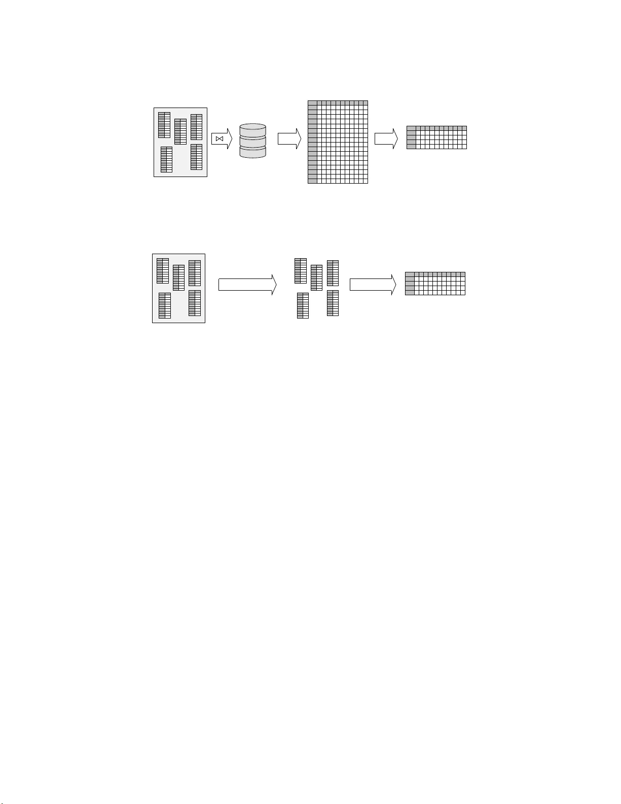
RK-MEANS: F AST CLUSTERING F OR RE LA TIONAL D A T A R Y AN CUR TIN, BEN MOSELEY, HUNG Q. NGO, XUANLON G NGUYEN, DAN OL TEANU, AND MAXIMILIAN SCHLEICH Abstract. Co n v en tional mac hine learning algorithms c annot be applied unt il a data matr ix is a v ailable to process. When the data matrix needs to b e obtained from a relational database via a feature extra ction query , t he computation cost can be prohibitive, as the data matrix may be (m uc h) l arger than the total input relation si ze. This pap er introduces Rk-means, or relational k -means algorithm, for clustering relational data tuples wi thout having to access the full data matrix. As such, w e av oid ha ving to run the expensive f eature extrac tion query and storing its output. Our algorithm lever ages the underlying s truct ures i n relational data. It inv olves construction of a s mall grid c or eset of the data matrix for subsequen t cluster construct ion. This giv es a constan t appro ximation for the k - means ob jective, while having asymptotic runt ime improv ements o v er standard approach es of first running the databa se query and then clustering. Empirical results show orders-of-magnitude sp eedup, and Rk-means can run faster on the database than even just computing the data matrix. 1. Introduction Clustering is an ubiquit ous tec hnique for exploratory data analysis, whether applied to small samples or industrial-scale data. In the latter setting, tw o steps are typically p erformed: (1) data pr ep ar atio n , or extract-transfo rm-load (ETL) op erations, and (2) clustering the extr acte d data —often with a technique such as the p opular k -means a lgorithm [12, 44]. In this se tting, data typically reside in a relational database , requiring a fe atu r e extr action query (FEQ) to b e perfor med, joining in v olv ed relations to gether to form the data ma trix: each row corr esp onds to a data tuple a nd each column a feature. Then, the da ta matr ix is used as input to a clustering algor ithm. Suc h data matrices c a n b e expensive to compute, and may take up space asymptotically larg er than the database itself, which is made of relationa l tables . Moreov er, the join computation time may exceed the time it takes to obtain clusters. It is not unco mmon that the explo ratory trip into the dataset may b e stopped right at the g ate. As an exa mple, consider a reta iler database consisting o f three ta bles: product , which contains data ab out p pro ducts, store , which contains da ta ab o ut s stor es, and transaction , which contains the num b er o f transactions for each (product, store) combination on a given day . The table product contains information ab out eac h of the p pro ducts, stores con tains informatio n ab out eac h o f the s stores, and transactions contains the (nonzero) n um ber of transactions for each (pr o duct, s to re) com bination on a giv en day . A practitioner may want to cluster each (product, store) co mb ination as part o f an analy sis to determine items with re la ted sales pa tterns across differ e nt stores for a g iven week. T o do this, she constructs a da ta matrix containing all (pro duct, store) com binations (including those with zero sales) for a given week, and additional attributes for each pro duct and store. This can b e a chiev ed, for instance, by the following fea tur e extraction query , given in SQLite syntax: SELEC T P.id AS i, S.id AS s, P.t ype AS t, P.price AS p, S.yel p_rati ng AS y, su m(ifnu ll(T. count, 0)) AS c FROM produ ct P, store S LEFT JOI N transacti ons T ON T.pro duct_ id == P.i d AND T.store_i d == S .id AND T.da te BETWEEN ’2019-05-1 3’ AN D ’2019-05 -20’ GROUP BY P.id, S.id ; The result of this query is of siz e Θ( ps ) . But the transaction table ca n be significantly smaller than this, since many stores may hav e zero s a les of a pa rticular pr o duct in a g iven week. Thus, the size o f the data matrix can be asymptotica lly gr eater than the total input relations’ sizes. Real-world FEQs p ossess a similar explosion in b oth space and time complexity , o nly at a muc h larger scale, since they generally inv olve man y more aggr egations and tables. In Section 5, we present a real da taset from a large US r etailer. The database 1 RDBMS HDD dense in-memory data matrix centroids (r esults) join (FEQ) load k -means clustering (1) (2) (3) (a) Typ ical k - means data science wor kflo w. Alternate represen tations can be used for the data in step (2) for greater computational efficiency (e.g., streaming); a nd, appro ximation strat egies are kno wn for step (3) . Ho w ev er, the dataset often comes from an underlying database system, and in this case the expensive FEQ join (1) is una v oidable. RDBMS clustered relations centroids (r esults) F A Q k -means on individual DB relations w eight ed k -means on cross pro duct (b) The Rk-m eans data science workflo w. W e av oid ev er computing the expensive FEQ by instead clustering eac h underlying relation (steps 1 and 2, Section 4); w e then use F AQs for efficien t we igh ted k -means of the cross-product of those relations (steps 3 and 4, Section 4). This giv es si gnifican t empirical and theoretical accelerat ions, and bounded approximation— withou t ever c ompu ting the ful l data matrix. Figure 1. Conv en tional k -means and Rk-means. has 6 tables of total size 1.5GB. The FEQ result, how ev er, takes up 18GB, a nd constructing it takes longer than r unning a learning algor ithm on it. Stripping aw ay the languag e of databa ses, a fundamental challenge is how to learn abo ut the joint distri- bution of a data p opulation given o nly marg inal samples revealed by relational tables. This is pos sible when the ob jective function of an underlying model admits some fa c to rization s tructure similar to conditional independence in graphica l mo dels [2 8]. This ins ig ht was explo ited recently b y da tabase theorists to devise algorithms ev aluating a generic class of relationa l queries c a lled functional aggr e gate queries , or F AQs [4]. The ability to answ er F AQs quickly is a building block for a new class of efficient alg o rithms for training supe r vised learning mo dels ov er relational da ta, without having to ma terialize (i.e. compute) the entire data matrix [3, 2, 37]. The goal of this paper is to devise a metho d for fast clus tering of r elational data, without ha ving to materialize the full data matrix. The ch allenge o f unsup ervis e d learning tasks in gener al and the k -means algorithm in particular is that the learning ob jective is not deco mpo sable a c r oss marginal samples in rela tional tables. T o enable fast r elational computation, w e utilize the idea o f constructing a grid c or eset —a s mall set of p oints that provide a go o d summarization of the or iginal (and unmaterialized) da ta tuples, based on which a prov ably g o o d clustering can b e obtained. The resulting a lgorithm, which we ca ll Rk-means, has several remark a ble prop erties. First, Rk-means has a prov able constant a pproximation guar antee r elative to the k -means ob jective, des pite the fact that the algorithm do e s not require access to the full data matrix. Our approximation analysis is established via a connection of Rk-means to the theory of o ptimal tra nspo rt [41]. Seco nd, Rk-means is enhanced b y leveraging structures prev a lent in relational data: categ orical v ariables, functional dependencies , and the top o lo gy o f feature extraction queries. These structures lead to exp onential r e ductio n in cor eset size without incurring loss in the cores et’s approximation err or. W e show that Rk-means is prov ably more efficient b oth in time and s pace complexity when co mparing aga ins t the applicatio n of the v a nilla k -mea ns to the full data ma tr ix. 2 Finally , exp er imental results show significant sp eedups with little loss in the k -means ob jective. W e observe orders-o f-magnitude improvemen t in the running time compared to tra ditional metho ds. Rk-means is a ble to op era te when other appro aches would run o ut of memory , e na bling clustering on truly massive datasets. 2. Back gr ound and rela ted work 2.1. Bac kground on Da tabase Queri es and F A Qs. Recen t adv ancemen ts in the databa se communit y hav e pro duced new classes of quer y plans and jo in algo rithms [5, 4, 32, 33] for the efficient ev aluation of general database queries. These general algo rithms hinge on the express io n of a database query as a functional aggr e gate query , or F A Q [4]. Lo osely sp ea k ing, an F AQ is a c o llection of aggr e gations (be they s um, max, min, etc.) ov er a num b er of functions known as factors 1 , in the sa me s ense a s that used in graphical mo dels. In particular, if there was only one aggreg a tion (such as sum ), then an F AQ is just a sum-pro duct form typically used to compute the partition function. An F AQ is more general a s it ca n inv olv e many marg inalization op erator s, one for each v ar iable, a nd they can interlea v e in arbitrary w ay . Every relational database query ca n be expr essed in this wa y . C o nsider the example query of Section 1: for this, the task of the databa se query ev aluato r is to compute max(transac tions.coun t) for every tuple ( i , s , t , p , y ) that exis ts in the output. W e can express this as a function: φ ( i , s , t , p , y ) = max c max i max s ψ P ( i , t , p ) ψ T ( i , s , c ) ψ S ( s , y ). (1) In this we hav e three factors ψ P ( · ) , ψ T ( · ) , and ψ S ( · ) , which corresp ond to the product , transactions , and store tables, resp ectively . W e define ψ P ( i , t , p ) = 1 if the tuple ( i , t , p ) exis ts in the product table and 0 other- wise; we define ψ S ( s , y ) similar ly . W e define ψ T ( i , s , c ) = c if the tuple ( i , s , c ) exists in the transactions table and 0 o therwise. Thus, given any tuple ( i , s , t , p , y ) , we can compute max(transactions.co unt) = φ ( i , s , t , p , y ) . In o r der to efficiently solve an F AQ (of which Equation (1 ) is but one exa mple), the InsideOut algor ithm of [4] may b e used; I nsideOut is a v ariable elimination a lgorithm, inspired from v ariable elimination in gr aphical mo del, with several new twists. One t wist is to ada pt worst-case optimal join algorithms [] to speed up computations by exploiting spar sity in the data. Another t wist is tha t the alg orithm has to ca refully pick a v ar ia ble order to minimize the runtime, while at the same time resp ect the correctness and semantic of the query . Unlike in the ca se of computing a s um-pro duct wher e the summation op ea r tors are comm utativ e, in a F AQ the oper ators may not b e commutativ e. T o characterize the r un time of this a lgorithm, we must first observe that each database query and thus F A Q corresp onds to a hyperg raph H = {V , E } . The vertices V of this hyperg r aph corresp ond to the v ar ia bles of the F AQ ex pr ession; in our example, we ha ve V = { i , s , t , p , y , c } . The h yp eredges E , then, corr esp o nd to each factor ψ P ( · ) , ψ T ( · ) , a nd ψ S ( · ) —whic h in turn corresp ond to the ta bles in the database. T his hypergra ph H is shown in Figure 2.1. ψ P ψ T ψ S t p i c s y Figure 2. Example hyper g raph H for the example query and F AQ in Equation 1. Roughly , InsideOut pro ceeds by first s electing a v aria ble order ing σ , reordering the F AQ accordingly , and then solving the inner subpro blems re pea tedly , in muc h the same wa y v ariable elimination works for inference in g raphcal models [28]. The runtim e of InsideOut is dependent o n a notion of width of H ca lled F AQ -width, or faqw( · ) . F ully describing this width is beyond the scop e of this pape r and w e enco urage readers to refer to [4] for full details. The F A Q -width is a g e ner alized version of fr actiona l hyp ertr e e width of [19] (denoted by fhtw ). When the F A Q q uery do es not ha ve free v ariables , faqw = fhtw . Given so me F A Q with hyperg raph H , via Section 4.3.4 of [5], InsideOut runs in time ˜ O ( N faqw H ( σ ) + Z ) , where w e assume that the supp ort of ea ch 1 A full formal definition of F AQ s can be found in [4], but is not required for our work here so we omit it. 3 factor 2 is no more tha n O ( N ) , and Z is the num ber o f tuples in the output. As a n ex ample, the h yper graph of Figure 2 .1 has faqw H ( σ ) = 1 . Overall, InsideOut g ives us the mo st efficient known wa y to ev aluate problems that ca n b e form ulated as F A Qs . 2.2. Coresets for clustering. F rom ear ly work on k - means algor ithm [29], idea s emerged for acceler a tion via cor esets [21, 8]. Coresets have b ecome the cor nerstone of mo dern streaming algorithms [20, 1 1], massively parallel (MPC) algorithms [15, 9], and are used to sp eed up sequen tial metho ds [3 1, 38]. Unfortunately , existing algorithms for core set co nstruction do not re a dily lend themselves to the relational setting; t here a re several hurdles. First of all, cor esets are formed by co nstructing a set S o f data p oints (tuples) th at repr esent the en tir e data set X w ell. Typically , S is a weighte d r epresentation o f the data, where ea ch p oint in the universe contributes one unit of w eight to its clo sest p oint in X [22, 15, 10]. In o ur relational setting, X can o nly b e formed by computing the FEQ, but our goal is to av oid materializing X . A common c hallenge for adapting e x isting coreset constructions given our goal is that most metho ds construct S in phases by determining the farthest po in ts from S [4 0, 7, 22]. This is difficult without X fully materialized. Another difficulty is that, even if the p oints in S are given, w eight ing the p oints in S is an op en problem for re la tional alg orithms [27]. Without X materialized, ag ain, the p oints and their attributes are stored acro s s s e veral tables. Fixing a po int x ∈ S and finding the num ber of clos est p oints in (unmaterialize d) X is non-trivial. No metho d, either deterministic or sto chastic (e.g., sampling), is known that runs in time asymptotically faster than computing/materializing X . Our metho d avoids this by constructing a grid c or eset S which can b e decomp osed ov er the tables in s uch a wa y that co mp uting the weigh ts of the p oints is a straightforward task. 2.3. Other Re lated W ork. Our work draws inspiration from three lines existing work a nd idea s : co resets for cluster ing (discussed ab ov e), rela tional algor ithms, and optimal trans p or t. Some previo us work has fo c us ed o n the connection to databases; database a nd disk hardware optimizations hav e b een considered to improv e clustering relational data [34, 3 5]. Recent adv ances include the work o f [3, 37]. k -means has also bee n connected to optimal transpo rt, which go es back to a t lea st [36] (see also [18]). Recently this connection has received increa s ed interest in the s tatistics and machine lear ning co mm unities, r esulting in fresh new clustering techniques [14, 24, 45]. T o our knowledge, these r elated lines of work hav e not b een explored together. Motiv a ted by clustering r elational da ta , our attempt at solving a c lus ter ing problem formulated as optimal tra nsp o rt in the marginal (pro j ected) spaces to scalably p e r form k - means clustering app ears to be the first in the literature. Finally , it is w orth noting that despite its p opularity , the ba s ic k -means tec hnique is not alwa ys a pre- ferred choice in clustering catego rical or high-dimensional data. One may either ado pt other clustering tech niques [23, 26, 1 6], or mo dify the ba sic k -mea ns metho d, e.g ., by suitably placing weight s on different features of mixed data t ypes and replacing metric ℓ 2 b y ℓ p [25], or inco rp orating a regularizer to com bat high dimensionality [43, 39]. As we shall see, the rela tio nal tech niques and asso ciated theory that we introduce for the basic k -means e x tend easily to such improv emen ts. 3. Rk-means, coresets and optimal transpor t Although the Rk-mea ns algor ithm is motiv ated by a pplication to rela tional database s, its basic idea is also of independent interest and can b e easily descr ibed without the database lang uage. First we define the weighte d k - means pro blem, which Rk-means solves (weigh ts are also handy in combining mixed data types [25]). Let X b e a set of p oints in R d , and Y be a non- empt y set of p oints in the same space. Let d ( x , Y ) := min y ∈ Y k x − y k denote the minim um distance from x to a n elemen t in Y . In some cases, the ℓ 2 norm k · k may b e replaced by the ℓ p norm k · k p for so me p ≥ 1 . A weighte d k -me ans instanc e is a pair ( X , w ) , where X is a s e t of po in ts in R d and w : X → R + is a weigh t function. Without loss of generality , a ssume P x ∈ X w ( x ) = 1 . The task is to find a set C = { µ 1 , · · · , µ k } of k ce ntroids to minimize the o b j ectiv e L ( X , C , w ) = P x ∈ X w ( x ) d ( x , C ) 2 . That is, we wan t to so lve the pro blem OPT ( X , w ) := min C L ( X , C , w ) . With Rk-means, w e will do this b y pro jecting X on to different sets of coo rdinates, and cluster ing each pr o jection individually . T o this end, let [ d ] = S 1 ∪ · · · ∪ S m denote an arbitrar y p artition of the dimensions [ d ] in to no n-empt y subsets. F or every 2 Or in our case, the num ber of tuples in the table corresponding to that f actor. 4 Algorithm 1 R k-means : k -means via gr id-coreset 1: Input: query Q , n um ber of clusters k 2: Input: [ d ] = S 1 ∪ · · · ∪ S m , κ ≥ 2 3: Output: cen troids C ∈ R k × d 4: for j = 1 to m do 5: X j ← { x S j | x ∈ X } 6: w j ← weigh t function defined in (3) 7: C j ← wkmeans 1 ( X j , w j , κ ) {a ppr ox. r atio α } 8: end for 9: G ← C 1 × . . . × C m {the grid cores et} 10: w grid ← weight function defined in (4) 11: C ← wkmeans 2 ( G , w grid , k ) {approx. ratio γ } x ∈ R d , and j ∈ [ m ] , let x S j denote the pro jection of x onto the co o rdinates in S j . Define the pro jection set X j and cor resp onding weigh t function w j : R S j → R by X j :=  x S j | x ∈ X  , (2) w j ( z ) := X x ∈ X : x S j = z w ( x ). (3) In words, the w j are the mar ginal me asur es of w o n the subspace of co ordinates S j . With these notations established, Algo r ithm 1 pr esents the high-level description of our a lgorithm, Rk-means. F or ea ch j ∈ [ m ] , in line 7 we p erfor m k -means to obtain κ individual cluster s o n each subspace S j for some κ ≥ 2 . Thes e are solved using s o me weigh ted k - means algorithm denoted by wkmeans 1 with approximation ratio α . Then, using the re s ults of these clusterings, we ass em ble a cro ss-pro duct weigh ted grid G of cent roids, and then per fo rm k -means cluster ing on these using the alg orithm denoted wkmean s 2 to reduce down to the desired r e s ult of k centroids. Typically , tak e κ = O ( k ) . Let X := U g ∈ G X g denote a pa r tition of X into | G | pa rts, where X g denote the set of p oints in X closer to g than o ther gr id p oints in G (breaking ties a rbitrarily). Then, the weigh t function for line 1 1 is w grid : G → R + is defined as w grid ( g ) := X x ∈ X g w ( x ). (4) W eighted k -means and optimal transpo rt. W e will a nalyze the Rk-means algo rithm in the language of optimal transp ort. The connection of k -mea ns in general, and of our algor ithm to optimal transp ort in particular, provides a nother interesting insight int o our algorithm. The optimal t r ansp ort distanc e characterizes the distance betw een tw o probability meas ures, b y measuring the o ptimal cost of transp o r ting mass from one to a nother [41]. Although this is defined more gener ally for any tw o probability mea sures in a bstract spaces , for our purp ose it is convenien t to consider tw o discrete probability meas ures P and P ′ on R d . Let Z and Z ′ be tw o finite po in t sets in R d . Let δ denote the Dirac measur e. Let P := P z ∈ Z p ( z ) δ z and P ′ := P z ′ ∈ Z ′ p ′ ( z ′ ) δ z ′ be tw o mea sures with s uppor ts Z a nd Z ′ , re spec tiv ely . The mass transp or tation plan can be formalized b y a c oupling : a join t distribution Q = ( q ( z , z ′ )) ( z , z ′ ) ∈ Z × Z , where the marginal constraints P z ∈ Z q z , z ′ = p ′ ( z ′ ) a nd P z ′ ∈ Z ′ q z , z ′ = p ( z ) hold. Definition 3 .1. F or an y p ≥ 1 , the W asserstein distanc e of order p is defined by the minimization of Q ov er all p ossible couplings: W p ( P , P ′ ) = min Q ( { P z , z ′ q ( z , z ′ ) k z − z ′ k p p ) } 1 /p . Let P in = P x ∈ X w ( x ) δ x be the discrete measur e a sso ciated with the input instance o f our weigh ted k - means problem; then, this can b e expr essed prec isely as a n o ptimal transp ort problem: M ∗ = arg min W 2 2 ( M , P in ), 5 where the optimization is ov er the space o f discrete measur es M tha t hav e k suppor t p oints (the set C of k cent roids). Note that OPT ( X , w ) = W 2 2 ( M ∗ , P in ) . Replacing ℓ 2 b y say ℓ 1 , we obtain the k -median problem, for which the o b jective b eco mes W 1 ( M ∗ , P in ) . Approximation Analys is . W e next analyze the approximation r atio of our Rk- means algorithm working with the W 2 2 ob jective, provided that wkmeans 1 has approximation r atio α and wkmean s 2 has approximation r atio γ . 3 The reas on we migh t wan t to inv oke differen t algor ithms to solve these sub-problems is be c ause, as we shall show in the next section, we may want to exploit the (relationa l) structures of the FEQ to cons truct a “nice” partition S 1 ∪ · · · ∪ S m . W e show that the ov erall approximation ratio of Rk - means is ( √ α + √ γ + √ αγ ) 2 . In many co mmon cases , the re la tional database ha s structure tha t allows α = 1 , yielding an ov erall approximation ratio of (1 + 2 √ γ ) 2 . F or our ana lysis it is useful to understand Algo rithm 1 in the language of optimal transp o r t. F or any finite p oint se t Y ⊂ R d and a mea sure M = P y ∈ Y p ( y ) δ y with suppo rt Y , define the marg inal measures M j on co ordinates S j induc e d b y M in the natural w a y , i.e. M j := P z ∈ Z p j ( z ) δ z where p j is defined analogo us to w j in (3). Under this notation, P in induces the ma rginal measures P in j := P z ∈ X j w j ( z ) δ z . Then, Algo rithm 1 can b e described b y the following s teps: (1) F or each j ∈ [ m ] , pick M j to be the ( α -approximate) minimizer of W 2 2 ( M j , P in j ) , where C j = supp ( M j ) is the supp ort of M j and | C j | = κ (line 7). (2) Collect the κ d grid p oints G and let probability measur e Q b e the one with suppor t in G suc h that Q minimizes W 2 2 ( Q , P in ) . (W e so lve this problem exactly!) (3) Finally , return P which is the measure with exactly k supp or t points in R d that ( γ - approximately) minimizes W 2 2 ( P , Q ) (line 11). This is precisely the solution obtained b y Algo rithm 1. W e present next some us eful facts. Lemma 3.2. F or any discr ete me asur e M on R d , W 2 2 ( M , P in ) ≥ P m j =1 W 2 2 ( M j , P in j ). Pr o of. A v alid coupling of tw o measures induces v a lid marginal couplings of marginal measures.  Prop osition 3.3. The fol lowing hold: (a) If κ ≥ | supp ( M ∗ j ) | ∀ j ∈ [ m ] , then W 2 ( P in , P ) ≤ ( √ γ + √ α + √ γ α ) W 2 ( P in , M ∗ ) . (b) F or any κ ≥ 1 , ther e exists a distribution P in such that W 2 ( P in , P ) W 2 ( P in , M ∗ ) ≥ p 1 − e − m/ (2 κ ) √ 3 k 3 / (2 m ) 2 κm 1 / 2 . (5) Pr o of. (a) By the definition of Q , the optimal tra nsp ort plan from P in to Q is such that each supp or t point s ∈ S is received by all x ∈ X nea rest to s compare d to other points in S . So, W 2 2 ( P in , Q ) = X x ∈ X w ( x ) d ( x , G ) 2 (6) = X x ∈ X w ( x ) m X j =1 d ( π S j x , C j ) 2 (7) = m X j =1 X z ∈ X j w j ( z ) d ( z , C j ) 2 (8) = m X j =1 W 2 2 ( M j , P in j ) (9) ≤ α m X j =1 W 2 2 ( M ∗ j , P in j ) (10) ≤ α · W 2 2 ( M ∗ , P in ). (11) 3 The best known appro ximation ratio is 6.357 for data in Euclidean s pace [6]. 6 The second to la st inequalit y is due to the α -approximation of wkmeans 1 , and condition that | supp ( M j ) | ≥ | supp ( M ∗ j ) | . The last inequalit y follows from Pro p os ition 3.2. By the triangle inequa lity of W 2 , W 2 ( P in , P ) ≤ W 2 ( P in , Q ) + W 2 ( Q , P ) (12) ≤ W 2 ( P in , Q ) + √ γ · W 2 ( Q , M ∗ ) (13) ≤ W 2 ( P in , Q ) + √ γ ( W 2 ( Q , P in ) + W 2 ( P in , M ∗ )) (14) = (1 + √ γ ) W 2 ( P in , Q ) + √ γ · W 2 ( P in , M ∗ ) (15) ≤ (1 + √ γ ) √ α W 2 ( P in , M ∗ ) + √ γ · W 2 ( P in , M ∗ ) (16) =  √ α + √ γ + √ αγ  · W 2 ( M ∗ , P in ). (17) The second inequalit y is due to the fact that wkmeans 2 has a ppr oximation ra tio γ ; the first and third are the tria ngle inequality . W e conclude the pro of. (b) W e only need to construct an ex ample of P in for the case d = m . Although P in as an inp ut to the algor ithm is a discrete measure, for the purp ose of this pro o f it suffices to take P in to b e the uniform distribution on [0, 1] m (whic h can be approximated arbitra rily w ell by a discre te measure ). It is simple to v erify tha t if k 0 = k 1 /m is a na tur a l n umber , then M ∗ is a uniform distribution on the regular g rid of size k 0 in each dimension. It follows that W 2 2 ( P in , M ∗ ) ≤ m 12 k 3 0 = m 12 k 3 /m . The grid p oints G range ov er the set S := [1 / (2 κ ), 1 − 1 / (2 κ )] m . Moreov er, Q is a uniform distribution on G . Now P is the outcome of line (11) so the supp ort of P m ust lie in the conv ex hull S of G . The cost of each unit mass transfer from a n a tom in the complemen t of set [1 / (4 κ ), 1 − 1 / (4 κ )] m to one in S is at least (1 / 4 κ ) 2 , so W 2 2 ( P in , P ) ≥ (1 / 4 κ ) 2 · [1 − (1 − 1 / (2 κ )) m ] . W e note (1 − 1 / (2 κ )) m < e − m/ 2 κ to conclude the pr o of.  The co ndition of par t (a) is sa tisfied, for instance, by setting κ = k . In pra ctice, κ < k may suffice. More- ov er, part (b) dictates that κ mu st g row with k appropriately for our algo rithm to ma intain a constant approx- imation guar a nt ee. Since solution C has cost L ( X , C , w ) = W 2 2 ( P , P in ) , and OPT ( X , w ) = W 2 2 ( M ∗ , P in ) , the following theorem is immediate from Prop. 3.3(a). Theorem 3.4. Su pp ose wkmeans 1 and wkmeans 2 have appr oximation r atio s α and γ . Then by cho osing κ = k , the solution C given by Rk-me ans has t he fol lowing guar ant e e: L ( X , C , w ) ≤ ( √ γ + √ α + √ γ α ) 2 OPT ( X , w ). Sp e cific al ly, if b oth sub-pr obl ems ar e solve d optimal ly ( α = γ = 1 ), Rk-me ans is a 9 -appr oximatio n. Regularized Rk-means. It is possible to extend o ur approach to a c commo date reg ularization techniques. This can be useful when the da ta are very high dimensional [39, 43]. Thus, the clustering formulation can be expressed a s a regularized optimal tra nsp ort pr oblem: M ∗ = arg min W 2 2 ( M , P in ) + Ω( M ) where the optimization is ov er the space of discre te measures M that have k suppor t points (the set C of k cen troids), and the regularizer Ω( M ) ≥ 0 typically decomp oses ov er the m -partition o f v ar iables: Ω( M ) = P m j =1 Ω j ( M j ) . F or instance, Ω j ( M j ) may b e taken to b e a multiple o f the ℓ 1 norm of M j ’s supp orting ato ms (e.g., gr oup lasso p enalty). The algo rithm has the same three steps a s b efore, with some mo difica tion in (1’) and (3’): (1’) F or each j ∈ [ m ] , pick M j to b e the ( α -approximate) minimizer of W 2 2 ( M j , P in j ) + Ω j ( M j ) , where C j = s upp ( M j ) is the supp ort of M j and | C j | = κ (line 7). (3’) Finally , return P which is the measure with exactly k suppo rt po int s in R d that ( γ - approximately) minimizes W 2 2 ( P , Q ) + Ω( P ) (line 11 ). Prop osition 3.5. If κ ≥ | supp ( M ∗ j ) | for al l j ∈ [ m ] , then W 2 2 ( P in , P ) + Ω( P ) W 2 2 ( P in , M ∗ ) + Ω ( M ∗ ) ≤ 2 α + 4 γ + 4 αγ . (18) Pr o of. As befor e the optimal tra nsp ort plan from P in to Q is such that each supp ort p oint s ∈ S is r eceived b y all x ∈ X nearest to s compared to other points in S . So, W 2 2 ( P in , Q ) + Ω( M ) = m X j =1 W 2 2 ( M j , P in j ) + Ω ( M ) (19) 7 ≤ α m X j =1 ( W 2 2 ( M ∗ j , P in j ) + Ω j ( M ∗ j )) (20) ≤ α ( W 2 2 ( M ∗ , P in ) + Ω ( M ∗ )). (21) The sec ond to last inequality is due to the α -a ppr oximation of (regular ized) wkmeans 1 , and condition that | supp ( M j ) | ≥ | supp ( M ∗ j ) | . The last inequality follows from Prop osition 3.2 and the definition of Ω . By the triangle ineq ualit y of W 2 , a s b e fo re W 2 ( P in , P ) ≤ W 2 ( P in , Q ) + W 2 ( Q , P ) (22) ≤ W 2 ( P in , Q ) + q γ W 2 2 ( Q , M ∗ ) + γ Ω( M ∗ ) − Ω( P ) (23) ≤ W 2 ( P in , Q ) (24) + q 2 γ W 2 2 ( P in , Q ) + 2 γ W 2 2 ( P in , M ∗ ) + γ Ω( M ∗ ) − Ω( P ). (25) Hence, by Cauch y-Sch warz a nd combi ning with (21) we obtain W 2 2 ( P in , P ) ≤ 2  (1 + 2 γ ) W 2 2 ( P in , Q ) + 2 γ W 2 2 ( P in , M ∗ ) + γ Ω( M ∗ ) − Ω( P )  (26) ≤ (2 α + 4 γ + 4 αγ ) W 2 2 ( P in , M ∗ ) + (2 α + 2 γ + 4 αγ )Ω( M ∗ ) − (2 + 4 γ )Ω( M ) − 2Ω ( P ). (27) The conclusio n is immediate b y noting that Ω is a non-negative function.  If b oth s ubproblems for r egularized k -means can b e solved optimally , our metho d yields a 10- approximation on the p enalized W 2 2 ob jective. W e conclude by noting that o ur tec hnique extends ea sily to the W p p ob jective for any p ≥ 1 , but the approximation ratio will b e c hanged acco rding to p . 4. Leveraging str uctures in rela tional da t a W e now explain the “relational” part o f the Rk-means algo rithm, where we exploit r elational s tr uctures in the data and the FEQ to achiev e significant co mputational s avings. Three classes of rela tional structures prev ale nt in RDBMSs are (a ) c ate goric al variables , (b) funct ional dep endencies (FDs), and (c) the top ology of the FEQ. W e exploit these structures to carefully s elect the par tition S 1 ∪ · · · ∪ S m to use for Rk-means, to compute the marginal sub-pro blems ( X j , w j ) , the comp onents C j of the coreset G , and the gr id weight w grid without materializing the en tire co reset G . When selecting pa rtitions, there ar e tw o comp eting cr iteria: first, we need a partition so that the approximation ra tio α for wkmeans 1 is as small as p ossible. F o r example, if | S j | = 1 for all j , so m = d , then w e can apply the well-known optimal so lution for k -mea ns in 1 dimension using dynamic pro gramming in O ( n 2 k ) time [42]; this then provides α = 1 . On the other hand, we w ant the remainder of algorithm to b e fa st by keeping the size o f the grid G , namely | G | ≤ κ m , small. 4.1. Categorical v ariables. Real-world relationa l database queries typically inv olv e many categorica l v ari- ables (e.g., colo r , month , or cit y ). In practice, practitioners ma y endo w non-uniform weigh ts for different categorica l v ariables, or categories [25]. In t erms of represent ation, the most commo n wa y to deal with categorica l v ar ia bles is to one- hot enco de them, where by a categorical fea ture such as city is represented by an indicator vector x cit y =  1 cit y = c 1 1 cit y = c 2 · · · 1 cit y = c L  (28) where { c 1 , . . . , c L } is the set of cities o ccuring in the data. The subspace asso cia ted with these indicator vectors is known as the c ate goric al subsp ac e of a categoric a l v ar iable. This one- hot repr e sent ation substa n tially increases the da ta matrix size via a n increase in the dimensionality o f the data . F or example, a dataset of ab out 30 mostly categorical features with h undreds or thousands of catego ries for eac h featur e will hav e its dimensionality explo ded to the or der of thousands with one- ho t encoding . F ortunately , this is not a problem — by treating ea ch catego r ical v ariable as a subset of the partition, the weighte d k -mea ns subproblem within a categ orical subspace is so lv able efficien tly a nd optimally . 8 This optimal solution ca n be computed in the same time it takes to find the num ber of p oints in each ca te- gory , w hich is a v ast improvemen t on either an optimal dynamic pr ogram or L loyd’s algorithm. F urthermore, it helps keep m as low a s the num ber of da tabase attributes in the query . Consider a weigh ted k -means subproblem so lved b y wkmeans 1 defined on a categorica l subspa ce induced b y a ca tegorical feature K that ha s L ca tegories. Then, the instance is of the for m ( I , v ) , where I is the collection of L indica tor v ectors 1 e , o ne for each element e ∈ Dom ( K ) . (One ca n think of I as the iden tit y matrix o f order L .) Define the weight function v a s v ( 1 e ) = X x ∈ X , x K = e w ( x ). (29) F or any set F ⊆ Dom ( K ) , let v F denote the vector ( v ( 1 e )) e ∈ F . Also , k v F k 1 and k v F k 2 denote the ℓ 1 and ℓ 2 norm, r e s pectively . It is useful to rewrite the categorical weigh ted k -means problem: Prop osition 4.1. The c ate gori c al weighte d k -me ans instanc e ( I , v ) admits the fol lowing optimization obje c- tive: OPT ( I , v ) = k v k 1 − max F X F ∈F k v F k 2 2 k v F k 1 , (30) wher e F ra nges over al l p artitio ns of D om ( K ) into k p arts . Pr o of. First, co nsider a subset F ⊆ Dom ( K ) of the categor ies; the cen troid µ of (w eight ed) indicator vectors 1 e , e ∈ F , can b e written down explicitly: µ e = ( 0 e / ∈ F v e k v F k 1 v ∈ F , (31) The weighted sum of sq uared distances betw een 1 e for all e ∈ F to µ is X e ∈ F ( k µ k 2 2 − µ 2 e + ( µ e − 1) 2 ) v e = k v F k 2 2 k v F k 1 + X e ∈ F (( µ e − 1) 2 − µ 2 e ) v e = k v F k 2 2 k v F k 1 + X e ∈ F ( − 2 µ e + 1) v e = k v F k 1 − k v F k 2 2 / k v F k 1 . Thu s, the w eighted k -mean s o b jective takes the form min F X F ∈F  k v F k 1 − k v F k 2 2 / k v F k 1  = k v k 1 − max F X F ∈F k v F k 2 2 / k v F k 1 , (32) which co ncludes the pro of.  In (30), note that k v k 1 is the to tal weigh t o f input p oints; hence, w e can equiv alen tly solve the inner maximization problem. With the categor ical weighted k -means ob jective in place, w e can derive the optimal clustering. T o do so, W e nex t need the following elemen tary le mma . Lemma 4.2. Supp ose that x , a 1 , a 2 , b 1 , b 2 > 0 , b 2 1 ≥ a 1 , b 2 2 ≥ a 2 and x ≥ max { a 1 /b 1 , a 2 /b 2 } . Then x + a 1 + a 2 b 1 + b 2 ≥ ma x  x 2 + a 1 x + b 1 + a 2 b 2 , x 2 + a 2 x + b 2 + a 1 b 1  . Pr o of. It suffices to e s tablish x + a 1 + a 2 b 1 + b 2 ≥ x 2 + a 1 x + b 1 + a 2 b 2 , o r equiv alen tly x − x 2 + a 1 x + b 1 ≥ a 2 b 2 − a 1 + a 2 b 1 + b 2 , which ca n be simplified as (33) x ( b 1 + b 2 + a 1 /b 1 − a 2 /b 2 ) ≥ a 1 b 2 /b 1 + a 2 b 1 /b 2 . 9 T o verify this inequalit y , consider tw o cases . If a 1 /b 1 ≥ a 2 /b 2 , then LH S ≥ x ( b 1 + b 2 ) ≥ ( a 2 /b 2 ) b 1 + ( a 1 /b 1 ) b 2 . On the other hand, if a 2 /b 2 > a 1 /b 1 . Since b 2 − a 2 /b 2 ≥ 0 , LH S ≥ ( a 2 /b 2 )( b 1 + b 2 + a 1 /b 1 − a 2 /b 2 ) = a 2 b 1 /b 2 + a 2 + a 1 a 2 / ( b 1 b 2 ) − a 2 2 /b 2 2 = a 2 b 1 /b 2 + a 1 b 2 /b 1 + ( b 2 − a 2 /b 2 )( a 2 /b 2 − a 1 /b 1 ) ≥ a 2 b 1 /b 2 + a 1 b 2 /b 1 . Thu s the pro of is complete.  Then, the optimal so lution to the categor ical k -means insta nce is an immediate consequence: Corollary 4.3. L et ( e 1 , . . . , e L ) b e a p ermutation of D om ( K ) such that v e 1 ≥ v e 2 ≥ . . . ≥ v e L . Th en for any k ≥ 2 and any k -p artition F of Dom ( K ) , t her e holds v e 1 + . . . + v e k − 1 + P L i = k v 2 i P L i = k v i ≥ X F ∈F k v F k 2 2 k v F k 1 . Pr o of. W e prov e the claim b y induction o n k . L et F ∈ F b e the set containing the element { e 1 } . If ther e is only o ne elemen t in F then we apply the induction hypo thesis on the rema ining terms. Otherwise, F contains at lea st tw o elements. Let G ∈ F be an a rbitrary element of F where G 6 = F . Define F ′ to be the partition obta ined from F by replacing ( F , G ) with ( { e 1 } , F ∪ G − { e 1 } ) . Then, Lemma 4.2 can be applied to get X F ∈F k v F k 2 2 k v F k 1 ≤ X F ∈F ′ k v F k 2 2 k v F k 1 . Induction o n the tail k − 1 terms co mpletes the pro of.  Theorem 4 .4 b elow follows trivially from the ab ov e corollar y . Corolla ry 4.3 a nd the ob jective for k -means on a s ingle attribute in the equation o f Prop osition 4.1 establishes pr ecisely the structure o f the optimal solution for data co nsisting of a single categorical v ariable. Theorem 4.4. Given a c ate goric al weighte d k -me ans instanc e, an optimal solution c an b e obtaine d by putting e ach of the first k − 1 highest weight indic ator ve ctors in its own cluster, and the re maining ve ctors in t he same cluster. This means that fo r a categ orical v ar iable with L ca tegories, we can compute the optimal clustering for the sub-pr oblem in o nly O ( nL log L ) time. The v ariable g ives rise to a ca tegorical subspace of size | S j | = L . 4.2. F unctional dep endencies . Next, we address the se c o nd ca ll to wkmeans 2 : its runt ime is dep endent on the size of the grid G , which can b e up to O ( k m ) , where m is the num ber of features from the input. Databases o ften co nt ain fun ctional dep endencies (FDs), which we c an explo it to reduce the size of G . An FD is a dimension whose v alue dep ends entirely on the v alue o f another dimension. F or e x ample, for a retailer dataset that includes geog raphic information, one might encounter features such as stor eID , zip , ci ty , state , and country . Her e, sto reID functionally determines zip , which determines city , which in turns determines state , leading to country . This common structure is known as a n FD-chain , and app ear s often in real-world FEQs. If we were to a pply Rk-means without exploiting the FDs, the features storeID , zip , cit y , state , and country would contribute a facto r of k 5 to the g rid size. Ho wev er, by using the FD s tructure of the databa se, we show that only a factor of 5 k is con tributed to the grid size, b ecause most of the k 5 grid p oints g have w grid ( g ) = 0 (see (4)). More gener a lly , whenev er there is an FD chain including p features, their overall contribution to the g r id size is a factor of O ( k p ) instead of O ( k p ) , and the gr id p oints with non-zero weigh ts can b e computed efficiently in time O ( k p ) . Lemma 4.5. Su pp ose al l d input fe atur es ar e c ate goric al and form an FD-chain. The n, the total numb er of grid p oi nts g ∈ G with n on-zer o w grid weight is at most d ( k − 1) + 1 . 10 Pr o of. Suppos e the features are K 1 , . . . , K d , wher e K i functionally determine K i +1 , and Dom ( K i ) = { e i 1 , e i 2 , · · · , e i n i } . Without loss of ge ner ality , we also assume that the elemen ts in Dom ( K i ) are sorted in descending o r der of weigh ts: w ( 1 e i 1 ) ≥ w ( 1 e i 2 ) ≥ · · · ≥ w ( 1 e i n i ). (34) F ro m Coro llary 4.3, we know the set C i of k centroids of each of the catego r ical subspace for K i : there is a cent roid µ i j = 1 e i j for each j ∈ [ k − 1] , and then a centroid µ i k of the rest o f the indica to r vectors. The element s e i j for j ∈ [ k − 1] shall b e called “heavy” elements, and the res t are “lig h t” elements. Now, co nsider an input vector x = ( x 1 , . . . , x d ) where x i ∈ Dom ( K i ) . Under one-hot enco ding, this v ector is ma pped to a vector of indicator vectors 1 x := ( 1 x 1 , · · · , 1 x d ) . W e nee d to answer the question: which grid po in t in G = C 1 × · · · × C d is 1 x closest to? Since the ℓ 2 2 -distance is decomp osable in to co mpo nen t sum, w e can determine the c lo sest grid point by lo oking a t the closest centroid in C i for 1 x i , for each i ∈ [ d ] . If x i ∈ { e i 1 , . . . , e i k − 1 } , then the corresp onding one- ho t-enco ded version 1 x i is itself o ne of the centroids in C i , and thus it is its own clo sest ce n troid. O therwise, the closest centroid to 1 x i is µ i k , b ecause   1 x i − µ i k   2 < 2 , and   1 x i − µ i j   2 = 2 for every j ∈ [ k − 1] . Let µ i ( x i ) ∈ C i denote th e closest cent roid in C i to 1 x i . The closes t grid point to 1 x is completely determined: g = ( µ 1 ( x 1 ), · · · , µ d ( x d )) . F urthermore, let i ∈ [ d ] denote the sma llest index s uch that x i is heavy . Then, we c a n write g as g = ( µ 1 k , · · · , µ i − 1 k , 1 x i , µ i +1 ( x i +1 ), · · · , µ d ( x d )) (35) Note that once x i is fix e d, due to the FD-chain the entir e suffix ( 1 x i , µ i +1 ( x i +1 ), · · · , µ d ( x d ) o f g is deter- mined. H ence, the num b er of different g s can only b e a t most d ( k − 1 ) + 1 : there are d + 1 choices for i (from 0 to d ), and k − 1 choices for x i if i > 0 .  Theorem 4 .6 below follows trivially from the ab ov e lemma, b ecause the ℓ 2 2 -distance is the sum over the ℓ 2 2 -distances of the subspa ces. Theorem 4.6 . Supp ose al l d input fe atur es c an b e p artitione d into m FD-chains of size d 1 , · · · , d m , r esp e c- tively. Then, the numb er of grid p oints g ∈ G with non-zer o w grid weight is b oun de d by Q m i =1 (1 + d i ( k − 1)) . F urthermor e, t he set of non-zer o weight grid p oi nts c an b e c ompute d in time ˜ O ( Q m i =1 (1 + d i ( k − 1))) . Note tha t in the ab ove theorem, if there was no FD, then d features each form their own chain o f size 1 , in which case Q m i =1 (1 + d i ( k − 1)) = k m ; thus, the theorem strictly g eneralizes the no-FD case . 4.3. Query structure. Finally , we explain how the FEQ’s structure can b e exploited to speed up the computation of s ubpr oblems, the grid, and grid weigh ts. In particular, w e ma ke use of r ecent adv ances in relational query ev aluation alg orithms [5, 4, 3 2, 33]. The InsideOut algorithm from the F A Qs framework in particular [5] allows us to compute the grid weigh ts without explicitly the g rid p oints. F or co ncreteness, we describ e the steps of Rk-means a s implemented in the databa s e, noting the additional sp e edups we can get ov er the descr iption in Algorithm 1. Step 1 (lines 5 a nd 6). Pr oje ct X int o e ach subsp ac e S j and c ompute the weight w of e ach p oint. In a r e lational data base, the pro jected s e ts X j already exist in normalized fo r m [1 ], and th us they and their mar ginal weigh ts ca n b e computed highly efficiently . This step p erfectly aligns with our strategy of picking the partition S 1 ∪ · · · ∪ S m to matc h the da tabase schema! Step 2 (line 7). Find κ c en t r oids in e ach subsp ac e S j . If the s ubspace S j corresp onds to a single contin uous v a riable, w e can s olve the one-dimensional k -mea ns problem quickly and optimally [42], a nd if the subspace corr e spo nds to a catego r ical feature, then it is solved trivially (and optimally) using Theorem 4 .4. Step 3 (lines 9 a nd 10). Construct the c or eset G and the asso ciate d weights w grid . When co nstructing G , it is unnecessary to represent any p o int s in G that have zer o weight . W e use InsideOut [4] to efficien tly compute nonzero weigh ts, and then extr a ct only those grid p oints in G with nonzero weight from the databa se. Step 4 (line 11). Cluster the weighte d c or eset G . 11 W e use a mo dified version of Lloyd’s weigh ted k -means that exploits the s tructure of G and sparse representation of catego r ical v a lues to speed up co mputation W e discuss the optimization and ac c eleration of Step 4 of the Rk-means implemen tation in more details here. Recall that the catego rical s ubspace k -mean s problem is solved trivially using Theorem 4.4, where we sort a ll the weights, and the heaviest k − 1 element s fo r m their own centroid, w hile the remaining vectors are c lus tered together (the “light cluster”). If S j is a categor ical subspace corr esp onding to a ca tegorical v ariable K where Dom ( K ) = { e 1 , . . . , e L } . Without loss of generality , ass ume w ( 1 e 1 ) ≥ · · · ≥ w ( 1 e L ) , then the centroid of the ligh t cluster is an L -dimensional vector c = ( s e ) e ∈ Dom ( K ) s e i := ( 0 i ∈ [ k − 1] w ( 1 e i ) P L j = k w ( 1 e j ) i ≥ k (36) This encoding is sound and space- inefficien t. Remem ber also that Step 4 clusters the cores et G using a mo dified version o f Llo yd’s w eigh ted k -means that explo its the structure of G and sparse re pr esentation of ca teg orical v alues. W e show how to improve the distance co mputation k c j − µ j k 2 for sub-spa ce S j , wher e c j and µ j are the j -th comp onents of a grid po in t and r esp ectively of a cen troid for G . Since this subspace corr esp onds to a categorical v ariable K with, say , L j categories , it is mapp ed into L j sub-dimensions. Let c j = [ s 1 , . . . , s L j ] and µ j = ( t 1 , . . . , t L j ) . Using the explicit o ne-hot enco ding of its categor ies, we would need O ( L j ) time to compute k c j − µ j k 2 = P ℓ ∈ [ L j ] ( s ℓ − t ℓ ) 2 . W e can instead achiev e O (1 ) time as shown nex t. There a re k distinct v alues for c j b y our coreset construction, each represented by a vector of siz e L j with one non-zero en try for k − 1 of them and L j − k + 1 non-zero entries for one of them. If c j = 1 e is an indicator vector for some element e ∈ K ( e is one o f the k − 1 heavy categor ies ), then k c j − µ j k 2 = k 1 e − µ j k 2 = 1 − 2 t e + k µ j k 2 . (37) If c j is a light cluster centroid, k c j − µ j k 2 = k c j k 2 + k µ j k 2 − 2 h c j , µ j i . (38) In (37), by pre -computing k µ j k 2 we only sp end O (1) -time p er heavy element e . In (38), by also pre- computing k c j k 2 and h c j , µ j i , and b y noticing that c j is ( L j − k + 1 ) -sparse, we spend O ( L j − k ) -time here. Ov erall, w e sp e nd time O ( L j ) for computing k c j − µ j k 2 per categor ical dimensio n, mo dulo the preco mputation time. Step 4 thus requires O ( | G | mk + P j ∈ [ m ] L j k ) = O ( | G | m k + D k m ) p er itera tion, whereas a g eneric appro ach would take time O ( P j ∈ [ m ] | G | k L j ) = O ( | G | D k m ) . O ur mo dified weigh ted k -mea ns algorithm th us sa ves a factor pr op ortional to the total domain sizes of the categorica l v ariables, which may be as lar ge as D . 4.4. Runtime analysis. W e compar e Rk-means to the standar d setting of first extra c ting the ma trix X from the database and then perfor m clustering o n X directly . The precise run time statement requires defining a few parameter s such as “fractiona l hypertre e width” and “ fr actional edge c over n um ber ” of the FEQ, which we briefly c ov ered in Section 2 .1. Hence, we s ta te the main thrust of our runtim e result: Theorem 4. 7. Ther e ar e classes of fe atur e extr action queries (FEQs) for which the ru ntime of Rk-me ans is asymptotic ally less than | X | , and t he r atio b etwe en | X | and the ru ntime of Rk-me ans c an b e a p olynomial in N , the size of the lar gest input r ela tion. Pr o of of The or em 4.7. Let N denote the maximum n um ber o f tuples in any input relation of the FEQ, | X | the n um ber of tuples in the data matrix, fhtw the fr actional hyp ertr e e width o f the FEQ t the num b er o f iterations of Lloyd’s algo rithm, d denote the num ber of features pr e-one-hot enco ding, r num b er of input relations to the FEQ, D the real dimensionality of the problem a fter one-ho t- e nco ding. W e analyze the time complexity for each of the four steps o f the Rk-mea ns alg o rithm. Step 1 pro jects X into each subspace S j and compute the tota l weigh t of each pro jected point: ∀ j ∈ [ d ] : w j ( x S j ) := X x [ d ] \{ S j } Y F ∈E R F ( x F ) (39) 12 Retailer F avorita Y elp Relations 5 6 6 A ttributes 39 15 25 One-hot Enc. 95 1470 1617 # Rows in D 84M 125M 8.7M Size o f D 1.5GB 2.5GB 0.2GB # Rows in X 84 M 127M 22M Size o f X 18GB 7GB 2.4GB # Rows in Coreset G κ = 5 1.43M 14.94K 2.69M κ = 10 9.58M 85.88K 11.71 M κ = 20 38.16M 632.5K 11.89M κ = 50 73.75M 7.87M 12.4 6 M T able 1 . Statistics for the input database D , data matrix X , and cor e sets G for the three dataset. Each o f the d F AQs (39 ) in Step 1 can b e computed in time ˜ O ( r d 2 N fhtw ) using InsideOut , as we hav e r eviewed in Section 2.1. In Step 2, the optimal clustering in each dimension takes time ˜ O ( L j ) for each ca tegorical v ariable j (whose domain size is L j , a nd O ( k N 2 ) for each conti nu ous v a riable, with an overall r un time of O ( k dN 2 ) . Step 3 cons tr ucts G , whose size is b ounded by | X | and by the FD result of Theorem 4.6. In practice, this n um ber can b e m uc h s maller since we skip the data p oints who se weights are z e r o. T o p er fo rm this step we construct a tree decomp ositio n of FEQ with with equal fht w (this step is data-indep enden t, o nly dep endent on the size of FEQ). Then, from each v alue x j of an input v a riable X j , we determine its cent roid c ( x j ) which was computed in step 2 . By conditioning on combinations o f ( c 1 , . . . , c j ) , w e can compute w grid one for each combiation in ˜ O ( dN fhtw ) -time, for a total run time of ˜ O ( rd | G | N fhtw ) . Step 4 – as analyz e d in Section 4 .4 – clusters G in time O (( | G | + D ) k mt ) , where t is the num ber o f iterations of k -means used in Step 4. The most exp ensive computation is due to the one-dimensional clustering for the contin uo us v ar ia bles and the computation of the coreset. T o co mpare the total runtime with | X | , we only need to note that | X | can b e as lar ge as N ρ ∗ , wher e ρ ∗ is the fr actional e dge c overing nu mb er of the FEQ’s hyper g raph [32]. Dep ending on the query , ρ ∗ is alw ays at least 1 , and can b e as large as the num ber of featur e s d . F urthermor e, there are cla s ses of queries wher e fhtw is b ounded by a constant, yet ρ ∗ is unbounded [30]. This means, for class es of FEQs where ρ ∗ > max { fhtw , 2 } the ra tio b etw een | X | and Rk- means’s runtime will b e ˜ O meg a ( N ρ ∗ − max { fhtw ,2 } /t ) , which is un bounded.  The key insig ht to read from this theorem is that Rk-means can, in principle, run fas ter than simply exp orting the data matrix, without even running any clustering algorithm (be it sampling-based, streaming, etc.). Of course, the result only co ncerns a class of FEQs “on pap er”. Section 5 e x amines real FEQs, which also demonstra te Rk-means’s runt ime sup eriosity . F or reference, w e co mpare the asymptotic r un time of Rk-means to the standard implementation of Lloyd’s algorithm. The s tandard implementation cont ains tw o steps: (1) compute the one-hot-enco ded data matrix X , and (2) run Lloyd’s a lgorithm on X . The first step, materializing X , takes time ˜ O ( r d 2 N fhtw + D | X | ) . The second step, running Lloyd a lgorithm, takes time ˜ O ( tk D | X | ) , as is well k nown. Th us, the standa rd approach takes time ˜ O ( rd 2 N fhtw + tk D | X | ) . 5. Experiment al resul ts W e e mpir ically ev aluate the p erformance of Rk-means on three real datasets for three sets of exper imen ts: (1) we brea k down and ana lyze the p e rformance of ea ch step in Rk- means; (2) we b enchm ark the perfor mance and approximation of Rk-means against mlpack [13] (v. 3.1 .0), a fast C++ machine learning library; a nd (3) we e v aluate the p erformance a nd appr oximation o f Rk-means for setting κ < k ; i.e., differen t num ber of clusters for Steps 2 and 4. 13 The exp eriments show that the coresets of Rk- means are often significantly smaller than the data matrix. As a result, Rk-means can scale easily to lar ge data sets, and can compute the c lus ter s w ith a muc h low er memory fo otprint than mlpack. When κ = k , Rk-mea ns is order s-of-magnitude faster than the end-to-end computation for mlpack—up to 115 × . Typically , the approximation level is very minor. In addition, setting κ < k can lead to further p erformance sp eedups with only a mo derate increase in approximation, giving ov er 200 × s p eedup in some cases. Exp erimental Setup. W e protot yped Rk-means as part of an eng ine des igned to compute multiple F AQ expressions efficien tly . Rk-means is implemen ted in m ultithreaded C++11 and co mpiled with - O3 optimizations; this makes mlpack a comparable im plemen tation. All exp eriments w ere p erformed on an A WS x 1e.8x large sys tem, whic h has 1 TiB of RAM and 32 vCPUs. All relations given were sorted by their join a ttributes. T o construct the data matrix that forms the input to mlpack, we use P ostgreSQL ( psql ) v. 10.6 to ev a luate the FEQ. The s eminal k -mea ns++ algorithm [7] is us ed for initializating the k -means cluster. W e run Rk- means and mlpack + p sql five times and rep ort the average approximation and run time. The timeout for all exp eriments w as set to six hours (21,6 00 seconds) per trial. Our runtime results o mit data lo ading/saving times. Note that for mlpack + p sql , p sql must exp o rt X to disk, and then mlpack must then rea d it from disk. Rk-means ha s no need to do this, and th us the runt ime num bers are skew ed in mlpack’s fa v or. This skew ma y b e significant: loading and saving a lar g e CSV file may ta ke hours in s o me cases . Datasets. W e use three r eal datasets: (1) Retai ler is used by a large US r etailer for sales forecas ting; (2) F avorita [1 7] is a pub lic dataset for retail fo r ecasting; and (3) Y elp is from the public Y elp Dataset Challenge [46] and used to predict users’ ratings of busines s es. T a ble 1 presents key statistics for the three datasets, including the size of data matrix X and the coreset G for each datas et and different κ -v alues. | G | is highly data dependent. F or F avorita , G is o r ders-of-mag nitude smaller tha n the da ta matrix. F o r R etail er , when k = 20 and k = 5 0 , | G | approa ches | X | , but Rk-means is s till able to provide a speedup. Addit ional dataset details are g iven b elow. R etail er has five relations: Inventory stores the num ber of inven to r y units fo r ea ch date, lo cation, a nd sto ck keeping unit (sku); L o c ation k eeps for each store: its zip co de, the distance to the closes t comp etitors, and the type o f the store; Census provides 14 attributes that describ e the demographics of a given zip co de, including p opulation size or av erage household inco me; W e ather stores statistics ab out the weather condition for e ach date and store, including the tempera ture a nd whether it ra ined; It ems keeps track of the price, category , sub categor y , a nd catego r y cluster o f each sku. F avorita has six r elations: S ales sto r es the num ber of units sold for items for a g iven date a nd store, and an indicator whether or no t the unit was on promotion at this time; Items pro vides additional infor mation ab out the skus, such a s the item class and price; Stor es keeps additional informatio n on store s , lik e the city they a re lo cated it; T r ansactions stores the num ber o f tra nsaction for each date and store; Oil provides the oil price for ea ch date; and Holiday indicates whether a g iven day is a holiday . The original data set gav e the units_sold a ttribute with a precisio n of three decimals places. This resulted in a very ma n y distinct v alues for this a ttribute, which has a sig nificant impact o n the Step 2 of the Rk-means algor ithm. W e decr eased the precision for this attribute to tw o decimal places, which decreases the num ber of distinct v alues by a factor o f four. This mo dification has no effect o n the final clusters or their accuracy . Y elp has five r e lations: Re view giv es the r eview ra ting that a user g av e to a busines s and the da te of the review; User pr ovides information ab out the users, including how many r eviews the made, when they join, and how many fans they hav e; Business provides information ab out the businesses that are review ed, suc h as their lo c a tion and average rating; Cate gory provide informa tion ab out the ca tegories, i.e. Restaura n t, and resp ectively attributes of the business, Attributes is an agg regated relation, whic h stores the num ber of attributes (i.e., open late) that hav e b een ass igned to a business. A business ca n b e categoriz e d in many wa ys, which is the main reaso n why the size of the join is significantly larger than the under lying rela tions. Breakdo wn of Rk-means. Figure 3 sho ws the time it takes Rk- means to cluster the three datasets for different v alues o f k with κ = k . The total time is bro ken down in to the fo ur s teps o f the alg orithm from Section 4 . W e provide the time it takes psql to compute X as refer ence (gr ay bar). In many cases, Rk-means can cluster R etail er and F avorita fa s ter tha n it takes psql to even compute the data matrix. The r elative per formance of the four steps is data dep endent . F or R etailer , most of the time is sp ent on constructing G in Step 3, which is relatively lar g e. F or F avorita , how ev er, Step 2 takes the longest, since it contains one 14 0 100 200 300 400 500 5 10 20 50 X 5 10 20 50 X 5 10 20 50 X W all-c lo ck time (sec) Step 1 Step 2 Step 3 Step 4 Data Matrix Y elp F avorita Retailer Figure 3. Breakdown of the compute time of Rk- means for each step of the a lgorithm with κ = k . The time to compute X is provided as reference. Retailer k = 5 k = 10 k = 20 k = 50 k=20, κ = 10 k = 50, κ = 20 Compute X (psq l) 175.47 175.47 175.4 7 175.47 175.47 175.47 Clustering (mlpack) 65.41 158.8 1 385.67 1,45 3.88 385.67 1,453. 88 Rk-means 15.66 54.59 230.17 650.20 63.51 344.31 Relative Sp eedu p 15.38 × 6.12 × 2.44 × 2.51 × 8.84 × 4. 73 × Relative Approx. 0.20 0.08 0.03 0.00 0.03 0.02 F avor ita k = 5 k = 10 k = 20 k = 50 k=20, κ = 10 k = 50, κ = 20 Compute X (psq l) 156.86 156.86 156.8 6 156.86 156.86 156.86 Clustering (mlpack) 1,002.5 4 6,449.3 2 11,794.4 9 > 21,600.00 1 1,794. 49 > 21,6 00 Rk-means 27.95 57.72 118.36 334.65 57.65 120.77 Relative Sp eedu p 41.49 × 114.59 × 100.98 × > 64.55 × 207.30 × > 178.86 × Relative Approx. 2.99 0.35 0.12 – 1.93 – Y e lp k = 5 k = 10 k = 20 k = 50 k=20, κ = 10 k = 50, κ = 20 Compute X (psq l) 33.83 33.83 33.83 33.83 33.83 33.83 Clustering (mlpack) 210. 59 640.43 2,107 .83 11,474.24 2,107.83 11,4 74.24 Rk-means 43.37 107.7 1 195.22 405.11 114.3 4 241.34 Relative Sp eedu p 5.6 4 × 6.26 × 10.97 × 28.41 × 18.73 × 47.68 × Relative Approx. 0.37 0.26 0.13 0.05 0.27 0.20 T able 2. End-to-end run time and approximation compar ison of Rk-mea ns and mlpac k on each dataset. The first four columns use different κ = k v a lues; the last tw o s how results for setting κ < k . contin uo us v aria ble with many distinct v alues, and the DP alg orithm for clustering runs in time quadr atic in the num b er o f distinct v alues. The runt ime for F avorita could be improv ed by clustering this dimension with a differen t k -means algo rithm instead, but this ma y increase the approximation. Comparison with m lpac k. The left columns of T able 2 co mpares the runt ime a nd appr oximation of Rk-means against mlpack on the three datase ts fo r differen t k v alues with κ = k . The approximation is given rela tive to the ob jective v a lue obtained by mlpack. Speedup is given by comparing the end-to- end per formance of Rk-means and mlpac k (igno ring disk I/O time), which for mlpack includes the time needed b y psql to materia lize X . Overall, Rk-means often outp erforms even just the clustering step fro m mlpack, and when end-to-end computation is considered, Rk-mea ns gives up to 11 5 × sp eedup. mlpack timed out after six hours for F av orita with k = 5 0 . In addition, Rk-means ha s a muc h s maller memor y fo otprint than mlpack: for instance, on the F avorita dataset with k = 20 , mlpack uses over 90 0GiB of RAM to cluster the dataset, whereas Rk-mea ns only requires 18Gib. In o ur simulations, the approximation level is mo derate, and consis ten tly well b elow the 9 - approximation b ound fr o m Theo rem 3.4. Setting κ < k for Step 2. W e next ev aluate the effect of setting κ to a smaller v alue than the n um ber of clusters k . This ex plo its the sp eed/a pproximation tradeoff: smaller κ helps reduce the siz e o f G , at the cost o f more approximation. T able 2 pr esents for each dataset the results fo r setting k = 20, κ = 1 0 and k = 50, κ = 2 0 , and compar es them to the rela tiv e p erformance and approximation ov er computing k clusters in mlpack. 15 By setting κ < k , Rk- means can compute the k clusters up to 208 × faster than mlpack and 3.6 × faster than Rk- means with κ = k , while the relative approximation remains mo derate. Our results ar e data dependent—but a s queries and databa ses scale, our sp eedups w ill be even mor e significa n t. 6. Conclusion W e intro duce Rk-means, a metho d to construct k - mea ns clustering coresets on r elational da ta directly from the database. Rk-means g ives a pr ov a bly go o d c lus ter ing of the e ntire dataset, without ever materializing the data se t; this also yields asymptotic improv emen ts in r unning time. Exper imen tally , w e observe that the co reset has size up to 180 x smaller than the size of the data matrix and t his compression results in orders-o f-magnitude improv emen ts in the running time, while still pr oviding empirically g o o d clusterings. Although our work here primarily fo cuses on k -means cluster ing, we believe our constructio n of grid cor esets and the accompanied theory may b e useful for other unsup ervi sed learning ta sks and plan to explor e such po ssibilities in future work. References [1] S. Abiteboul, R. Hull , and V. Vianu , F oundations of Datab ases , Addison-W esley , 1995. [2] M. Abo Khamis, H. Q. Ngo, X. Nguy en, D. Ol tea nu, and M . Sch leich , A c/dc: In-da tab as e le arning thunderstruck , in 2nd W orkshop on Data Mgt for End-T o-End ML, DEEM ’18, 2018, pp. 8:1–8:10. [3] M. Abo Khamis, H. Q. Ngo, X. Nguyen , D. Ol teanu, and M. Schleich , In-datab ase le arning with sp arse tensors , in PODS, 2018, pp. 325–340. [4] M. Abo Kh amis, H. Q. Ngo, and A. R udra , F AQ: q uest ions aske d fr e quently , in PODS, 2016, pp. 13–28. [5] M. Abo K hamis, H. Q. Ngo, and A. R udra , Juggling functions inside a datab ase , SIGMOD R ec., 46 (2017), pp. 6–13. [6] S. Ahmadi an, A. Nor ouzi-F ard, O. Svensson, and J. W ar d , Bett er guar antees for k-me ans and euclide an k -me dian by primal- dual algorithms , in F OCS, 2017, pp. 61–72. [7] D. Ar th ur and S. V a ssil vi tski i , k-me ans++: The advantages of c ar eful se e ding , in SODA, 2007, p. 1027–1 035. [8] O. Bachem, M . Luci c, a nd A. Krause , Sc alable k -me an s clustering via lightweight c or esets , in SIGKDD, 2018, pp. 1119– 1127. [9] B. Bah mani, B. Moseley, A. V a tt ani, R. Kumar, a nd S. V assi l vitski i , Sc alable k-me ans++ , PVLDB, 5 (2012), pp. 622–633. [10] M. Balcan, S. Ehrlich , an d Y. Lian g , Distribute d k-me ans and k-me dian c lustering on ge ner al c ommun ic ation top olo- gies , in Adv ances in Neural Information Pro cessing Systems 26: 27th Annual Conference on Neural Information Pro cessing Systems 2013. Pro ceedings of a meeting held Decem ber 5-8, 2013, Lake T aho e, Nev ada, United States., 2013, pp. 1995–2003. [11] V. Bra verman, G. Frah ling, H. Lan g, C. Sohl er, an d L. F. Y ang , Clustering high dimensional dynamic data str ea ms , in Proceedings of the 34th In terna tional Conference on Mac hine Learning, ICML 2017, Sydney , N SW, Australia, 6-11 August 2017, 2017, pp. 576–585. [12] F. Cady , The D ata Scienc e Handb o ok , John Wiley & Sons, 2017. [13] R. R. Cur tin, M. Edel, M. Lozhniko v , Y. Mentekidis, S. Ghai sas, and S. Zhang , mlp ack 3: a fast, flexible machine le arning libr ary , J. O pen Source Soft w are, 3 (2018), p. 726. [14] E. del Ba rrio, J. A. Cuest a-Alber tos, C. Ma tran, and A. Ma yo-Iscar , R obust clustering to ols b ase d on optimal tr ans p ortation , Statistics and Computing, (2017), pp. 1–22. [15] A. Ene, S. Im, an d B. Moseley , F ast clustering using mapr ed uc e , in Pro ceedings of the 17th ACM SIGKDD Inte rnational Conference on Knowledge Discov ery and Data Mining, San Diego, CA, USA, August 21-24, 2011, 2011, pp. 681–68 9. [16] B. Everi tt, S. Landa u, M. Leese, and D. St ahl , Cluster Analysis , Wiley & Sons, 2011. [17] F a vorit a Corp. , Corp or acion F avorita Gr o c ery Sales F or e c asting: Can you ac cur ate ly pr e dict sales for a lar ge gr o c ery chain? https: // www. kaggle. com/ c/ favorita- grocery- sales- forecasting/ , 2017. [18] S. Gra f and H. Luschgy , F oundations of quantization for pr ob ability distributions , Springer-V erlag, New Y ork, 2000. [19] M. Gr ohe and D. Marx , Constr aint solving via f ra ctional e dge c overs , ACM T rans. Al gorithms, 11 (2014), pp. 4:1–4:20. [20] S. Guha, A. Meyerson, N. Mishra, R. M otw ani, and L. O ’Callaghan , Clustering data str e ams: The ory and pr actic e , IEEE T rans. Knowl. D ata Eng., 15 (2003), pp. 515–528. [21] S. Har-Pele d and S. Mazumd ar , On c or esets for k-me ans and k-me dian clustering , i n SOD A, 2004. [22] S. Har-Peled and S. Mazumdar , Cor esets for k-me ans and k-me dian clustering and their applic ations , CoRR, abs/1810.128 26 (2018) . [23] J. A. Har tigan , Clustering algorithms , Wiley , New Y or k, 1975. [24] N. Ho, X. Nguyen , M. Yu rochkin, H. H. Bui , V. Huynh, and D. Phung , Multilevel clustering via Wasserstein me ans , in ICML, 2017, pp. 1501–1509. [25] Z. Huang , Extensions to the k-me ans algorithm for clustering lar ge data sets of c ate goric al values , Data mining and Kno wledge discov er y , 2 (1998), pp. 283–304. [26] L. Kaufman and P. J. R oussew , Finding Gr oups in D ata - An Intr o duction t o Cluster Analysis , Wiley & Sons, 1990. [27] M. A. Kha mis, R. Cur tin, B. Moseley, H. Ngo, X. Nguye n, D. Ol tean u, and M. Schleich , On functi onal aggr ega te queries with additive ine qualities , in PODS, 2019. 16 [28] D. K oller and N. Friedman , Pr ob abilistic gr ap hic al mo dels , A daptiv e Computation and M ac hine Learning, MIT Press, Camb ridge, MA, 2009. Principles and tec hniques. [29] S. P. Lloyd , L ea st squar es quantization in PCM , IEEE T rans. Inf. Theory , 28 (1982), pp. 129–136. [30] D. Marx , T r actable hyp er gra ph pr op erties for c onstr aint satisfaction and c onjunctive querie s , J. ACM, 60 (2013), pp. 42:1– 42:51. [31] A. Me yerson, L. O’Callaghan, and S . A. Plotki n , A k -me dian algorithm with running time indep endent of data size , Mac hine Learning, 56 (2004), pp. 61–87. [32] H. Q. Ngo , W orst-c ase optimal j oin algorithms: T e chniques, r esults, and op en pr oblems , in PODS, 2018, pp. 111–124. [33] D. Ol tea nu and M. Schleich , F actorize d datab ases , SIGMOD Rec., 45 (2016), pp. 5–16. [34] C. Ordonez , Inte gr ating k-me ans clustering with a r elationa l DBMS using SQL , IEEE T rans. Kno wl. Data Eng., 18 (2006), pp. 188–201 . [35] C. Ordonez and E. Omiecin ski , Efficient disk-b ase d k-me ans c lusteri ng f or r elational datab ases , IEEE T rans. Kno wl. Data Eng., 16 (2004), pp. 909–921. [36] D. Poll ard , Quantization and the metho d of k-me ans , IEEE T rans. Inf. Theory , 28 (1982), pp. 199–204. [37] M. Schl eich, D. Ol teanu, and R. Ciucanu , L e arning line ar r e gr ession mo dels over factorize d joins , in SIGMOD, 2016, pp. 3–18. [38] C. Sohler and D. P. Woodr uff , Str ong co r eset s for k -me dian and subsp ac e appr oximation: Go o dbye dimension , in 59th IEEE Annual Symp osium on F oundations of Computer Science, F OCS 2018, Paris, F rance, October 7-9, 2018, 2018, pp. 802–813. [39] W. Su n, J. W ang, and Y. F ang , R egula rize d k-me ans clustering of high-dimensional data and its asymptotic c onsistency , Electronic Journal of Statistics, 9 (2012), pp. 148–167. [40] M. Thorup , Quick k-me dian, k-c enter, and facility lo c ation for sp arse gr aph s , in Automata, Languag es and Programming, 28th In ternat ional Collo quium, ICALP 2001, Crete, Greece, July 8-12, 2001, Pro ceedings, 2001, pp. 249–260. [41] C. Vi llani , Opti mal tr ansp ort , vol. 338 of Grundlehren der Mathematisc hen Wiss enschaften [F undamen tal Principles of Mathematical Sciences], Springer-V erlag, Berlin, 2009. [42] H. W an g and M. Song , Ckme ans.1d.dp: Optimal k-me ans clustering in one dimension by dynamic pr o gr amming , The R Journal, 3 (2011), p. 29. [43] D. Wi tten and R. Tibshi rani , A fr amework for fea tur e sele ction in clustering , Journal of the American Statistical Asso ciation, 105 (2010), pp. 713–726. [44] X. Wu , V. Kumar, J . R. Quinlan , J. Gh osh, Q. Y ang, H. Motod a, G. J. McLachlan, A. F. M. Ng, B. Liu , P. S. Yu, Z. Zhou, M. Stei nbach, D. J. Han d, and D. Steinberg , T op 10 algorithms in data mining , Kno wl. Inf. Syst., 14 (2008) , pp. 1–37. [45] J. Ye , P. Wu , J. W ang, and J. Li , F ast discr ete distribution clustering using b aryc ente r with sp arse supp ort , IEEE T rans. Signal Proc., 65 (2017), pp. 2317–2332. [46] Yelp , Y elp dataset chal lenge, https: // www. yelp. com/ dataset/ challenge/ , 2017. rela tiona lAI Carnegie Mellon University rela tiona lAI Universi ty of Mi chigan O xford Uni versity O xford Uni versity 17