A Youla Operator State-Space Framework for Stably Realizable Distributed Control

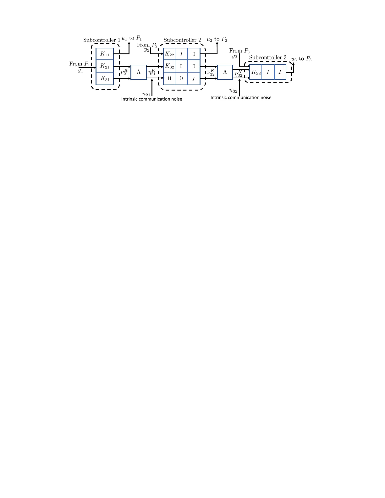
1 A Y oula Operator State-Space Frame work for Stably Realizable Distrib uted Control Mohammad Naghnaeian, Petros G. V oulgaris, and Nicola Elia Abstract —This paper deals with the pr oblem of distributed control synthesis. W e seek to find structur ed controllers that are stably realizable over the underlying network. W e address the problem using an operator f orm of discrete-time linear systems. This allows f or uniform tr eatment of various classes of linear systems, e.g., Linear Time In variant (L TI), Linear Time V arying (L TV), or linear switched systems. W e combine this operator repr esentation f or linear systems with the classical Y oula parameterization to characterize the set of stably realizable controllers for a given network structure. Using this Y oula Operator State-Space (YOSS) framework, we show that if the structure satisfies certain subspace like assumptions, then both stability and performance pr oblems can be formulated as con vex optimization and more precisely as tractable model-matching problems to any a priori accuracy . Furthermore, we show that the structured controllers found from our appr oach can be stably realized over the network and provide a generalized separation principle. I . I N T R O D UC T I O N Modern large-scale cyber-physical systems are composed of many interconnected subsystems that are usually spread ov er a large geographic area and communicate over a network. Many difficulties arise when designing a centralized controller for such systems due to communication delays, the structure of the underlying communication network, scalability , etc. Due to these issues, there has been a shift tow ards designing decen- tralized controllers, in which subcontrollers are designed and implemented for each subsystem and they can communicate ov er the netw ork. Decentralized, structured and distrib uted controller design has attracted the renewed attention of many researchers over the last 15 years or so. Several new de velopments occurred using state space methods (e.g., in the LMI frame work [1], [2]) which suit quadratic criteria but could generally lead to suboptimal solutions. On the other hand, input-output approaches using the Y oula-parametrization were found to be very powerful in pro viding truly optimal solutions for several classes of structured problems by reducing them to conv ex problems o ver the Y oula parameter, encompassing a variety M. Naghnaeian is with the Mechanical Engineering Department, Clemson Univ ersity , Clemson, SC, USA mnaghna@clemson.edu P . G. V oulgaris is with the Aerospace Engineering Department and the Coordinated Science Laboratory , University of Illinois, Urbana, IL, USA voulgari@illinois.edu , and Aerospace Engineering Department, Khalifa Uni versity , Abu Dhabi, U AE petros.voulgaris@kustar.ac.ae N. Elia is with the Department of Electrical Engineering, Iowa State Univ ersity , Ames, IA 50010 USA nelia@iastate.edu This work is partially supported by NSF awards CMMI-1663460, ECCS- 1739732, CCF-1717154, CIF-1220643, and AFOSR AF F A-9550-15-1-0119 of criteria, including nonquadratic (e.g., [3], [4], [5], [6], [7],[8],[9]). In the input-output, or transfer function, domain, the sta- bilizing controllers are parametrized by the so-called Y oula parameter , and the search for the optimal Y oula parameter is carried out ov er the space of stable systems. Here, the order of the Y oula parameter or that of the controller is not assumed a priori. Ho we ver , unlike the state-space approaches, the realizability of the controller o ver the underlying commu- nication network may become an issue, if not taken directly into account as pointed out in [10], [11]. That is, although the controller transfer function structure is compatible with the underlying network communication graph, it may lead to an internally unstable realization, i.e., a non-minimal realization with unstable pole zero cancellations (e.g., [12], [13] and [14]). Certain alternativ e input-output approaches have recently been proposed (e.g., a system le vel approach in [15] and references therein) that hold the potential to handle certain optimal and stably realizable structured design, by conv ex programming without resorting to Y oula-parametrization. A potential draw- back is the need to solve an exact model-matching problem, i.e., equations that, if possible to satisfy , may require infinite support of the L TI maps in volv ed and hence stopping criteria for the approximation by finite support may not be precisely characterized. In this paper, we propose a unified way to synthesize stably realizable controllers with respect to any measure of performance, e.g., l 1 , l 2 , or l ∞ induced norms. Our approach is based on utilizing a state-space based operator form of the system and combining it with the ideas in the Y oula- parameterization. This has been dev eloped initially in the context of switching system analysis and design in [16], [17], and as it turns out, it fits well for optimally solving structured problems [18]. Our approach in volves revisiting classical rob ust control problems, e.g. H ∞ or l 1 , and proposing a new way to check for stability and to parametrize the set of stabilizing controllers. The stability check that we will develop in this paper is in the form of a model-matching problem inf R stable. k T 1 + T 2 RT 3 k , where T 1 , T 2 , and T 3 are stable systems. Such problems are conv ex and efficient algorithms exist to solve them with arbitrary accuracy . As such, we depart from standard stability tests, e.g., eigen value or quadratic L yapunov results. This will allow us to propose a new way to parameterize the set of all stabilizing controllers, which is especially beneficial to designing decentralized controllers with stable realization. 2 Another nov elty of this approach is a new separation principle. Although the standard separation principle does not generally hold true in the context of decentralized control, this newly formulated separation principle holds v alid. In order to present this new separation principle, first, we introduce the class of full-information-like controllers. These are controllers that map both the state and measured output to control input. That is, u =  K 1 K 2   x y  , (1) where u , x , and y are control input, states, and measured output, respectiv ely; K 1 and K 2 are linear systems. The proposed separation principle states that any full-information- like controller (1) yields an output feedback controller if x is replaced by its estimation ˆ x , which in turn is generated by an observer from the measured output. Furthermore, although the reader can focus on the L TI case as a concrete example, these methods are general and hold for L TV , delayed, and switching systems as well. I I . P R E L I M I N A R I E S In this paper , R and Z denote the sets of real numbers and integers, respectively . The set of n -tuples x = { x ( k ) } n − 1 k =0 where x ( k ) s are real numbers is denoted by R n . For any x ∈ R n , its l ∞ and l p norms are defined as k x k ∞ = max k ∈{ 0 , 1 ,...,n − 1 } | x ( k ) | and k x k p =  P n − 1 k =0 | x ( k ) | p  1 p , respectiv ely . Let g = { g ( k ) } ∞ k =0 be a sequence where g ( k ) ∈ R n . Then, the l ∞ and l p norm of this sequence are defined as k g k ∞ = sup k ∈ Z + k g ( k ) k ∞ and k g k p =  P ∞ k =0 k g ( k ) k p p  1 p whenev er they are finite. The set of R n -valued sequences whose l p norm ( l ∞ norm) is finite is denoted by l n p ( l n ∞ ). Giv en two normed spaces ( X , k . k X ) and ( Y , k . k Y ) and a linear operator T : X → Y , its induced norm is defined as k T k X − Y := sup f 6 =0 k T f k Y k f k X . Whene ver both v ector spaces are X , we use the notation k T k without any subscript if the result holds for any induced norm. W e will call T bounded or stable if || T || < ∞ . Any linear causal map T , on the space of all sequences ( l ∞ ,e ), can be thought of as an infinite dimensional lower triangular matrix, T =    T 0 , 0 0 · · · T 1 , 1 T 1 , 0 · · · . . . . . . . . .    . (2) Such a causal map T is called strictly causal if its diagonal elements are zeros, i.e., T 0 , 0 = T 1 , 0 = ... = 0 . W e say T is a squar e operator if it has the same number of inputs as outputs, that is, T i,j terms are square matrices. Given a sequence g = { g ( k ) } ∞ k =0 , the delay or shift operator Λ is defined by Λ k g =    0 , ..., 0 | {z } k zeros , g (0) , g (1) , ...    , and, with a slight abuse of notation, Λ − k g = { g ( k ) , g ( k + 1) , ... } . It is easy to show that if T is a causal map then Λ T and T Λ are strictly causal. Con versely , any strictly causal operator T can be written as T = Λ ¯ T where ¯ T is causal. A linear causal map T is called time-in variant if it commutes with the delay operator , i.e. Λ T = T Λ . If T is a Linear Time-In variant (L TI), it is fully characterize by its impulse response denoted by { T ( k ) } ∞ k =0 . In this case, its infinite dimensional matrix representation is gi ven by T =    T (0) 0 · · · T (1) T (0) · · · . . . . . . . . .    . A finite dimensional L TI system has the state-space represen- tation of G :  x ( t + 1) = Ax ( t ) + B u ( t ) y ( t ) = C x ( t ) + D u ( t ) , with x ( t 0 ) = x 0 , (3) where u ( t ) ∈ R m , x ( t ) ∈ R n , y ( t ) ∈ R p , and x 0 ∈ R n are input, state, output, and the initial condition of the system and A , B , C , and D are matrices with appropriate dimensions for all t ∈ Z + . Given a matrix S , we define ˆ S to be the diagonal operator ˆ S =    S 0 · · · 0 S . . . . . .    . (4) Using this notation, we can define diagonal operators ˆ A , ˆ B , ˆ C , and ˆ D and rewrite (3) as G :  x = Λ ˆ Ax + Λ ˆ B u + ¯ x 0 y = ˆ C x + ˆ D u , (5) where ¯ x 0 =    0 , ..., 0 | {z } t 0 zeros , x 0 , 0 , 0 , ...    , x = { x ( t ) } ∞ t =0 , y = { y ( t ) } ∞ t =0 , u = { u ( t ) } ∞ t =0 , and Λ is the delay operator . The abov e representation of G is referred to as a realization in operator form. One can also write an operator realization for the time delay systems. Consider the system gi ven by H : ( x ( t + 1) = P N i =0 A i x ( t − i ) + P N i =0 B i u ( t − i ) y ( t ) = P N i =0 C i x ( t − i ) + P N i =0 D i u ( t − i ) , (6) with initial condition x 0 = { x ( k ) } 0 k = − N . Define ¯ A = P N i =0 Λ i ˆ A i . Similarly , we define ¯ B , ¯ C , and ¯ D . Then, the time- delay system can be written in the operator form as H :  x = Λ ¯ Ax + Λ ¯ B u + ¯ x 0 y = ¯ C x + ¯ D u . (7) In this operator framew ork, we make a distinction between an operator and its realization as follows: Definition 1 (Operator Realization): For a giv en linear (possibly unbounded) causal operator T : u → y , we will refer to the relationship T :  x = A T x + B T u y = C T x + D T u , as an operator realization or simply a realization only if operators A T , B T , C T , and D T are bounded causal operators and ( I − A T ) − 1 exists. 3 For example, realizations for L TI operators (3) and delayed systems (6) are given in (5) and (7), respecti vely . Also, any bounded operator T has a trivial realization with A T = B T = C T = 0 and D T = T . This realization, howe ver , is not tri vial for unstable operator T . Throughout this paper , we prefer to write the systems in the operator form (7) as it allows for treating various classes of systems (e.g. time-delay , switching, and L TV systems [16]) in a unified way . Henceforth, we consider the systems that hav e operator forms as in (7). Such a system can be seen as a mapping from ¯ x 0 and u to x and y . For this system, we adopt the follo wing definitions of stability and gain. Definition 2: Giv en two normed spaces ( U , k . k U ) and ( X , k . k X ) , we say that the system H in (7) is U to X stable if it is a bounded operator from  ¯ x T 0 , u T  T ∈ X × U to  x T , y T  ∈ X × X . More precisely , H is U to X stable if, for some γ 1 , γ 2 ≥ 0 , k x k X ≤ γ 1 k ¯ x 0 k X + γ 2 k u k U and k y k X ≤ γ 1 k ¯ x 0 k X + γ 2 k u k U whenev er k ¯ x 0 k X and k u k U are finite. Definition 3: Giv en two normed spaces ( U , k . k U ) and ( X , k . k X ) , and a U to X stable system H , its gain is defined as k H k U −X = sup u 6 =0 x 0 =0 k y k X k u k U . For simplicity , we let X and U to be the same (but possibly with dif ferent dimension) l p spaces. Finally , when need to ensure the in vertibility of certain operators on l ∞ ,e , we will appeal to the following lemma: Lemma 1: The following hold: 1) Giv en a causal square operator T as in (2), the inv erse ( I − T ) − 1 exists if T i, 0 is in vertible for all i = 0 , 1 , 2 , ... . 2) Giv en a partitioned squared operator X =  X 11 X 12 X 21 X 22  , ( I − X ) − 1 exists if ( I − X 11 ) and ( I − X 22 ) are in- vertible. I I I . B A S I C S E T U P A standard practice for designing a distributed controller for subsystems communicating ov er a given network is to aggregate all subsystems into one system P and design a controller for this system. The controller must be designed in a way so that it can be implemented as subcontrollers communicating o ver the giv en network. W e consider the aggregate system with a realization P :    x = Λ ¯ Ax + Λ ¯ B 1 w + Λ ¯ B 2 u + ¯ x 0 z = ¯ C 1 x + ¯ D 11 w + ¯ D 12 u y = ¯ C 2 x + ¯ D 12 w , , (8) where x, y , and z are the states, measurements, and the regulated output; w and u are the exogenous and control inputs; and, ¯ A, ¯ B i , ¯ C j , ¯ D ij , for i.j ∈ { 1 , 2 } are bounded operators. Example 1: Consider a network with N subsystems. Each subsystem is gi ven by x i ( t + 1) = A i x i ( t ) + B i 1 w i ( t ) + B i 2 u i ( t ) + N X j =1 B ij 3 η ij ( t ) , z i ( t ) = C i 1 x i ( t ) + D i 11 w i ( t ) + D i 12 u i ( t ) , y i ( t ) = C i 2 x i ( t ) + D i 21 w i ( t ) , ν j i ( t ) = C j i 3 x i ( t ) + D j i 31 w i ( t ) , j = 1 , 2 , ..., N , (9) where x i , y i , and z i are the states, measured output, and regulated output of the i th subsystem; ν j i is the signal that the i th subsystem communicates to the j th subsystem and η ij is the signal that i th subsystem receives through its communication link with the j th subsystem. W e let B ij 2 = C j i 3 = D j i 31 = 0 if there is no communication link between i th and j th subsystems. Furthermore, due to the delay in the communication links, we set η ij ( t ) = ν ij ( t − τ ij ) , (10) where τ ij ∈ Z ≥ 0 is delay in communication from j th to i th subsystem. Substituting (10) in (9), the i th subsystem, in the operator form, can be written as x i = Λ   ˆ A i x i + 3 X j =1 Λ τ ij ˆ A ij x j   +Λ   ˆ B i 1 w i + 3 X j =1 Λ ij ˆ B ij 1 w j   + Λ ˆ B i 2 u i , where ˆ A ij = ˆ B ij 3 ˆ C ij 3 and ˆ B ij 1 = ˆ B ij 3 ˆ D ij 31 . Based on the above expression, it can be easily seen that for properly defined operators ¯ A, ¯ B i , ¯ C i , ¯ D ij , for i ∈ { 1 , 2 } , the aggregate system can be written as in (8). The structure of the network is reflected in the coefficient operators in volved in (8), e.g., as sparsity patterns [14]. Giv en a fixed network consisting of N nodes (subsystems) and a set of N inputs ξ = [ ξ i ] to, and N outputs ζ = [ ζ i ] from, these N nodes, let S denote the set of all input-output maps (or , transfer functions in the L TI case) T from ζ to ξ , i.e., ξ = T ζ that can be obtained from this network. That is, the input-output aggregation of all subsystem (or , subcontroller) dynamics, interconnected via the network, form an element T in S and, conv ersely , any element in S can be implemented, stably or unstably (to be precisely defined later), as subsystems communicating o ver the gi ven network. Consider the following example: Example 2: Nested network: An example of a nested net- work is giv en in Figure 1. W e adopt the notations introduced in Example 1. It can be easily verified that the aggregate system is gi ven by (8) where ¯ A =  ¯ A (0) , ¯ A (1) , 0 , 0 , ...  , ¯ B 1 =  ¯ B 1 (0) , ¯ B 1 (1) , 0 , ...  , ¯ B 2 =  ¯ B 2 (0) , 0 , ...  , ¯ C j =  ¯ C j (0) , 0 , ...  , ¯ D ij =  ¯ D ij (0) , 0 , ...  with ¯ A (0) = diag  A 1 , A 2 , A 3  , ¯ B j (0) = diag  B 1 j , B 2 j , B 3 j  , ¯ C j (0) = 4 ? 6 P 1 - 6 P 2 P 3 - 6 Λ Λ ? ? 6 6 u 1 u 2 u 3 y 1 w 1 z 1 w 2 w 3 y 2 y 2 z 2 z 2 ν 21 η 21 ν 32 η 32 Fig. 1. A simple nested network. diag  C 1 j , C 2 j , C 3 j  , ¯ D ij (0) = diag  D 1 ij , D 2 ij , D 3 ij  , and for i, j ∈ { 1 , 2 } ¯ A (1) =   0 0 0 B 21 3 C 21 3 0 0 0 B 32 3 C 32 3 0   , ¯ B 1 (1) =   0 0 0 B 21 3 D 21 31 0 0 0 B 32 3 D 32 31 0   . In this example, the structure of the network is reflected on the impulse response of the coefficient operators, e.g. ¯ A . The terms in the impulse response of ¯ A are lower triangular , which conforms with the flo w of communication from subsystem 1 to subsystem 2 and then to subsystem 3 . And the sparsity structure in ¯ A (0) and ¯ A (1) is because each subsystem has immediate access to its own measurement signal but commu- nicates with its neighbors with a delay . For this network, the set S is the space of all systems P whose impulse response { P ( k ) } ∞ k =0 satisfies the following conditions: P ( k ) is lower triangular for k = 2 , 3 , ... , P (0) is diagonal, and P (1) =   ∗ 0 0 ∗ ∗ 0 0 ∗ ∗   , where ∗ stands for a possibly non zero entry . Or , in transfer function terms, P [ λ ] =   ∗ 0 0 λ ∗ ∗ 0 λ 2 ∗ λ ∗ ∗   , where P [ λ ] = P ∞ k =0 λ k P ( k ) is the λ -transform. Accordingly , if K is a controller for P within the same communication network, K [ λ ] should also be of the same form, i.e., K ∈ S . In the sequel, in generating the control input u , depending on what information is av ailable, we face two categories of problems, full-information or output feedback. In full- information feedback, the controller has access to the entire state and measured outputs, i.e., u =  K 1 K 2   x y  . (11) In output feedback, ho we ver , u must be generated only using the information a v ailable in signal y , i.e. u =  0 K 2   x y  . Remark 1: W e need to point out that there is a dif ference between the full-information controller that we defined in (11) and the one defined in [19]. In the latter , the controller has access to the state x and the disturbances w (and consequently y ) while the full-information controller defined in (11) only has access to x and y . The two definitions are equiv alent if ¯ D 21 is a square and in vertible map. The generalized plant  x y  =  Λ ¯ A 0 ¯ C 2 0   x y  +  Λ ¯ B 1 w + Λ ¯ B 2 u + ¯ x 0 ¯ D 21 w  , z =  ¯ C 1 0   x y  + ¯ D 11 w + ¯ D 12 u, (12) with the full-information feedback controller (or output feed- back when K 1 = 0 ) results in the closed-loop system  x y  =  I − Λ ¯ A − Λ ¯ B 2 K 1 − Λ ¯ B 2 K 2 − ¯ C 2 I  − 1 ×  Λ ¯ B 1 ¯ D 21  w +  I 0  ¯ x 0  , z =  ¯ C 1 0   x y  + ¯ D 11 w + ¯ D 12 u, u =  K 1 K 2   x y  . (13) This closed-loop system can be thought of as a linear oper- ator from  ¯ x 0 w  to signals x , y , z , and u . In conjunction with Definition 2, we adopt the following definition for centralized stabilizing controllers Definition 4 (Centralized Stabilizing Structur ed Contr oller): A full-information or output feedback structured controller K =  K 1 K 2  ∈ S 1 × 2 is said to be stabilizing in the centralized way if the closed loop system (13) is a bounded operator from ¯ x 0 and w to x , y , z , and u . It is important to note that an implementation of a controller in a distributed way ov er a network is carried out through implementing a realization of such controller that conforms with the network structure. Howe ver , unless K ∈ S is a bounded operator itself, there is no apriori guarantee that it has an operator realization conforming with the structure of the network. In the next subsection, we will discuss this issue further . A. Stable r ealizability/implementability The set S is fully characterized by the underlying network. In this paper , giv en a (stabilizable and detectable in the usual sense) generalized plant P =  P z w P z u P y w P y u  as in (8), we are interested in finding the controllers K ∈ S that are also stably realizable ov er the network. W e should point out that e ven if K belongs to S and stabilizes P in the usual centralized sense (Definition 4), i.e., if  I P y u K I  (14) has a stable in verse, it does not mean that the controller K can automatically be realized stably , although we can implement 5 In t r i n s i c c o mmu n i c a t i o n n o i s e In t r i n s i c c o mmu n i c a t i o n n o i s e Fig. 2. Controller in Example 3 implemented over the network. it as the interconnection of subcontrollers consistent with the network. Unless we guarantee that the implementation of K does not hav e internal hidden unstable modes, the closed-loop may not be stable. This is because a stabilizing controller in a centralized sense, by design, guarantees the boundedness (stability) of the measured output and control input, y and u . Also, under the detectability assumption of the plant, the boundedness of y and u translates to that of x and z in (8). Howe ver , when an aggregate controller is implemented in a decentralized way , new signals are introduced and should taken into consideration. In particular , these are the signals trav elling between subcontrollers and also the intrinsic noise on such signals. Therefore, in designing a controller that is implementable over the network in a stable way , one needs to identify the subcontrollers’ communication signals and guarantee that the effects of their intrinsic noise on ev ery other signal of the system is bounded. Example 3: Consider the nested network in Example 2 and let K ∈ S be a stabilizing controller in the centralized sense as in (14). Since K = { K ( k ) } ∞ k =0 ∈ S , it can be partitioned as K =   K 11 0 0 Λ K 21 K 22 0 Λ 2 K 31 Λ K 32 K 33   . One way to implement this controller over the network is illustrated in Figure 2. By definition, the signals y , z , and u are bounded when w and ¯ x 0 are bounded. Howe ver , as mentioned above, it is not guaranteed that the signals trav elling between the subcontrollers, i.e. ν K 21 and ν K 32 , are bounded. Furthermore, it is not clear if small bounded noise signals, shown as n 21 and n 32 in the figure, corrupt the subcontrollers’ communications, the stability of the system, i.e., the boundedness other signals is preserved. of Therefore, special attention should be paid to the stable implementability of structured controllers. Accordingly , we define the set S K ⊆ S to be the set of stabilizing controllers K that can be stably implemented over the network without loosing stability , i.e., the subcontrollers communicate bounded signals provided that the measured outputs, y , and control inputs, u , are bounded. W e will make the definition of S K concrete in what follows. Definition 5 (Stably Realizable Contr oller ): Giv en a struc- tured aggregate controller K =  K 1 K 2  ∈ S 1 × 2 ( K 1 = 0 for output feedback) that is centralized stabilizing in the sense of Definition 4, we say K is stably realizable ov er the structure S , i.e., K ∈ S K if the follo wing two conditions hold: 1) It has an operator realization K :  x K = A K x K + B K ¯ y u = C K x K + D K ¯ y , (15) where a) for full-information feedback ¯ y =  x T , y T  T and A K ∈ S m × m , B K ∈ S m × 2 , C K ∈ S 1 × m , D K ∈ S 1 × 2 , b) and for output feedback ¯ y = y , A K ∈ S m × m , B K ∈ S m × 1 , C K ∈ S 1 × m , D K ∈ S 1 × 1 , for some positive integer m and stable operators A K , B K , C K , and D K . 2) The effects of fictitious subcontrollers’ communication noise, denoted by n x and n u , on the system is bounded. That is, the interconnection of ”noisy controller” ¯ K :  x K = A K x K + B K ¯ y + n x u = C K x K + D K ¯ y + n u , (16) and the plant P in (8) results in a bounded closed-loop operator from ¯ x 0 , w , n x , and n y to x , y , x K , and u . W e refer to (15) as a stable realization or implementation of the controller K . Giv en S , it is not clear that every centralized stabilizing controller (in the sense of Definition 4), K ∈ S , can be stably realized ov er the network structure. Therefore, we always have S K ⊆ S . In this paper, given a structure S , we dev elop necessary and suf ficient conditions in terms of conv ex problems under which it is possible to find optimal structured controllers K ∈ S K that are stably implementable over the network. A typical S of interest consists of controllers with certain sparsity or delay patterns. Furthermore, we assume that S is a subspace that satisfies the following: Assumption 1: The set S is delay-in variant, contains identity and zero, and is closed under addition and multiplication, i.e., I , 0 ∈ S , Λ S ∈ S and for any X , Y ∈ S , X + Y ∈ S and X Y ∈ S . Assumption 2: The set S contains the coef ficient operator ¯ A , ¯ B 2 , and ¯ C 2 . Under such assumptions, as we will show S K = S . In addition to the above assumption, we make the following 6 assumption pertaining to the fact that all of the measured outputs, y , are corrupted by noise. Assumption 3: ¯ D 21 has a tri vial left null space. I V . Y O U L A O P E R A T O R S TA T E - S P AC E P A R A M E T R I Z A T I O N O F S TA B I L I Z I N G C O N T R O L L E R S In this section, we re visit a classical robust result on parametrizing the set of stabilizing controllers. Traditionally , a typical approach to find the set of stabilizing controllers is via Y oula-Kucera parametrization that utilizes the doubly coprime factorization. Here, we propose a new approach in the operator framework that do not require coprime factorization. This approach is referred to as the Y oula Operator State-Space (Y OSS) and proves to be particularly powerful in designing decentralized controllers for linear systems. A. YOSS for Full-Information F eedback For the full-information feedback problems, we first parametrize the set of all centralized stabilizing structured controllers in the sense of Definition 4. And then, we will show ho w such controllers can be stably realized/implemented in a distributed way ov er the network structure in the sense of Definition 5. In order to state the result, we define an affine expression E Q,Z in terms of bounded operators Q and Z as follows: E Q,Z :=  Λ ¯ A 0 ¯ C 2 0  +  Λ ¯ A − I 0 ¯ C 2 − I  Q +  Λ ¯ B 2 0  Z. (17) Then, the follo wing theorem holds: Theor em 1: The following conditions are equi valent: 1) There exists a centralized stabilizing structured full- information feedback controller K ∈ S :  x T , y T  T → u for the the plant (12). 2) There exist stable causal operators Q and Z and some ε ∈ [0 , 1) such that: a) Model-Matching: kE Q,Z k ≤ ε. (18) b) Structure: Q and Z can be partitioned as Q =  Λ Q 11 Λ Q 12 Q 21 Λ Q 22  , Z =  Z 1 Z 2  , Q i,j ∈ S , Z i ∈ S for i, j = 1 , 2 . (19) 3) For any ε ∈ [0 , 1) , there exist stable causal operators Q ε and Z ε such that Conditions 2.a and 2.b hold for Q = Q ε and Z = Z ε . 4) There exist stable causal operators Q 0 and Z 0 such that Conditions 2.a and 2.b hold for ε = 0 , Q = Q 0 , and Z = Z 0 . Cor ollary 1: Gi ven a centralized full-information feedback controller K ∈ S 1 × 2 , there exists stable operators Q and Z such that (18) and (19) hold for some ε ∈ [0 , 1) and K can be decomposed as K =  K 1 K 2  = Z ( I + Q ) − 1 , (20) where the in verse ( I + Q ) − 1 exists by Lemma 1. Theorem 1 pro vides a con vex way to parametrize the set of all centralized stabilizing controllers that have the structure. Furthermore, Corollary 1 provides a factorization for the controller that can be used to obtain an operator realization for the controller . T o this end, note that according to (20) u = Z ( I + Q ) − 1  x T , y T  T . Defining x K = ( I + Q ) − 1  x T , y T  T , a full-information controller can be realized as K :  x K = A K x K + B K ¯ y u = C K x K + D K ¯ y , (21) where ¯ y =  x T , y T  T and A K = − Q ∈ S 2 × 2 , B K = I 2 × 2 ∈ S 2 × 2 , C K = Z ∈ S 1 × 2 , D K = 0 1 × 2 ∈ S 1 × 2 , with Q and Z satisfying (18) for some ε ∈ [0 , 1) . This is an operator realization of the controller that conforms with the network structure. In order to sho w that this realization provides a stable implementation, in the sense of Definition 5, we need to show that the noisy version of such a controller with fictitious subcontrollers’ communication noise as giv en in (16) results in a bounded closed-loop map. Theor em 2: Any centralized stabilizing full-information controller with structure can be stably realized over the net- work structure through realization (21). That is, S K = S . According to Theorem 1, parametrizing the set of all full-information stabilizing controllers amounts to solving an optimization problem (18) over the space of stable operators ( Q, Z ) for some giv en ε ∈ [0 , 1) . Such optimization problems are in the generic form inf R k T 1 + T 2 RT 3 k , where T 1 , T 2 , T 3 , and R are stable operators. This optimization, which is commonly referred to as a model-matching problem in robust control community , is con vex and there are efficient methods to solve it with arbitrary accuracy . In particular , when the operator norm is taken to be the l ∞ induced norm, this optimization can be cast as a linear program. Remark 2: According to Theorem 1, although the model- matching (18) can be carried out with ε = 0 , it is advanta- geous, for computations, to relax the condition to ε ∈ [0 , 1) as stated in the theorem. As a matter fact, if ε is set to zero, there might not exist any finite-impulse response Q and Z that satisfy (18). For example, consider a tri vial uncontrollable but stable system x ( t + 1) = 1 2 x ( t ) + w ( t ) + 0 u ( t ) , y ( t ) = x ( t ) + w ( t ) . Then, it can be easily verified that Q =  Λ Q 11 0 I + Λ Q 11 0  , and any stable Z satisfy (18) for ε = 0 if and only if Q 11 has the impulse response n 1 2 ,  1 2  2 ,  1 2  3 , ... o . This is particularly important since the approximation with FIR will fail to provide performance guarantees. 7 B. YOSS for Output F eedback The output feedback controllers form a subset of full- information feedback controllers, which were parametrized in Theorem 1 and Corollary 1. More precisely , a full-information controller (20) is an output feedback controller if K 1 = 0 or equiv alently Z ( I + Q ) − 1  I 0  = 0 . (22) Therefore, we ha ve the following theorem. Theor em 3: The following conditions are equi valent: 1) There exists a centralized stabilizing output-feedback controller K : y → u . 2) There exist stable causal operators Q and Z and some ε ∈ [0 , 1) such that (18)-(19) and (22) hold. 3) For any ε ∈ [0 , 1) , there exist stable causal operators Q ε and Z ε such that Condition 2 holds for Q = Q ε and Z = Z ε . 4) There exist stable causal operators Q 0 and Z 0 such that (18), (19), and (22) hold for Q = Q 0 , Z = Z 0 , and ε = 0 . If any of the abov e equi v alent conditions hold, a stabilizing output-feedback controller K : y → u is giv en by K = Z ( I + Q ) − 1  0 I  . Although finding the set of stabilizing full-information feedback controllers, as gi ven in Theorem 1, is a con vex and tractable problem, this is not the case for output feedback due to the non-con vexity associated with (22). W e emphasize that (22) is enforced to restrict the set of full-information stabilizing controllers, u =  K 1 K 2   x y  , to the ones whose K 1 element is zero. In what follows, we will relax condition (22), in order to preserve the con vexity , and will replace x with its estimation ˆ x , which is generated based on y , in order to preserve the output feedback structure. More precisely , we will consider controllers of the following form u =  K 1 K 2   ˆ x y  , where ˆ x is an estimation of x generated from observing y and u such that the estimation error, e = ˆ x − x , is a bounded signal. The estimation ˆ x is generated by an state-estimator in the follo wing generic form ˆ x = E 1 u + E 2 y , (23) where E 1 and E 2 are causal operators. Later (in Theorem 5), we will sho w that there alw ays e xist bounded operators E 1 and E 2 conforming with the network structure, i.e., E 1 , E 2 ∈ S . Theor em 4: Suppose ˆ x is a an estimation of x generated via the generic estimator (23) such that E 1 , E 2 ∈ S and k e k ≤ δ for some δ > 0 , where e = ˆ x − x . Then, the following conditions are equi valent: 1) A structured output-feedback controller ˜ K ∈ S : y → u is stabilizing when implemented in the centralized way . 2) There exists causal operators K 1 , K 2 ∈ S such that u =  K 1 K 2   ˆ x y  = ˜ K y . (24) 3) There exist stable causal operators Q and Z and some ε ∈ [0 , 1) such that  K 1 K 2  = Z ( I + Q ) − 1 , (25) and Q and Z satisfy: a) Model-Matching (18) holds. b) Structure constraints (19) are satisfied. 4) For any ε ∈ [0 , 1) , there exist stable causal operators Q ε and Z ε such that Condition 3 holds for Q = Q ε and Z = Z ε . In the light of this theorem, the parametrization of all stabilizing output feedback controllers can be carried out via a conv ex search ov er parameters ( Q, Z ) provided that an estimation ˆ x of the states x with uniform bound, k ˆ x − x k ≤ δ , is av ailable, which is the subject of next section. By uniformity we mean that the bound δ does not depend on the control input u and is uniform with respect to w and ¯ x 0 . More precisely , the should exist δ 1 , δ 2 ≥ 0 such that k e k ≤ δ 1 k ¯ x 0 k + δ 2 k w k . The parametrization presented here does not require the doubly coprime factorization of the plant and this is an advantage especially when designing decentralized controllers. Further- more, this parameterization holds valid not only for L TI systems but also any other linear system, e.g., delayed , time- varying, or switching systems. 1) State-Estimator: Here, we will define an state-estimator that mimics the standard Luenberger observer with a dif ference that its observer gain is a possibly unbounded operator . This state-estimator is referred to as the Generalized Luenber ger Observer and has the form ˆ x = Λ ¯ A ˆ x + Λ ¯ B 2 u + Λ L  ¯ C 2 ˆ x − y  , (26) where L is the observer operator-g ain which can possibly be unstable. Theor em 5: If there exists a centralized stabilizing output feedback controller with structure, there always exists a gen- eralized Luenberger observer (26) with the network structure. The observer operator-gain is given by L = ( I + Q ε L Λ) − 1 Z ε L ∈ S (27) where, for any ε ∈ [0 , 1) , Q ε L ∈ S and Z ε L ∈ S are stable causal operators satisfying kE L k ≤ ε , where E L := ¯ A + Z ε L ¯ C 2 − Q ε L  I − Λ ¯ A  . (28) In this case, the state-estimator is simplified to ˆ x = R 1 Λ ¯ B 2 u − R 2 y , (29) where R 1 :=  I − Λ  ¯ A + L ¯ C 2  − 1 ∈ S , (30) and R 2 := R 1 Λ L ∈ S , (31) 8 are bounded operators. Furthermore, the estimation error e is giv en by e = ˆ x − x = −  R 1 Λ ¯ B 1 + R 2 ¯ D 21  w − R 1 ¯ x 0 . (32) A realization of the state-estimator is giv en by (28) and can also be re written as ˆ x = Λ E L ˆ x + ( I + Λ Q ε L ) Λ ¯ B 2 u − Λ Z ε L y . (33) 2) Stable Realization of Output F eedback: The operator forms (25) and (33) provide basis for stable realization of the ov erall controller ov er the network. The controller (25) can be realized as  ξ 1 ξ 2  = −  Λ Q 11 Λ Q 12 Q 21 Λ Q 22   ξ 1 ξ 2  +  ˆ x y  , u =  Z 1 Z 2   ξ 1 ξ 2  . (34) Then, combining the realization of the state-estimator (33) with (34), we obtain the following realization for the output feedback controller K : y → u : K :  x K = A K x K + B K y u = C K x K , (35) where A K =   Λ E L ( I + Λ Q ε L ) Λ ¯ B 2 Z 1 ( I + Λ Q ε L ) Λ ¯ B 2 Z 2 I − Λ Q 11 − Λ Q 12 0 − Q 21 − Λ Q 22   , B K =   − Λ Z ε L 0 I   , C K =  0 Z 1 Z 2  . (36) In the abov e expression, x K is given by x K =  ˆ x T , ξ T 1 , ξ T 2  T , where ˆ x is the state-estimator as gi ven in (33) and ξ 1 and ξ 2 are the signals giv en in (34). The realization (35) is implementable ov er the network as operators A K , B K , and C K conform with the network structure S 1 . W e, howe ver , need to show that such implementation is stable. That is, the stability of the system is preserved even if the signals trav eling between the subcontrollers are subject to noise, that is, if the noisy controller ¯ K :  x K = A K x K + B K y + n x u = C K x K + n u (37) is implemented. In other words, we need to show that the closed-loop maps from subcontrollers communication noise n x and n u to signals x , y , u , and x K are bounded. Theor em 6: The realization giv en in (35) can be imple- mented stably over the giv en network structure S . That is, the feedback interconnection of ¯ K and the plant results in bounded signals x , y , x K and u . This is , S K = S . 1 For sparsity structures, one can find the realization of each subcontroller, from the realization of the aggregate controller , using a procedure similar to that of [9]. V . O P T I M A L C O N T R O L S Y N T H E S I S In the last section, we parametrized the set of all structured stabilizing controllers via a conv ex model-matching problem (18) while enforcing the netw ork structure on components of Q and Z as in (19) . These conditions are identical for full- information and output feedback controllers. Furthermore, a stable realization for stabilizing controllers was gi ven as in (21) for full-information feedback and (35) for output feedback controller . This subsection is de voted to finding the optimal controller such that the closed-loop gain from the exogenous input w to regulated output z is minimized. T o this end, first, we will derive the set of all closed-loop maps from w to z when an output stabilizing controller is utilized. The set of all output stabilizing controllers is parametrized by Theorem 4. For fixed ε ∈ [0 , 1) , the set of all such controllers are giv en by u = Z ( I + Q ) − 1  ˆ x y  , (38) where ( Q, Z ) satisfies (18)-(19) and ˆ x is an state estimation. First, we find and fix a state-estimator (33) with structure as in Theorem 5. The the following holds: Pr oposition 1: The generalized plant (12) with the output feedback controller (38) results in the follo wing closed-loop map Φ wz from w to z : Φ wz = H + U  Q Z  V + U  I + Q Z  E ( I − E ) − 1 V , (39) where E = E Q,Z giv en in (17), H = ¯ C 1 Λ ¯ B 1 + ¯ C 1 Λ ¯ A  R 1 Λ ¯ B 1 + R 2 ¯ D 21  + ¯ D 11 , (40) U =   ¯ C 1 0  ¯ D 12  , (41) V =  Λ ¯ B 1 ¯ D 21  +  Λ ¯ A − I ¯ C 2   R 1 Λ ¯ B 1 + R 2 ¯ D 21   , (42) with R 1 and R 2 being stable operators defined in (30)-(31). Notice that E as defined in (17) can be made arbitrarily small according to Theorem 4. Therefore, without loss of generality , one can set E in (17) equal to zero; in which case, the closed- loop map Φ wz will be an affine function of stable operators Q and Z . This is stated in the follo wing theorem without any further proof: Theor em 7: Given a fixed generalized Luenberger observer , as provided in Theorem 5, any stably realizable output feed- back controller can be written as a mapping from state- estimator ˆ x and measured output y to control input u , i.e., K :  ˆ x y  → u , in the form (38),where ( Q, Z ) satisfies (18)- (19) for ε = 0 . Then, the closed-loop norm from the e xogenous input w to regulated output z is gi ven by Φ wz ( K ) = H + U  Q Z  V . Furthermore, the optimal achiev able closed-loop gain, i.e., γ opt := inf K ∈S stabilizing k Φ wz ( K ) k , is giv en by γ opt = inf Q,Z ∈S     H + U  Q Z  V     , 9 subject to that Q and Z satisfying the model-matching (18) with ε = 0 , i.e. forcing E =0 in (17), and structure constraints (19). Remark 3: Given Assumptions (1)- (2), any stably imple- mentable controller has a corresponding factorization ( Q, Z ) satisfying E =0 . In our dev elopment, howe ver , we showed that we can work with the relaxed condition kE k < 1 instead of E =0 . Relaxing this condition pro vides a computational advan- tage specially for the l 1 or l ∞ problems where one typically seeks for the solution amongst finite impulse response Q and Z operators. In such cases, satisfying E =0 might be more challenging. Furthermore, as we will see later, for the class of problems where Assumptions (1)-(2) do not hold, one can still find a subset of all stabilizing controllers by enforcing the structure on Q and Z as before. Howe ver , in those cases, E cannot necessarily be made arbitrarily small. Although E giv en in (17) can be made equal to zero, for computational purposes, we w ould be interested to find upper and lower bounds on the closed-loop system gain when E is not exactly equal to zero. Theor em 8: Fix ρ 1 ∈ [0 , 1) and ρ 2 > 0 . Then, one can bound the optimal closed-loop norm from above and below , respectiv ely , by positi ve numbers γ upper and γ lower via the following con ve x optimizations: Upper Bound: An upper bound on the optimal closed-loop norm, i.e., inf K k Φ wz ( K ) k ≤ γ upper , can be obtained via con vex optimization: γ upper = inf Q,Z,ε     H + U  Q Z  V     + ερ 2 1 − ρ 1 , (43) subject to k U k      I + Q Z      k V k ≤ ρ 2 , (44) ε ≤ ρ 1 , (45)      Λ ¯ A 0 ¯ C 2 0  +  Λ ¯ A − I 0 Λ ¯ B 2 ¯ C 2 − I 0   Q Z      ≤ ε. (46) Lower Bound: A lower bound on the optimal closed-loop norm, i.e., inf K k Φ wz ( K ) k ≥ γ lower , can be obtained via con vex optimization: γ lower = inf Q,Z,ε     H + U  Q Z  V     + ερ 2 1 − ρ 1 , (47) subject to (45) and (46). A. T ractable algorithm to synthesize optimal contr ollers with arbitrary accuracy Theorem 8 quantifies upper and lo wer bounds on the optimal performance. These upper and lower bounds con verge as v alue of the parameter ρ 2 grows large, as we will sho w next. W ithout loss of generality , one can take ρ 2 to be integer valued. The algorithm is as follo ws: Algorithm 1: Step 1(Initialization): Find a stabilizing output-feedback controller . T o this end, find a state-estimator using Theorem 5. Then, giv en ε and ρ 1 with 0 ≤ ε ≤ ρ 1 < 1 , use Theorem 4 to find ( Q, Z ) such that (18)-(19) hold. Then, a stabilizing controller is given by (25). Furthermore, for this pair ( Q, Z ) , pick an initial integer v alue for ρ 2 such that (44) is satisfied. Step 2: Given ρ 2 , find an upper bound, γ ρ 2 upper , on the input- output gain by solving the con vex optimization (43) subject to constraints (44)-(46). Step 3: Given ρ 2 , find a lo wer bound, γ ρ 2 lower , on the input- output gain by solving the con vex optimization (47) subject to constraints (45) and (46). Step 4: Increase ρ 2 by one unit, i.e. ρ 2 = ρ 2 + 1 , and jump to Step 2. Repeat the iterations until γ ρ 2 upper − γ ρ 2 lower is less than the desired value. Theor em 9: Algorithm 1 con verges. That is, lim ρ 2 →∞ γ ρ 2 lower = lim ρ 2 →∞ γ ρ 2 upper = inf K k Φ wz ( K ) k . V I . E X T E N S I O N T O OT H E R C O N T RO L S T RU C T U R E S Throughout this paper , Assumptions 1-2 were made on the control structure S . These assumptions are satisfied if the topology of subcontrollers’ network is identical to or richer than that of the subsystems. There are, howe ver , situations that the controller’ s information structure is different than that of the generalized plant. In such cases, Assumptions 1-2 are not necessarily satisfied. In this case, for a controller to be stably implementable over the structure we still need it to satisfy the conditions in Definition 5. That is, the controller needs to hav e an operator realization that conforms with the network structure. Therefore, we can directly enforce the structure on the realization of the full-information controller (21) or output feedback (35). Additionally , for output feedback, we need to find an state-estimator that conforms with the structure. In the rest of this section, we do not mak e Assumptions 1-2 and, instead, we adopt the following assumption: Assumption 4: The network structure S is a subspace containing the identity and zero elements and is closed under addition. Furthermore, assume Λ X ∈ S for an y X ∈ S . A. Full-Information F eedback For the full-information feedback problems, we first parametrize the set of all centralized stabilizing controllers in the sense of Definition 4. That is the set of controllers that conform with the structure of the network S but the stability is guaranteed if they are implemented in a centralized way . Next, we will show how such controllers can be stably realized/implemented in a distrib uted way ov er the network structure in the sense of Definition 5. Theor em 10: A full-information controller K is stably realizable over the network structure S if there exist ε ∈ [0 , 1) and stable operators Q ∈ S 2 × 2 and Z ∈ S 1 × 2 such that      Λ ¯ A 0 ¯ C 2 0  +  Λ ¯ A − I 0 ¯ C 2 − I  Q +  Λ ¯ B 2 0  Z     ≤ ε. (48) In this case, a stable realization is gi ven by K :    x K = − Qx K +  x y  u = Z x K . 10 Under Assumptions 1-2, (48) becomes a necessary as well as sufficient condition for stable realizability of a controller . Proof . The proof is similar to that of Theorems 1 and 2. Remark 4: It is important to note that, unlike Theorem 1 where Assumptions 1-2 were made, it is not necessarily the case that ε in (48) can be made arbitrarily small. Therefore, in the absence of Assumptions 1-2, it is crucial to work with the relaxed model-matching (48) with ε ∈ [0 , 1) as opposed to fixing ε = 0 . B. Output F eedback Our approach of finding output feedback controllers relies on a new separation principle which utilizes a state-estimator . A state-estimator in a generic form is gi ven by ˆ x = E 1 u + E 2 y , (49) where E 1 and E 2 are causal operators. Lemma 2: The state-estimator (49) results in a bounded estimation error , e = ˆ x − x , if and only if for any ε L > 0 there exists stable causal operators Q ε L L and Z ε L L such that kE L k < ε L , where ( I + Q ε L L ) Λ ¯ A + Z ε L L ¯ C 2 − Q ε L L = E L . (50) In this case, E 1 = ( I − E L ) − 1 ( I + Q ε L L ) Λ ¯ B 2 , E 2 = − ( I − E L ) − 1 Z ε L L . The above lemma characterizes the set of all state- estimators. Such state-estimators conform with the network structure S if and only if E 1 and E 2 , which are bounded operators, conform with the network structure. When ε L = 0 , in Lemma 2, E 1 , E 2 ∈ S if and only if ( I + Q ε L L ) Λ ¯ B 2 ∈ S ,Z ε L L ∈ S . (51) Howe ver , when 0 < ε L < 1 , without Assumptions 1-2, E L may not hav e the network structure S and hence (51) does not, in general, yield E 1 , E 2 ∈ S . Therefore, for ε L 6 = 0 , we will consider an alternative observer ˆ x new = ( I − E L ) ˆ x = ( I + Q ε L ) Λ ¯ B 2 u − Z ε L y . W e note that (51) ensures that ˆ x new has the network structure and furthermore since ˆ x new − ˆ x = E L ˆ x , the dif ference can be made arbitrarily small by choosing a small ε L . Then, for the output feedback problem, we will use ˆ x new instead of ˆ x . W e write the control input as u =  K 1 K 2   ˆ x new y  =   K 1 K 2  +  E L 0 0 0   ˆ x y  , and treat  E L 0 0 0  as an additi ve uncertainty with size ε L . Then, appealing to the small-gain theorem, we hav e the following: Theor em 11: Suppose there exists ( ε L , Q ε L L , Z ε L L ) satisfy- ing (50) and (51), and there exist bounded operators Q =  Q 11 Q 12 Q 21 Q 22  ∈ S 2 × 2 and Z =  Z 1 Z 2  ∈ S 1 × 2 such that      Λ ¯ A 0 ¯ C 2 0  +  Λ ¯ A − I 0 ¯ C 2 − I  Q +  Λ ¯ B 2 0  Z     ≤ ε, ε L k I + Q k < 1 , for some ε ∈ [0 , 1) . Then the following controller is stabilizing and stably implementable over the network structure: K :  x K = A K x K + B K y u = C K x K , (52) where x K =  ˆ x T , ξ T 1 , ξ T 2 , u T  A K =     0 0 0 ( I + Q ε L L ) Λ ¯ B 2 I − Q 11 − Q 12 0 0 − Q 21 − Q 22 0 0 Z 1 Z 2 0     , B K =     − Z ε L L 0 I 0     , C K =  0 0 0 I  . V I I . I L L U S T R A T I V E E X A M P L E Consider a nested structure with two subsystems P 1 and P 2 giv en as follows: P 1 :        x 1 ( t + 1) = Ax 1 ( t ) + B 1 w 1 ( t ) + B 2 u 1 ( t ) z 1 ( t ) = C 1 x 1 ( t ) + D 12 u 1 ( t ) y 1 ( t ) = C 2 x 1 ( t ) + w 1 ( t ) ν 21 ( t ) = C 3 x 1 ( t ) , P 2 :    x 2 ( t + 1) = Ax 2 ( t ) + B 2 u 2 ( t ) + B 3 ν 21 ( t − 1) z 2 ( t ) = C 1 x 2 ( t ) + D 12 u 2 ( t ) y 2 ( t ) = C 2 x 2 ( t ) + w 2 ( t ) , where A =  0 . 5 0 0 . 3 1 . 2  , B 1  1 − 0 . 5  , B 2 =  0 . 5 1  , B 3 =  1 0 . 1  , C 1 =  1 2  , C 2 =  0 . 1 1  , D 12 = 1 , C 3 =  0 . 2 0 . 1  . W e enforce a lo wer-triangular structure on the aggregate controller with a single step delay from subsystem 1 to 2 . That is,  u 1 u 2  =  K 11 0 Λ K 21 K 22   y 1 y 2  . Follo wing our dev elopments in this paper , to parametrize the set of all stabilizing controllers we need to find one state- estimator . This state estimator is given by (33) with E L = 0 11 and FIR Q L and Z L as follows: Q L = P 2 k =0 Λ k q L ( k ) , Z L = P 2 k =0 Λ k z L ( k ) , with q L (0) =     0 . 4680 − 0 . 3197 0 0 0 . 1685 − 0 . 1151 0 0 0 0 0 . 4785 − 0 . 2148 0 0 0 . 1722 − 0 . 0780     , q L (1) =     0 . 1381 − 0 . 3836 0 0 0 . 0497 − 0 . 1381 0 0 0 . 0941 − 0 . 9590 0 . 1570 − 0 . 4361 − 0 . 0048 − 0 . 2376 0 . 0564 − 0 . 1567     , q L (2) =     0 0 0 0 0 0 0 0 − 0 . 0397 − 0 . 0094 0 0 − 0 . 0143 − 0 . 0034 0 0     , z L (0) =     − 0 . 3197 0 − 1 . 3151 0 0 − 0 . 2148 0 − 1 . 2780     , z L (1) =     0 0 0 0 − 1 . 0590 − 0 . 1784 − 0 . 2476 − 0 . 0631     , z L (2) =     0 . 4604 0 0 . 1657 0 1 . 0957 0 . 5233 0 . 2653 0 . 1880     . W e are interested in finding the l ∞ induced optimal con- troller . F or this particular performance metric, the model matching problems in Algorithm 1 can be reduced to linear programs. This is carried out by performing the optimization ov er the space of impulse responses of stable systems Q and Z . Furthermore, such infinite-dimensional optimizations can be approximated from above and below by finite-dimensional optimizations over the set of FIR Q and Z of the follo wing form Q = P N k =0 Λ k q ( k ) , Z = P N k =0 Λ k r ( k ) , using the scaled-Q method of [20]. The finite upper and lower finite- dimensional approximations con verge to optimal solution as N grows large. For large N , we achieve the optimal closed- loop l ∞ induced norm of 1 . 5 as shown in Figure 3. 0 10 20 30 40 50 0 1 2 3 4 Finite-dimensional upper approx. Finite-dimensional lower approx. Fig. 3. Upper and lower bound approximations of optimal gain V I I I . C O N C L U S I O N In this paper , we proposed a frame work to synthesize structured controllers that can be stably realized over the network. This framework is unifying in the sense that v arious linear system, e.g., L TI, L TV , and linear switched systems, can be treated analogously with respect to any measure of performance, e.g., l 1 , l 2 , or l ∞ induced norms. Our approach is based on utilizing an operator representation of the system and combining it with the classical Y oula-parameterization. W e formulated the stability and performance problems as tractable model-matching con ve x optimization. W e proposed a new separation principle which was utilized to find output feedback controllers. Furthermore, the controllers can be stably realized ov er the netw ork. I X . A P P E N D I X In this section, we present the proofs of the results presented in the paper . W e will make use of the following lemmas regarding operators on l ∞ ,e in the proofs. Lemma 3: Giv en an in vertible partitioned operator X =  X 11 X 12 X 21 X 22  , its in verse is gi ven by X − 1 =  S 11 S 12 S 21 S 22  where S 11 =  X 11 − X 12 X − 1 22 X 21  − 1 , S 21 = − X − 1 22 X 21 S 11 , S 22 =  X 22 − X 21 X − 1 11 X 12  − 1 , and S 12 = − X − 1 11 X 12 S 22 . Lemma 4: Suppose X ∈ S with S satisfying Assumptions 1 and 2. Then, ( I − Λ X ) − 1 ∈ S . A. Pr oof of Lemmas 1, 3, 4 The proof of Lemma 3 is by straight inspection that X X − 1 = X − 1 X = I . The proofs of 1 and 4 follo w similarly to the proofs in [7] and omitted here in the interest of space. B. Pr oof of Theor em 1 W e will prov e this theorem in the following order 1 ⇒ 4 ⇒ 3 ⇒ 2 ⇒ 1 . 1 ⇒ 4 ) Suppose there exists a centralized stabilizing controller K , conforming with the network structure S , from  x T , y T  T to u such that the closed-loop system is stable. Direct calculation verifies that the interconnection of the generalized plant (12) with K =  K 1 K 2  results in the closed-loop map (13). According to Definition 4, the mappings from ¯ x 0 and w to x , y , and u need to be bounded. Under Assumption 3, this renders operators Q 0 :=  I − Λ ¯ A − Λ ¯ B 2 K 1 − Λ ¯ B 2 K 2 − ¯ C 2 I  − 1 − I , (53) and Z 0 : =  K 1 K 2   I − Λ ¯ A − Λ ¯ B 2 K 1 − Λ ¯ B 2 K 2 − ¯ C 2 I  − 1 (54) =  K 1 K 2   I + Q 0  bounded . W e note that the in verse in (53) e xists according to Lemma 1. In terms of these operators, (13) can be rewritten as  x y  =  I + Q 0   Λ ¯ B 1 ¯ D 21  w +  I 0  ¯ x 0  , u = Z 0  Λ ¯ B 1 ¯ D 21  w +  I 0  ¯ x 0  . W e need to sho w (18) holds for Q 0 and Z 0 giv en in (53)-(54). T o this end, pre-multiplying (53) by  I − Λ ¯ A − Λ ¯ B 2 K 1 − Λ ¯ B 2 K 2 − ¯ C 2 I  , we obtain  I − Λ ¯ A − Λ ¯ B 2 K 1 − Λ ¯ B 2 K 2 − ¯ C 2 I   I + Q 0  − I = 0 . 12 The abov e expression, using Z 0 =  K 1 K 2   I + Q 0  , yields  I − Λ ¯ A 0 − ¯ C 2 I   I + Q 0  −  Λ ¯ B 2 0  Z 0 − I = 0 , which is the same as (18) for ε = 0 . W e, further need to show that Q 0 and Z 0 hav e the required structure gi ven in (19). This is carried out by direct inspection of Q 0 and Z 0 giv en by (53) and (54). According to Lemma 3, Q 0 =  q 11 q 12 q 21 q 22  where q 11 =  I − Λ  ¯ A + ¯ B 2 K 1 + ¯ B 2 K 2 ¯ C 2  − 1 − I , q 21 = ¯ C 2 q 11 , q 22 =  I − ¯ C 2  I − Λ ¯ A − Λ ¯ B 2 K 1  Λ ¯ B 2 K 2  − 1 − I , q 12 =  I − Λ ¯ A − Λ ¯ B 2 K 1  − 1 Λ ¯ B 2 K 2 q 22 . Now , notice that q ij , for i, j = 1 , 2 , is strictly causal and furthermore by Applying Lemma 4, q i,j ∈ S . This completes the proof of ( 1 ⇒ 4 ). 4 ⇒ 3 ) Let Q ε = Q 0 and Z ε = Z 0 . Then (18) holds for any ε ∈ [0 , 1) . 3 ⇒ 2 ) Immediate! 2 ⇒ 1 ) Suppose there exit stable operators Q ε and Z ε and some ε ∈ [0 , 1) such that (18) holds. Define the controller K :  x T , y T  T → u by K = Z ε ( I + Q ε ) − 1 . Then, one can verify that the follo wing identity holds  I − Λ ¯ A − Λ ¯ B 2 K 1 − Λ ¯ B 2 K 2 − ¯ C 2 I  = ( I − E Q ε ,Z ε ) ( I + Q ε ) − 1 . Therefore, the the closed-loop system (13) reduces to  x y  = ( I + Q ε ) ( I − E Q ε ,Z ε ) − 1  Λ ¯ B 1 w + ¯ x 0 ¯ D 21 w  u = Z ε ( I − E Q ε ,Z ε ) − 1  Λ ¯ B 1 w + ¯ x 0 ¯ D 21 w  , which is a stable system since Z ε and Q ε are stable operators and ( I − E Q ε ,Z ε ) − 1 ≤ 1 1 − ε . This completes the proof. C. Pr oof of Cor ollary 1 The proof is identical to the first part of Theorem 1. Suppose K =  K 1 K 2  is stabilizing. Then, Q 0 is defined as in (53) and Z 0 in (54) is given by Z 0 =  K 1 K 2   I + Q 0  or equi v alently  K 1 K 2  = Z 0  I + Q 0  − 1 , and this completes the proof. D. Pr oof of Theor em 2 According to Definition 5, in order for (21) to be a stable realization, one needs to sho w that the interconnection of noisy controller (16) with the generalized plant results in a stable system. The noisy controller is giv en by ¯ K :    x K = − Qx K +  x y  + n x u = Z x K + n u , (55) where n x and n u stand for subcontrollers’ communication noise. Then u = Z ( I + Q ) − 1  x y  + n x  + n u . (56) The generalized plant (12) driv en by such control input yields  x y  =  Λ ¯ A 0 ¯ C 2 0  +  Λ ¯ B 2 0  Z ( I + Q ) − 1   x y  +  Λ ¯ B 2 0  Z ( I + Q ) − 1 n x + ¯ n. (57) where ¯ n =  Λ ¯ B 1 ¯ D 21  w +  Λ ¯ B 2 0  n u +  I 0  ¯ x 0 , is a bounded signal. Simplifying (57), we obtain  x y  = ( I + Q ) ( I − E Q,Z ) − 1  I − Λ ¯ A 0 − ¯ C 2 I  n x − n x + ( I + Q ) ( I − E Q,Z ) − 1 ¯ n (58) where E Q,Z is giv en by (17). Noticing that kE Q,Z k < 1 , by (18), guarantees that ( I − E Q,Z ) − 1 is a bounded operator . Furthermore, since ¯ n and n x are bounded, the boundedness of x and y are guaranteed. Combining (58) with and (55), the controller satisfies x K = ( I − E Q,Z ) − 1  I − Λ ¯ A 0 − ¯ C 2 I  n x + ¯ n  , u = Z ( I − E Q,Z ) − 1  I − Λ ¯ A 0 − ¯ C 2 I  n x + ¯ n  + n u , and hence both the controller state x K and control input u are bounded signals. This completes the proof. E. Pr oof of Theor em 3 The proof is immediate by noticing that an output feedback is a special case of full-information controller K =  K 1 K 2  when K 1 = 0 . Since any full-information controller can be written as K = Z ( I + Q ) − 1 where Q and Z satisfy any of the equiv alent conditions of Theorem 1, an y output feedback can also be written as such while satisfying all of those equi v alent conditions. In addition to those conditions, howe ver , output feedback needs to satisfy K 1 = Z ( I + Q ) − 1  I 0  = 0 . 13 F . Proof of Theor em 4 W e prove this theorem in the following order 1 ⇔ 2 ⇒ 4 ⇒ 3 ⇒ 2 Proof of 1 ⇒ 2 ) Immediate by letting K 1 = 0 and K 2 = ˜ K . Proof of 2 ⇒ 1 ) Suppose u =  K 1 K 2   ˆ x y  is stabilizing. Since the estimation ˆ x is gi ven by (23), we have u = K 1 ˆ x + K 2 y = K 1 E 1 u + K 1 E 2 y + K 2 y , or equiv alently u = ( I − K 1 E 1 ) − 1 ( K 1 E 2 + K 2 ) y , if ( I − K 1 E 1 ) is in vertible. W e will prove later , in Theo- rem 5, that E 1 can be always made strictly causal and hence, by Lemma 1, ( I − K 1 E 1 ) − 1 exists. Define ˜ K = ( I − K 1 E 1 ) − 1 ( K 1 E 2 + K 2 ) . According to Assumption 1 and Lemma 4, ( I − K 1 E 1 ) − 1 ( K 1 E 2 + K 2 ) ∈ S and this completes this part of the proof. Proof of 2 ⇒ 4 ) Suppose u =  K 1 K 2   ˆ x y  is stabilizing. W e will sho w that there exists bounded operators Q 0 and Z 0 structured as in (19) such that (18) holds for ε = 0 and hence for any other ε ∈ [0 , 1) .The control input can be also written as u =  K 1 K 2   x + e y  , where e = ˆ x − x is a bounded signal. Then, the closed-loop system becomes  x y  =  I − Λ ¯ A − Λ ¯ B 2 K 1 − Λ ¯ B 2 K 2 − ¯ C 2 I  − 1 ×  Λ ¯ B 1 ¯ D 21  w +  I 0  ¯ x 0 +  K 1 K 2   e 0  , u =  K 1 K 2   x y  . (59) According to Definition 4, the mappings from ¯ x 0 and w to x , y , and u need to be bounded. Making Assumption 3, similarly to the proof of Theorem 1, operators Q 0 :=  I − Λ ¯ A − Λ ¯ B 2 K 1 − Λ ¯ B 2 K 2 − ¯ C 2 I  − 1 − I , (60) and Z 0 :=  K 1 K 2   I + Q 0  , are bounded. Furthermore, identical to the proof of Theorem 2, one can show that Q = Q 0 and Z = Z 0 satisfy E Q 0 ,Z 0 = 0 and this completes the proof of this part. Proof of 4 ⇒ 3 ) Immediate! Proof of 3 ⇒ 2 ) W e need to show that u = Z ε ( I + Q ε ) − 1  ˆ x y  (61) results in structured controller from y to u and stable closed- loop system, where Z ε and Q e satisfy kE Q ε ,Z ε k ≤ ε , for some ε ∈ [0 , 1) , and structured as in(19). Controller (61) can be re written as u = Z ε ( I + Q ε ) − 1  x y  + Z ε ( I + Q ε ) − 1  e 0  , where e = ˆ x − x and k e k ≤ δ for some δ ≥ 0 . Then the closed loop system is given by  x y  = ( I + Q ε ) ( I − E Q ε ,Z ε ) − 1 ×  Λ ¯ B 1 ¯ D 21  w +  I 0  ¯ x 0 +  Λ ¯ B 2 0  Z ε ( I + Q ε ) − 1  e 0  . (62) From the definition of E Q ε ,Z ε , we ha ve  Λ ¯ B 2 0  Z ε ( I + Q ε ) − 1 = − ( I − E Q ε ,Z ε ) ( I + Q ε ) − 1 +  I − Λ ¯ A 0 − ¯ C 2 I  . Therefore, (62) can be further simplified to  x y  = −  e 0  + ( I + Q ε ) ( I − E Q ε ,Z ε ) − 1 ×  Λ ¯ B 1 ¯ D 21  w +  I 0  ¯ x 0 +  I − Λ ¯ A 0 − ¯ C 2 I   e 0  . (63) From this expression, it is obvious that signals x and y remain bounded. Furthermore, one can verify that u = Z ε  Λ ¯ B 1 ¯ D 21  w +  I 0  ¯ x 0 +  I − Λ ¯ A 0 − ¯ C 2 I   e 0  , (64) which implies u is a bounded signal as well. G. Pr oof of Theor em 5 Suppose K =  0 K 2  :  x y  → u is a central- ized stabilizing output feedback with K 2 ∈ S . There- fore, the closed-loop maps  I − Λ ¯ A − Λ ¯ B 2 K 2 ¯ C 2  − 1 and  I − Λ ¯ A − Λ ¯ B 2 K 2 ¯ C 2  − 1 Λ ¯ B 2 K 2 hav e to be a bounded op- erators. Define L := ¯ B 2 K 2 ∈ S , (65) and bounded operators Q 0 L , Z 0 L ∈ S Λ Q 0 L : =  I − Λ ¯ A − Λ L ¯ C 2  − 1 − I , (66) Λ Z 0 L : =  I − Λ ¯ A − Λ L ¯ C 2  − 1 Λ ¯ B 2 K 2 . Then it can be easily verified that Λ L = Λ ¯ B 2 K 2 =  I + Λ Q 0 L  − 1 Λ Z 0 L . Furthermore, from (66),  I + Λ Q 0 L   I − Λ ¯ A − Λ L ¯ C 2  = I , or equiv alently Λ Q 0 L  I − Λ ¯ A  − Λ ¯ A + Λ Z 0 L = 0 . This prov es that the observ er gain as defined in (65) satisfies (28) with ε = 0 . It remains to sho w that such a state-estimator results in a bounded estimation error . T o this end, suppose there exists Q ε L and Z ε L such that (28) holds for some ε and L = ( I + Q ε L Λ) − 1 Z ε L . Then, by adding and subtracting the term Λ Ly to plant’ s state equation, we obtain x = Λ  ¯ A + L ¯ C 2  x + Λ  ¯ B 11 + L ¯ D 21  w + Λ ¯ B 2 u − Λ Ly + ¯ x 0 , or equi v alently x = R 1  Λ  ¯ B 11 + L ¯ D 21  w + ¯ x 0 + Λ ¯ B 2 u − Λ Ly  , (67) 14 where R 1 is defined in (30). Also, define R 2 as in (31). Then, from (28), we have ( I + Λ Q ε L ) ¯ A + Z ε L ¯ C 2 − ¯ Q ε L = E L , and it can be shown that R 1 = ( I − Λ E L ) − 1 ( I + Λ Q ε L ) ∈ S , R 2 = ( I − Λ E L ) − 1 Λ Z ε L ∈ S , and hence both are structured and bounded. Furthermore, (67) can be simplified to x =  R 1 Λ ¯ B 11 + R 2 ¯ D 21  w + R 1 ¯ x 0 + R 1 Λ ¯ B 2 u − R 2 y , (68) and (26) is reduced to ˆ x = R 1 Λ ¯ B 2 u − R 2 y . Therefore, the estimation error is giv en by e = ˆ x − x = −  R 1 Λ ¯ B 11 + R 2 ¯ D 21  w − R 1 ¯ x 0 , which is the same as (32) and completes the proof. H. Pr oof of Theor em 6 W e need to show that the noisy controller (37) results in a stable closed-loop system. Assumed partitioned n x = h n T ˆ x , n T ξ i T . First, we will show that ˆ x entry of x K remains an estimation of plant states, x , with bounded error . From (37), we obtain ˆ x = Λ E L ˆ x + ( I + Λ Q ε L ) Λ ¯ B 2 ( u − n u ) − Λ Z ε L y + n ˆ x , where we used u = Z ξ + n u . Then, gi ven the plant dynamic (68), the ne w estimator error , e = ˆ x − x , is giv en by e = e 0 + ( I − Λ E L ) − 1 n ˆ x − R 1 n u , where e 0 = −  R 1 Λ ¯ B 11 + R 2 ¯ D 21  w − R 1 ¯ x 0 . This implies that the estimation error remains bounded. Next, we will show that the plant’ s states and output, i.e., signals x and y , are bounded using the fact that the estimation error remains bounded. T o this end, from (37), the control input u is giv en by ξ = − Qξ +  ˆ x y  + n ξ , (69) u = Z ξ + n u . (70) Consequently , using ˆ x = x + e , ξ = ( I + Q ) − 1  x y  + n 1  , (71) u = Z ( I + Q ) − 1  x y  + Z ( I + Q ) − 1 n 1 + Z n u , where n 1 =  e T , 0  T + n ξ . Then, the closed-loop plant dynamics becomes  x y  =  Λ ¯ A 0 ¯ C 2 0  +  Λ ¯ B 2 0  Z ( I + Q ) − 1   x y  +  Λ ¯ B 1 w + ¯ x 0 + Λ ¯ B 2 Z n u ¯ D 21 w  +  Λ ¯ B 2 0  Z ( I + Q ) − 1 ¯ n, where ¯ n = n 1 + ( I + Q ) n u . Using the definition of E Q,Z to simplify , we obtain  x y  = − ¯ n + ( I + Q ) ( I − E Q,Z ) − 1 ×  Λ ¯ B 1 w + ¯ x 0 + Λ ¯ B 2 Z n u ¯ D 21 w  +  I − Λ ¯ A 0 − ¯ C 2 I  ¯ n  . The abo ve expression implies that x and y are bounded signals. Furthermore, from (37), the control input can be written as simplified as follo ws: u = Z ( I + Q ) − 1  ˆ x y  + Z ( I + Q ) − 1 n ξ + Z n u = Z ( I − E Q,Z ) − 1 ×  I − Λ ¯ A 0 − ¯ C 2 I  ¯ n +  I 0  ¯ x 0 +  Λ ¯ B 1 ¯ D 21  w  , which implies u is also a bounded signal. Giv en that x , y , u , and e are bounded signals, we will show that the states of the controller , x K , are bounded. The states of the controller are ˆ x and ξ . Signal ˆ x is bounded since ˆ x = e + x . Then, from the definition of E Q,Z , we ha ve E Q,Z ξ =  Λ ¯ A 0 ¯ C 2 0  ( I + Q ) ξ +  Λ ¯ B 2 0  Z ξ − Qξ . (72) Combining (72) with (71) and (70), we obtain E Q,Z ξ =  Λ ¯ A 0 ¯ C 2 0   x y  + n 1  +  Λ ¯ B 2 0  ( u − n u ) − Qξ , (73) Using the generalized plant, one can simplify (73) to E Q,Z ξ =  x y  − Qξ + n 2 , (74) where n 2 = −  Λ ¯ B 1 w + ¯ x 0 ¯ D 21 w  +  Λ ¯ A 0 ¯ C 2 0  n 1 −  Λ ¯ B 2 0  n u . Again from (71), we have ξ =  x T , y T  T − Qξ + n 1 , and right hand side of (74) is simplified to yield E Q,Z ξ = ξ + n 2 − n 1 , and consequently ξ = ( I − E Q,Z ) − 1 ( n 2 − n 1 ) . Hence ξ 1 and ξ 2 are bounded signals and the proof is complete. I. Pr oof of Pr oposition 1 The proof is carried out by direct calculations. First, given  x T , y T  T and u as in (63)-(64), the regulated output z can be simplified to z =  ¯ C 1 0  ( I + Q ) + ¯ D 12 Z  ( I − E Q,Z ) − 1 ×  Λ ¯ B 1 ¯ D 21  w +  ¯ x 0 0  +  I − Λ ¯ A 0 − ¯ C 2 I   e 0  (75) + ¯ D 11 w −  ¯ C 1 0   e 0  . (76) 15 From Theorem 5, the estimation error is given by (32). Combining (75) and (32), we obtain z = Φ wz w + Φ ¯ x 0 z ¯ x 0 , where Φ wz =  ¯ C 1 0  ( I + Q ) + ¯ D 12 Z  ( I − E Q,Z ) − 1 ×  Λ ¯ B 1 ¯ D 21  +  Λ ¯ A − I ¯ C 2   R 1 Λ ¯ B 1 + R 2 ¯ D 21   + ¯ C 1  R 1 Λ ¯ B 1 + R 2 ¯ D 21  + ¯ D 11 . Using identity ( I − E ) − 1 = I + E ( I − E ) − 1 , and rearranging the terms, we obtain Φ wz = H + U  Q Z  V + U  I + Q Z  E ( I − E ) − 1 V , where H , U , and V are gi ven in the theorem statement. J. Pr oof of Theor em 8 1) Proof of Upper Bound: : Pick ρ 1 ∈ [0 , 1) . By The- orem 4, any stabilizing controller can be written as K = Z ( I + Q ) − 1 with kE Q,Z k ≤ ε ≤ ρ 1 . Then, by Proposition 1, k Φ wz ( K ) k ≤     H + U  Q Z  V     + ε 1 − ε k U k k V k      I + Q Z      . Therefore, γ opt ≤ inf Q,Z,ε     H + U  Q Z  V     + ε 1 − ε k U k k V k      I + Q Z      . Restricting the set of Q and Z to those that satisfy (44), we obtain γ opt ≤ inf Q,Z,ε     H + U  Q Z  V     + ερ 2 1 − ρ 1 , where we used ε 1 − ε ≤ ε 1 − ρ 1 . 2) Proof of Lo wer Bound: : Given a small number δ > 0 , let K ∗ be a stabilizing controller that results in a closed-loop performance in the δ -ball of optimal. By Theorem 4, there exists Q ∗ and Z ∗ such that K ∗ = Z ∗ ( I + Q ∗ ) − 1 ,  Λ ¯ A 0 ¯ C 2 0  +  Λ ¯ A − I 0 ¯ C 2 − I  Q ∗ +  Λ ¯ B 2 0  Z ∗ = 0 , Φ wz ( K ∗ ) =     H + U  Q ∗ Z ∗  V     ≤ γ opt + δ. Giv en ρ 1 , ρ 2 > 0 , notice that ( Q ∗ , Z ∗ ) is a feasible solution for (45) and (46) with ε = 0 . Therefore, we ha ve γ lower ≤     H + U  Q ∗ Z ∗  V     . Hence, γ lower ≤ γ opt + δ , for any arbitrary δ ≥ 0 . K. Pr oof of Algorithm 1 First, we will show that the optimization in Step 2 provide a con verging upper bound on γ opt as ρ 2 grows larger . The f act that γ m upper is an upper bound on γ opt comes directly from Theorem 8. No w , giv en a small number δ > 0 , let K ∗ be a stabilizing controller that results in a closed-loop performance in the δ -ball of optimal. That is, there exists Q ∗ and Z ∗ such that K ∗ = Z ∗ ( I + Q ∗ ) − 1 such that Φ wz ( K ∗ ) ≤ γ opt + δ , where Q ∗ and Z ∗ satisfy E =0 with E defined in (17). Define, m opt to be an integer such that k U k      I + Q ∗ Z ∗      k V k ≤ m opt . (77) Then, it is obvious that ( Q ∗ , Z ∗ ) together with ε = 0 is a feasible solution for the optimization in Step 2 if ρ 2 ≥ m opt . Since δ was arbitrary , we hav e lim ρ 2 →∞ γ ρ 2 upper = γ opt . Next, we will sho w that Step 3 provides a con verging lower bound. Pick δ > 0 arbitrary and K ∗ as before. Note that ( Q ∗ , Z ∗ ) together with ε = 0 is a feasible solution to the optimization in Step 3 , for any v alue of ρ 2 . Therefore, we always ha ve γ lower = inf Q,Z,ε     H + U  Q Z  V     + ερ 2 1 − ρ 1 ≤     H + U  Q ∗ Z ∗  V     + 0 × ρ 2 1 − ¯ ρ = γ opt + δ. Therefore, γ ρ 2 lower ≤ γ opt + δ , and since, this holds for any arbitrary δ we must have γ ρ 2 lower ≤ γ opt . T o sho w that con vergence of γ ρ 2 lower to γ ρ 2 upper and consequently γ opt , we note that the only difference between the optimizations in Step 2 and 3 is constraint (44). This constraint becomes inactiv e if ρ 2 ≥ m opt as giv en by (77). Therefore, we hav e lim ρ 2 →∞ γ ρ 2 lower = lim ρ 2 →∞ γ ρ 2 upper = γ opt and also γ ρ 2 lower = γ ρ 2 upper , for ρ 2 ≥ m opt . L. Pr oof of Lemma 2 Suppose an state-estimator in the form of (49) results in a bounded estimation error , e = ˆ x − x . Then e = E 1 u + E 2 y − x , is bounded where x =  I − Λ ¯ A  − 1  Λ ¯ B 1 w + Λ ¯ B 2 u + ¯ x 0  and y = ¯ C 2 x + ¯ D 21 w . Simplifying the error dynamics further, we obtain e = E 1 u +  E 2 ¯ C 2 − I  x + E 2 ¯ D 21 w = h  E 2 ¯ C 2 − I   I − Λ ¯ A  − 1 Λ ¯ B 1 + E 2 ¯ D 21 i w + h  E 2 ¯ C 2 − I   I − Λ ¯ A  − 1 Λ ¯ B 2 + E 1 i u +  E 2 ¯ C 2 − I   I − Λ ¯ A  − 1 ¯ x 0 . For the error to be a bounded signal, the operators  E 2 ¯ C 2 − I   I − Λ ¯ A  − 1 and E 2 must be bounded. Define Q L = −  E 2 ¯ C 2 − I   I − Λ ¯ A  − 1 − I , Z L = − E 2 , (78) and pick E 1 = ( I + Q L ) Λ ¯ B 2 . Then, from (78), we hav e ( I + Q L ) Λ ¯ A + Z L ¯ C 2 − Q L = 0 , and the estimator and error dynamics read ˆ x = ( I + Q L ) Λ ¯ B 2 u + Z L y , e = −  ( I + Q L ) Λ ¯ B 1 + Z L ¯ D 21  w − ( I + Q L ) ¯ x 0 . The proof of conv erse is similar to the proof of Theorem 5. 16 R E F E R E N C E S [1] G. E. Dullerud and R. D’Andrea, “Distributed control of heterogeneous systems, ” IEEE T ransactions on Automatic Control , vol. 49, no. 12, pp. 2113–2128, 2004. [2] C. Langbort, R. S. Chandra, and R. D’Andrea, “Distributed control design for systems interconnected over an arbitrary graph, ” IEEE T rans- actions on Automatic Control , vol. 49, no. 9, pp. 1502–1519, 2004. [3] P . G. V oulgaris, “ A conve x characterization of classes of problems in control with specific interaction and communication structures, ” in American Control Confer ence, 2001. Pr oceedings of the 2001 , vol. 4. IEEE, 2001, pp. 3128–3133. [4] X. Qi, M. V . Salapaka, P . G. V oulgaris, and M. Khammash, “Structured optimal and robust control with multiple criteria: A con vex solution, ” IEEE T ransactions on Automatic Contr ol , vol. 49, no. 10, pp. 1623– 1640, 2004. [5] P . G. V oulgaris, G. Bianchini, and B. Bamieh, “Optimal h2 controllers for spatially inv ariant systems with delayed communication require- ments, ” Systems & control letters , vol. 50, no. 5, pp. 347–361, 2003. [6] B. Bamieh and P . G. V oulgaris, “ A conve x characterization of distributed control problems in spatially inv ariant systems with communication constraints, ” Systems & Contr ol Letters , v ol. 54, no. 6, pp. 575–583, 2005. [7] M. Rotko witz and S. Lall, “ A characterization of conve x problems in decentralized control, ” IEEE T ransactions on A utomatic Control , vol. 51, no. 2, pp. 274–286, 2006. [8] S ¸ . Sab ˘ au, N. C. Martins, and M. C. Rotkowitz, “ A con ve x characteriza- tion of multidimensional linear systems subject to sqi constraints, ” IEEE T ransactions on Automatic Contr ol , vol. 62, no. 6, pp. 2981–2986, 2016. [9] S ¸ . Sab ˘ au and N. C. Martins, “Y oula-like parametrizations subject to qi subspace constraints, ” IEEE transactions on Automatic Control , vol. 59, no. 6, pp. 1411–1422, 2014. [10] S. M. V . Andalam and N. Elia, “Design of distributed controllers realizable over arbitrary directed networks, ” in Decision and Control (CDC), 2010 49th IEEE Conference on . IEEE, 2010, pp. 4795–4800. [11] A. S. M. V amsi and N. Elia, “ A sub-optimal approach to design distributed controllers realizable over arbitrary networks, ” IF AC Pr o- ceedings V olumes , vol. 43, no. 19, pp. 329–334, 2010. [12] V . Y adav , M. V . Salapaka, and P . G. V oulgaris, “ Architectures for distributed controller with sub-controller communication uncertainty , ” IEEE T ransactions on Automatic Contr ol , vol. 55, no. 8, pp. 1765–1780, 2010. [13] L. Lessard, M. Kristalny , and A. Rantzer, “On structured realizability and stabilizability of linear systems, ” in American Contr ol Conference (ACC), 2013 . IEEE, 2013, pp. 5784–5790. [14] A. S. M. V amsi and N. Elia, “Optimal distributed controllers realizable over arbitrary networks, ” IEEE Tr ansactions on Automatic Contr ol , vol. 61, no. 1, pp. 129–144, 2016. [15] Y .-S. W ang, N. Matni, and J. C. Doyle, “System level parameterizations, constraints and synthesis, ” in American Contr ol Confer ence (A CC) . IEEE, 2017. [16] M. Naghnaeian, P . G. V oulgaris, and G. E. Dullerud, “ A unified framew ork for l p analysis and synthesis of linear switched systems, ” in American Control Confer ence (ACC), 2016 . IEEE, 2016, pp. 715– 720. [17] M. Naghnaeian and P . G. V oulgaris, “Characterization and optimization of l ∞ gains of linear switched systems, ” IEEE T ransactions on Auto- matic Contr ol , vol. 61, no. 8, pp. 2203–2218, 2016. [18] M. Naghnaeian, P . G. V oulgaris, and N. Elia, “ A unified framework for decentralized control synthesis, ” in 2018 European Contr ol Confer ence (ECC) . IEEE, 2018, pp. 2482–2487. [19] K. Zhou, J. C. Doyle, K. Glover et al. , Robust and optimal contr ol . Prentice hall New Jersey , 1996, vol. 40. [20] M. Khammash, “ A new approach to the solution of the l/sub 1/con- trol problem: the scaled-q method, ” IEEE T ransactions on Automatic Contr ol , v ol. 45, no. 2, pp. 180–187, 2000. Mohammad Naghnaeian receiv ed a Ph.D. degree, in 2016, from the Uni- versity of Illinois, Urbana-Champaign, IL, USA. He is currently an assistant professor at the Department of Mechanical Engineering, Clemson Univ ersity . His research interests include robust and distrib uted control and estimation, linear switched systems, positive systems, the security of cyber-physical systems, adaptiv e control, and biological systems. Petr os G. V oulgaris received the Diploma in Mechanical Engineering from the National T echnical University , Athens, Greece, in 1986, and the S.M. and Ph.D. de grees in Aeronautics and Astronautics from the Massachusetts Institute of T echnology , Cambridge, in 1988 and 1991, respectiv ely . Since 1991, he has been with the Department of Aerospace Engineering, University of Illinois at Urbana Champaign, where he is currently a Professor . He also holds joint appointments with the Coordinated Science Laboratory , and the department of Electrical and Computer Engineering at the same univ ersity . His research interests include robust and optimal control and estimation, communications and control, networks and control, and applications of advanced control methods to engineering practice including flight control, nano-scale control, robotics, and structural control systems. Dr . V oulgaris is a recipient of the National Science Foundation Research Initiation A ward (1993), the Office of Nav al Research Y oung Investigator A ward (1995) and the UIUC Xerox A ward for research. He has been an Associate Editor for the IEEE T ransactions on Automatic Control and the ASME Journal of Dynamic Systems, Measurement and Control. He is also a Fellow of IEEE. Nicola Elia received the Laurea degree in Electrical Engineering from the Politecnico of Turin, T urin, Italy , in 1987, and the Ph.D. degree in Electrical Engineering and Computer Science from the Massachusetts Institute of T ech- nology , Cambridge MA,, in 1996. He is a Fellow of IEEE and the V incentine Hermes-Luh Chair of Electrical and Computer Engineering at University of Minnesota, Minneapolis. His research interests include computational methods for controller design, communication systems with access to feedback, control with communication constraints, and networked systems.