Model-Free Primal-Dual Methods for Network Optimization with Application to Real-Time Optimal Power Flow
This paper examines the problem of real-time optimization of networked systems and develops online algorithms that steer the system towards the optimal trajectory without explicit knowledge of the system model. The problem is modeled as a dynamic opt…
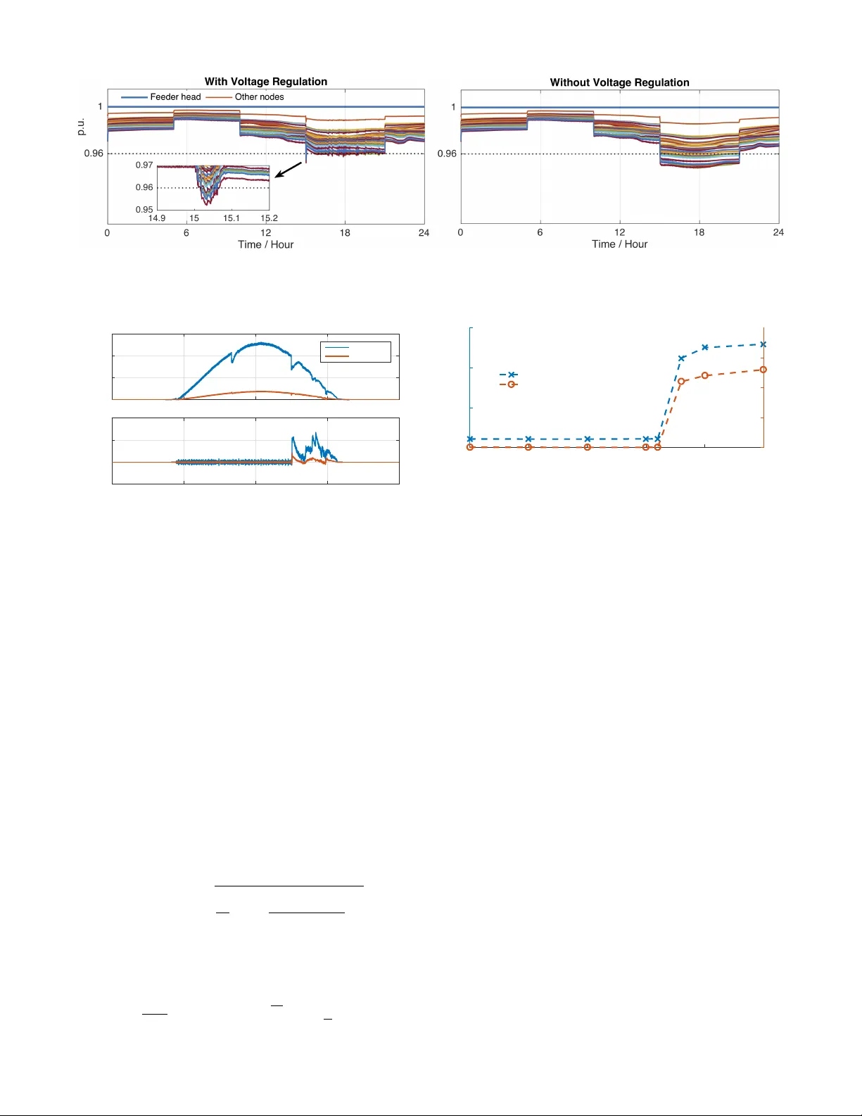
Authors: Yue Chen, Andrey Bernstein, Adithya Devraj
Model-Fr ee Primal-Dual Methods f or Netw ork Optimization with A pplication to Real-T ime Optimal P o wer Flow Y ue Chen 1 , Andrey Bernstein 1 , Adithya De vraj 2 , Sean Meyn 2 Abstract — This paper examines the problem of r eal-time optimization of networked systems and develops online algo- rithms that steer the system towards the optimal trajectory without explicit knowledge of the system model. The pr oblem is modeled as a dynamic optimization problem with time- varying performance objectives and engineering constraints. The design of the algorithms le verages the online zero-order primal-dual projected-gradient method. In particular , the pri- mal step that in volves the gradient of the objective function (and hence requires networked systems model) is replaced by its zero-order approximation with two function ev aluations using a deterministic perturbation signal. The evaluations are performed using the measurements of the system output, hence giving rise to a feedback inter connection, with the optimization algorithm serving as a feedback controller . The paper provides some insights on the stability and tracking properties of this interconnection. Finally , the paper applies this methodology to a real-time optimal power flow pr oblem in power systems, and shows its efficacy on the IEEE 37-node distrib ution test feeder for reference power tracking and voltage regulation. I . I N T RO D U C T I O N This paper considers the problem of real-time optimization of networked systems, where the desired operation of the network is formulated as a dynamic optimization problem with time-varying performance objecti ves and engineering constraints [8], [18], [31]. T o illustrate the idea, consider the following time-varying model that describes the input-output behaviour of the systems in the network: y ( t ) = h t ( x ( t )) (1) where x ( t ) ∈ R n is a vector representing controllable inputs; y ( t ) ∈ R m collects the outputs of the network; and h t ( · ) : R n → R m is a time-varying map representing the system model. Suppose that the desired behaviour of the system is defined via a time-varying optimization problem of the form min x ∈X ( t ) , y = h t ( x ) f t ( y ) (2) where X ( t ) is a con v ex set representing, e.g., engineering constraints; and f t : R m → R is a con ve x function repre- senting the time-v arying performance goals. For simplicity of illustration, we assume that the performance is measured only with respect to the output y . *This work was authored (in part) by the National Renewable Energy Laboratory , operated by Alliance for Sustainable Energy , LLC, for the U.S. Department of Energy (DOE) under Contract No. DE-AC36-08GO28308. 1 Y . Chen and A. Bernstein are with the Power Systems Engineering Center , National Renew able Energy Laboratory , Golden, CO 80401, USA yue.chen@nrel.gov, andrey.bernstein@nrel.gov 2 A. Devraj and S. Me yn are with the Department of Electrical and Computer Engineering, Uni versity of Florida, Gainesville, FL 32611, USA adithyamdevraj@ufl.edu, meyn@ece.ufl.edu In an ideal situation, when infinite computation and communication capabilities are av ailable, one could seek solutions (or stationary points) of (2) at each time t by , e.g., an iterative projected-gradient method: x ( k +1) = Proj X ( t ) n x ( k ) − α ( J ( k ) t ) T ∇ y f t ( h t ( x ( k ) )) o , (3) where k = 0 , 1 , . . . is the iteration index; J ( k ) t := J h t ( x ( k ) ) is the Jacobian matrix of the input-output map h t ; Proj X ( z ) := arg min x ∈X k z − x k 2 denotes projection; and α > 0 is the step size. In practice, this approach might be infeasible. First, running (3) to con vergence might be impossible due to stringent real-time constraints. Second, (3) requires the functional knowledge of the input-output map h t or an approximation thereof in real time. The latter is absent in typical network optimization applications, such as the power distribution system example considered here. T o address the first challenge, we adopt the measurement- based optimization framework of [8], [15], [16], [22], [23], wherein (3) is replaced with a running (or online) version: x ( k +1) = Proj X ( k ) n x ( k ) − α ( J ( k ) ) T ∇ y f ( k ) ( b y ( k ) ) o , (4) in which the iteration inde x k is no w identified with a discrete time instance t k at which the computation is performed; X ( k ) := X ( t k ) , J ( k ) := J h t k ( x ( k ) ) , f ( k ) := f t k ; and b y ( k ) represents the measurement of the network output h t k ( x ( k ) ) at time t k . Note that (4) represents a feedback controller that computes the input to the system based on its output; howe ver , the implementation of this controller requires the real-time model information in the form of J ( k ) . This paper sets out to address the second challenge, and tackle situations in which J ( k ) is not available for real time optimization. This is motiv ated by networked systems optimization problems, such as the optimal po wer flow in power systems considered in Section V, wherein the topol- ogy and parameters of the network, as well as e xogenous inputs, might change rapidly due to variability of working conditions, natural disasters, and cyber-physical attacks. T o address this challenge, we lev erage a zer o-or der approxima- tion of the gradient of the objectiv e function. In particular, we replace the gradient of 1 F ( k ) ( x ) := f ( k ) ( h t k ( x )) ∇ F ( k ) ( x ) = ( J h t k ( x )) T ∇ y f ( k ) ( h t k ( x )) (5) with the two function ev aluation approximation: b ∇ F ( k ) ( x ; ξ , ) := 1 2 ξ h F ( k ) ( x + ξ ) − F ( k ) ( x − ξ ) i (6) 1 A more direct approach is to estimate the Jacobian matrix with a zero- order approximation. This direction is a subject of ongoing research. where ξ ∈ R n is a perturbation (or exploration) vector , and > 0 is a (small) scalar . Observe that this modification requires now measurements of the output at two (rather than one) inputs: x ( k ) ± ξ at each time step k . With this modification, algorithm (4) can be carried out without any knowledge of the map h t . While the stylized algorithm (4) and approximation (6) is used here for an illustration of the main ideas, the paper considers a more general con ve x constrained optimization framew ork, and dev elops model-free primal-dual methods to track the optimal trajectories. Using a deterministic explo- ration approach reminiscent to the quasi-stochastic approx- imation method [5], this paper provides design principles for the exploration signal ξ , as well as other algorithmic parameters, to ensure stability and tracking guarantees. In particular , we show that under some conditions, the iterates x ( k ) con v erge within a ball around the optimal solution of (2). Finally , we apply the de veloped methodology to the problem of distributed real-time v oltage re gulation and po wer setpoint tracking in po wer distribution networks. Much of the analysis is restricted to the case in which the model map h t is linear . Extensions to nonlinear models is a topic of current research. Literatur e Review Zero-order (or gradient-free) optimization has been a subject of interest in the optimization, control, and machine learning communities for decades. The seminal paper of Kiefer and W olfo witz [25] introduced a one-dimensional variant of approximation (6); for a d -dimensional prob- lem, it perturbs each dimension separately and requires 2 d function ev aluations. The simultaneous perturbation stochas- tic approximation (SPSA) algorithm [34] uses zero-mean independent random perturbations, requiring two function ev aluations at each step. In [10], [30], the SPSA algorithm was extended to deterministic perturbations , to impro ve con v ergence rates under the assumption of a vanishing step- size and vanishing quasi-noise . Analysis of the zero-order methods based on two function ev aluation (similar to (6)) has been recently a focus of se veral papers [17], [20], [21], [29]. In these papers, a stochastic exploration signal ξ is used (typically , Gaussian iid) and con v ergence analysis of (projected) gradient methods and various v ariants of the method of multipliers is offered. In the theoretical machine learning community , “bandit optimization” refers to zero-order online optimization algo- rithms based on a single or multiple e v aluations of the objec- tiv e function [3], [13], [19]. These algorithms typically have high variance of the estimate if the ev aluation is performed using one or two function ev aluations [14]. Finally , the gradient-free technique termed “extremum-seeking control” (ESC) [2] le verages sinusoidal perturbation signals and single function ev aluation to estimate the gradient. Stability of the ESC feedback scheme was analyzed in, e.g., [27], [35]. These algorithms typically require additional filters to smooth out the noise introduced by the perturbations. In terms of zero-order network optimization, our work is closely related to the recent work [21], wherein a multi-agent optimization of a class of non-conv ex problems is considered. The paper then develops distributed algorithms based on the zero-order approximation of the method of multipliers. In contrast to our paper , [21] considers a stochastic exploration signal for the gradient estimation, and typically requires N > 2 function ev aluations to reduce the estimation v ariance [21, Lemma 1]; see also [5] for the detailed analysis of the advantage of deterministic vs stochastic exploration. Moreov er , it considers a static optimization problem. Contrary to much of the pre vious work (with the sole exception of perhaps [21]), we consider a constant step- size algorithm, necessitated by our application in a time- varying optimization problem. Moreover , since the problem we consider here is a constrained optimization problem, it leads to the extension of the gradient-free methods to novel model-free primal-dual algorithms. Due to the real-time nature of our application, we resort here to computationally- light online gradient-descent methods rather than variants of methods of multipliers which typically require solving an optimization problem at each time step. Or ganization: The rest of the paper is organized as follows. Section II introduces the general network optimiza- tion problem. Section III proposes the model-free primal- dual algorithm to solve the problem in Section II. The con v ergence of the algorithm is analyzed in Section IV. Section V introduces the po wer systems application and the simulation results are presented in Section VI. Section VII concludes the paper and proposes future works. I I . N E T W O R K O P T I M I Z A T I O N F R A M E W O R K Consider the general network optimization problem [8], wherein at each time step k ∈ N , the goal is to optimize the operation of a network of N systems: min x ∈ R n f ( k ) 0 ( y ( k ) ( x )) + N X i =1 f ( k ) i ( x i ) (7a) sub ject to : x i ∈ X ( k ) i , i = 1 , . . . , N (7b) g ( k ) j ( y ( k ) ( x )) ≤ 0 , j = 1 , . . . , M (7c) where X ( k ) i ⊂ R n i , with P N i =1 n i = n , are con ve x sets representing operational constraints on the control input x i of system i ; and y ( k ) ( x ) is an algebraic representation of some observ able outputs in the netw orked system. In this paper , much of the analysis is restricted to the linear case 2 y ( k ) ( x ) := C x + D w ( k ) ∈ R m (8) where C ∈ R m × n and D ∈ R m × w are giv en model parameters, and w ( k ) ∈ R w is a vector of time-varying exogenous (uncontrollable) inputs. For example, in the po wer systems case considered in Section VI, y ( k ) ( x ) represents the linearized power -flo w equations. 2 Howe ver , the de veloped algorithms, as well as our numerical results in Section VI, are not restricted to the linear case. Further , the con v ex function f ( k ) 0 ( y ( k ) ( x )) : R n → R represent the time-v arying performance goals associated with the outputs y ( k ) ( x ) ; whereas f ( k ) i ( x i ) : R n i → R is a con v ex function representing performance goals of system i . Finally , g ( k ) j ( y ( k ) ( x )) : R m → R are con v ex functions used to impose time-varying constraints on the output y ( k ) ( x ) . Observe that (7) is naturally model-based – in order to solve it, the knowledge of the (linearized) system model (8) and the exogenous input w ( k ) is required. This problem will be used next to define the desir ed operational trajectories for the networked system; in Section III, we propose a model- fr ee algorithm to track these desired operational trajectories. W e define the following shorthand notation: g ( k ) ( y ( k ) ( x )) := h g ( k ) 1 ( y ( k ) ( x )) , . . . , g ( k ) M ( y ( k ) ( x )) i T f ( k ) ( x ) := X i f ( k ) i ( x i ) h ( k ) ( x ) := f ( k ) ( x ) + f ( k ) 0 ( y ( k ) ( x )) . Setting λ ∈ R M + as the vector of dual variables associated with (7c), the Lagrangian function at step k is giv en by: L ( k ) ( x , λ ) := h ( k ) ( x ) + λ T g ( k ) ( y ( k ) ( x )) . (9) Finally , the re gularized Lagrangian function is gi ven by [26]: L ( k ) p,d ( x , λ ) := L ( k ) ( x , λ ) + p 2 k x k 2 2 − d 2 k λ k 2 2 (10) where p > 0 and d > 0 are regularization parameters. W ith this notation at hand, consider the saddle-point problem associated with L ( k ) p,d : max λ ∈D ( k ) min x ∈X ( k ) L ( k ) p,d ( x , λ ) k ∈ N (11) where X ( k ) := X ( k ) 1 × . . . × X ( k ) N and D ( k ) is a conv ex and compact set that contains the optimal dual variable of (11); see, e.g., [8] for details. Hereafter , the optimal trajectory z ( ∗ ,k ) := { x ( ∗ ,k ) , λ ( ∗ ,k ) } k ∈ N of (11) represents the desir ed trajectory . It is clear that L ( k ) p,d ( x , λ ) is strongly conv ex in x and strongly concave in λ ; thus, the optimizer z ( ∗ ,k ) of (11) is unique. Ho wever , z ( ∗ ,k ) might be dif ferent from any saddle point of the exact Lagrangian L ( k ) ( x , λ ) , and the bound on the distance between z ( ∗ ,k ) and the solution of (7) can be established as, e.g., in [26]. T o proceed, we list the assumptions that will be imposed on the different elements of (7). Assumption 1. Slater’ s condition holds at each time step k . Assumption 2. The functions f ( k ) 0 ( y ) and f ( k ) i ( x i ) are con v ex and continuously differentiable. The maps ∇ f ( k ) ( x ) , ∇ f ( k ) 0 ( y ) , and ∇ 2 f ( k ) 0 ( y ) are Lipschitz continuous. Assumption 3. For each j = 1 , . . . , M , the function g ( k ) j ( y ) is con vex and continuously dif ferentiable. Moreo ver , ∇ g ( k ) j ( y ) and ∇ 2 g ( k ) j ( y ) are Lipschitz continuous. Assumption 4. There exists a constant e f such that for all k and x , y : k∇ f ( k ) 0 ( y ) − ∇ f ( k − 1) 0 ( y ) k ≤ e f , k∇ f ( k ) ( x ) − ∇ f ( k − 1) ( x ) k ≤ e f , k∇ g ( k ) j ( y ) − ∇ g ( k − 1) j ( y ) k ≤ e f , j = 1 , . . . , M . I I I . M O D E L - F R E E P R I M A L - D UA L M E T H O D A measurement-based primal-dual method was introduced in [8] to track the desired trajectory { z ( ∗ ,k ) } ; we present the method here for con v enience: x ( k +1) = Proj X ( k ) n (1 − αp ) x ( k ) − α ∇ x f ( k ) ( x ( k ) ) + C T ∇ y f ( k ) 0 ( b y ( k ) ) + M X j =1 λ ( k ) j C T ∇ g ( k ) j ( b y ( k ) ) o (12a) λ ( k +1) = Proj D ( k ) n (1 − αd ) λ ( k ) + α g ( k ) ( b y ( k ) ) o (12b) where α > 0 is a constant step size, and b y ( k ) is a (possibly noisy) measurement of y ( k ) ( x ( k ) ) collected at time step k (see Assumption 5 below). The main advantage of (12) is that it av oids explicit computation of (8) at each time step, and thus does not require kno wledge or estimation of the uncontrollable input w ( k ) appearing in (8). Note that since the method is gradient-based, it relies on the availability of the netw ork model matrix C . Ho we ver , in many practical applications, including the po wer system example of Sec- tion VI, C is time-varying (e.g., due to network topology variation) and its exact value is unav ailable. W e next propose a model-free v ariant of (12). As in the celebrated gradient-free stochastic approximation algorithm of Kiefer and W olfowitz [25], the general idea is to use few (online) ev aluations of the objecti ve function to estimate the gradient. The gradient approximation is justified through a T aylor series expansion as explained next. Let F : R n → R be a C 3 function, whose first and second deriv atives are globally Lipschitz continuous (cf. Assumption 2). For giv en x ∈ R n , this v ariable is perturbed by ± ξ , with ξ ∈ R n and > 0 . According to T aylor’ s theorem, for any x ∈ R n and r ∈ R , F ( x + r ξ ) = F ( x ) + r ξ T ∇ F ( x ) + r 2 2 ξ T ∇ 2 F ( x ) ξ + O ( r 3 ) T aking r = , r = − , and then subtracting yields: F ( x + ξ ) − F ( x − ξ ) = 2 ξ T ∇ F ( x ) + O ( 3 ) (13) This approximation is summarized in Lemma 1 that fol- lows, with the following shorthand notation: b ∇ F ( x ; ξ , ) := 1 2 ξ [ F ( x + ξ ) − F ( x − ξ )] . (14) Lemma 1. Let F : R n → R be a C 3 function, with Lipsc hitz continuous ∇ F and ∇ 2 F . Then, b ∇ F ( x ; ξ , ) = ξξ T ∇ F ( x ) + O ( 2 ) (15) Note that O ( 2 ) = 0 if F is a quadratic function. In applying Lemma 1 to algorithm design, the vector ξ is updated at each iteration of the algorithm. Let { ξ ( k ) } denote a deterministic exploration signal , with ξ ( k ) ∈ R n . It is assumed in this paper that the exploration signal is obtained by sampling the sinusoidal signal ξ i ( t ) = √ 2 sin( ω i t ) , i = 1 , . . . , n, (16) with ω i 6 = ω j for all i 6 = j ; other signals are possible provided that they satisfy Assumption 6 below . The following gradient-free v ariant of the primal-dual algorithm (12) is well motiv ated by Lemma 1. Model-Free Primal-Dual Algorithm At each time step k , perform the follo wing steps: [S1a] (forward exploration) : Apply x ( k ) + := x ( k ) + ξ ( k ) to the system, and collect the measurement b y ( k ) + of the output y ( k ) ( x ( k ) + ) . [S1b] (backward exploration) : Apply x ( k ) − := x ( k ) − ξ ( k ) to the system, and collect the measurement b y ( k ) − of the output y ( k ) ( x ( k ) − ) . [S1c] (control application) : Apply x ( k ) to the system, and collect the measurement b y ( k ) of the output y ( k ) ( x ( k ) ) . [S2a] (approximate gradient) : Compute the approximate gradient for the primal step b ∇L ( k ) := ∇ x f ( k ) ( x ( k ) ) + 1 2 ξ ( k ) h f ( k ) 0 ( b y ( k ) + ) − f ( k ) 0 ( b y ( k ) − ) i + 1 2 ξ ( k ) ( λ ( k ) ) T h g ( k ) ( b y ( k ) + ) − g ( k ) ( b y ( k ) − ) i . (17) [S2b] (approximate primal step) : Compute x ( k +1) = Proj X ( k ) n (1 − αp ) x ( k ) − α b ∇L ( k ) o . (18) [S3] (dual step) : Compute λ ( k +1) = Proj D ( k ) n (1 − αd ) λ ( k ) + α g ( k ) ( b y ( k ) ) o . (19) The following remarks are in order . Remark 1. Lemma 1 alone is not enough to obtain con ver - gence guarantees since the matrix ξξ T is semi-definite b ut not strictly definite. W e formulate conditions for con v ergence in the next section. Remark 2. The algorithm allows distrib uted implementa- tion. This point is illustrated in a power system optimization example described in Section VI. Remark 3. The algorithm requires three measurements of the output: b y ( k ) + , b y ( k ) − , and b y ( k ) . In fact, the third mea- surement can be replaced with, e.g., an average b y ( k ) := 0 . 5( b y ( k ) + + b y ( k ) − ) , provided that b y ( k ) satisfies Assumption 5 below . I V . C O N V E R G E N C E A NA LY S I S For the purpose of the analysis, we assume bounded measurement error . Assumption 5. There exists a scalar e y < ∞ such that the measurement error can be bounded as sup k ≥ 1 k b y ( k ) − y ( k ) ( x ( k ) ) k 2 ≤ e y , sup k ≥ 1 k b y ( k ) + − y ( k ) ( x ( k ) + ) k 2 ≤ e y , sup k ≥ 1 k b y ( k ) − − y ( k ) ( x ( k ) − ) k 2 ≤ e y . The exploration signal plays an important role in the con v ergence of the proposed algorithm. Recall that the exploration signal ξ ( k ) is sampled from a continuous-time signal ξ ( t ) . Recent work on quasi-stochastic approximation [5], [33] and extremum seeking control [1] has shown that certain deterministic exploration signals can help reduce the asymptotic v ariance and improv e con ver gence, in comparison to random exploration (see Fig. 1 of [33]). W e impose the following assumption on the exploration signal. Assumption 6. The exploration signal is a periodic signal with period T , and 1 T Z t + T t ξ ( τ ) ξ ( τ ) T dτ = I (20) for all t , where I is the identity matrix. It can be sho wn that the signal defined in (16) satisfies Assumption 6 with T being a common integer multiple of the sinusoidal signal periods. This strong assumption is imposed to simplify the proofs that follows. It is enough to hav e the approximation: 1 T Z t + T t ξ ( τ ) ξ ( τ ) T dτ = Σ ξ + O (1 /T ) in which Σ ξ is positiv e definite, and the 1 /T bound for the error term is independent of t (this is the assumption used in [5]). An example is the signal defined in (16) in which the frequencies may not have a common multiple. W e first sho w that the primal step (18) is approximately equiv alent to an av eraged primal step, where the singular “gain matrix” ξ ξ T is replaced with the identity matrix (20). This analysis is performed for the algorithm defined in continuous time, which is justified using standard ODE approximation techniques from the stochastic approximation literature [5], [11] or more recent literature on optimization [32], [37]. W e then apply the results of [8] to the resulting approximate primal-dual algorithm to sho w tracking of the desired trajectory { z ( ∗ ,k ) } defined by (11). A. A veraged Primal Step In this section, we provide some preliminary results on the asymptotic properties of the primal iteration (18); a detailed analysis is the subject of ongoing work. T o that end, consider a C 3 strongly con ve x strongly smooth function F and the associated projected gradient descent method: x ( k +1) = Proj X n x ( k ) − α ∇ F ( x ( k ) ) o . (21) The corresponding gradient-free method reads x ( k +1) = Proj X n x ( k ) − α b ∇ F ( x ( k ) ; ξ ( k ) , ) o . (22) Our goal in this section is to explain conditions for con v er- gence of (22). W e cannot expect con vergence of { x ( k ) } to a limit as k → ∞ . W e might expect something like the ergodic steady-state obtained for stochastic approximation with fixed stepsize [11]. In this section, we are content to simply obtain bounds on the error k x ( k ) − x ∗ k , where x ∗ is the minimizer of F . Under appropriate assumptions, for a continuous time model we obtain lim sup t →∞ k x ( t ) − x ∗ k = O ( α + 2 ) (23) See Remark 4 at the close of this section. According to Lemma 1, the continuous-time analogue of (22) is giv en by ˙ x ( t ) = Proj T X ( x ( t )) { α β ( t, x ( t )) } (24) where, T X ( x ) is the cone of tangent directions of X at x (or for short, the tangent cone of X at x ), and for any t and x , β ( t, x ) := − ξ ( t ) ξ ( t ) T ∇ F ( x ) + O ( 2 ) . (25) The function β is Lipschitz continuous in x , uniformly in t . Analysis of the continuous projection in (24) is a topic of research. W e consider here a simplification in which the projection is only applied at integer multiples of the period T . At stage K + 1 of the algorithm, we hav e computed x ( K T ) , and with this initial condition, { x ( t ) : K T ≤ t < ( K + 1) T } is defined as the solution to the ODE without projection: ˙ x ( t ) = α β ( t, x ( t )) (26) W e then define x (( K + 1) T ) = Proj K n x ( K T ) + α Z ( K +1) T K T β ( τ , x ( τ )) dτ o (27) where the projection is onto the set of states corresponding to constraints on x ( K T ) . This recursion admits an approximation by a projected gradient descent algorithm: Lemma 2. Suppose F is C 3 , and that both ∇ F and ∇ 2 F ar e globally Lipschitz continuous. Suppose mor eover that Assumption 6 holds. Then, the solutions to (26) admit the appr oximation: x (( K + 1) T ) = Proj K { x − αT ( ∇ F ( x ) + s K ( x )) } (28) wher e x = x ( K T ) , and s K ( x ) = O ( α + 2 ) . Pr oof. It is enough to approximate the integral appearing in (27). Under the Lipschitz conditions and boundedness of ξ , there exists a constant b 0 < ∞ such that for all K T ≤ τ < ( K + 1) T , k x ( τ ) − x ( K T ) k ≤ b 0 T α, k β ( τ , x ( τ )) − β ( τ , x ( K T )) k ≤ b 0 T α. Consequently , for τ in this range, β ( τ , x ( τ )) = β ( τ , x ( K T )) + O ( α ) = − ξ ( τ ) ξ ( τ ) T ∇ F ( x ( K T )) + O ( 2 ) + O ( α ) Under Assumption 6, it follows that Z ( K +1) T K T β ( τ , x ( τ )) dτ = − T ∇ F ( x ( K T )) + O ( α + 2 ) , which completes the proof. Remark 4. If k∇ F k is coercive, then techniques used to establish stability of gradient descent can be used to show that the solution to (26) is ultimately bounded [28]. If F is L -smooth and µ -strongly conv ex then we obtain the uniform bound (23), independent of the initial condition. B. T racking of the Desir ed T rajectory W e note that Lemma 2 suggests that the primal iteration (18) can be viewed as an approximate projected gradient descent iteration on the primal variable provided that: (i) α and are chosen small enough, and (ii) the projection is performed periodically , ev ery T time instances. In that case, iteration (18)-(19) is equi valent to: x ( k +1) = Proj k n x ( k ) − α ∇ x L ( k ) p,d ( z ( k ) ) + O ( α + 2 + e f + e y ) o (29a) λ ( k +1) = Proj D ( k ) n (1 − αd ) λ ( k ) + α g ( k ) ( b y ( k ) ) o , (29b) where where z ( k ) := { x ( k ) , λ ( k ) } , and Proj k is the projec- tion onto X ( k ) for k a multiple of T / ∆ t ( ∆ t is the time discretization step). W e note that the additional term O ( e y ) in (29) is due to the use of measurements in (18) instead of the exact system output (cf. Assumption 5). Finally , the additional term O ( e f ) is due to the time-variability of the Lagrangian ov er the period of T time instances as quantified by Assumption 4. W e next analyze the tracking properties of (29). T o this end, quantify the temporal v ariability of the desired trajectory z ( ∗ ,k ) via σ ( k ) := k z ( ∗ ,k +1) − z ( ∗ ,k ) k 2 . (30) In addition, let φ ( k ) : z 7→ " ∇ x L ( k ) p,d ( z ) − g ( k ) ( y ( k ) ( x )) + d λ # (31) denote the primal-dual operator associated with (11). The following holds (see, e.g., [8, Lemma 5]). Lemma 3. Ther e exist constants 0 < η φ ≤ L φ < ∞ such that, for every k ∈ N , the map φ ( k ) ( z ) is strongly monotone over X ( k ) × D ( k ) with constant η φ and Lipschitz over X ( k ) × D ( k ) with coefficient L φ . Finally , let b φ ( k ) : z 7→ " ∇ x L ( k ) p,d ( z ) + O ( α + 2 + e f + e y ) − g ( k ) ( b y ( k ) ) + d λ # , (32) denote the approximate primal-dual operator associated with (29). Using [8, Lemma 4], the follo wing result follows. Lemma 4. Ther e exists a constant φ = O ( α + 2 + e f + e y ) such that φ ( k ) ( z ( k ) ) − b φ ( k ) ( z ( k ) ) 2 ≤ φ , ∀ k = 1 , 2 , . . . (33) W e use [8, Theorem 4] to sho w that the approximate time-varying primal-dual algorithm (18)–(19) e xhibits the following tracking performance. Theorem 1. Suppose that the step size α is chosen such that 0 < α < 2 η φ /L 2 φ . Mor eover , suppose that ther e e xists a scalar σ < ∞ such that sup k ≥ 1 σ ( k ) ≤ σ . Then, the sequence { z ( k ) } con ver ges Q-linearly to { z ( ∗ ,k ) } up to an asymptotic err or bound given by: lim sup k →∞ k z ( k ) − z ( ∗ ,k ) k 2 ≤ α φ + σ 1 − c (34) wher e c := q 1 − 2 αη φ + α 2 L 2 φ < 1 and φ = O ( α + 2 + e f + e y ) . V . M O D E L - F R E E R E A L - T I M E O P T I M A L P OW E R F L O W The application considered in this paper is real-time optimization of the power injections of distributed ener gy resources (DERs) in a distribution system. The following objectiv es are pursued: (i) feeder head/substation power is following a prescribed signal, and (ii) the voltages are regulated within prescribed bounds. This is achiev ed via formulating an optimal po wer flow (OPF) problem of the form (7) and seeking its solutions in real time using the model-free primal-dual frame work introduced in Section III. Consider a distrib ution system that is described by a set of nodes N = { 0 , . . . , n } , where node 0 denotes the feeder head (or substation) with fixed voltage; the rest are P Q nodes. In this work, we focus on controlling the batteries and PV systems in the distribution system interfaced via power in v erters; howe ver , the proposed framew ork can be easily extended to include other types of DERs. Let N bt and N pv be the number of batteries and PVs, respectively . So the total number of DERs N der = N bt + N pv . A. Notation For notation bre vity , in this section, we drop the algorithm iteration superscript ( k ) from v ariable names, unless other- wise specified. The distribution system is described by the A C power -flo w equations, defining input-output relationship of this physical system. In particular: • x ∈ R 2 N der collects all decision variables, where each DER has real and reactive po wer x i = { x i,p , x i,q } ; • ` ∈ R 2 n collects the activ e and reactiv e power of uncontrollable loads (the “noise”); • v ( x , ` ) ∈ R n collects the voltage magnitudes at ev ery P Q node; and • P 0 ( x , ` ) ∈ R is the power flow at the feeder head. The (non-linear) maps ( v ( x , ` ) , P 0 ( x , ` )) exists under some conditions and are defined by the power -flo w equations [9]. The goal is to control the output ( v ( x , ` ) , P 0 ( x , ` )) by controlling x . In order to formulate a con ve x target OPF (7), an approxi- mate linearized relationship between the output y := ( v , P 0 ) and the input ( x , ` ) is lev eraged. In particular , at each time step k , the output is approximated as y = C x + D ` + y 0 ; (35) see, e.g., [9]. W e would like to emphasize that the relation- ship (35) is used only to define the desired trajectory via (7) and (11); the actual simulation belo w is performed using the exact (nonlinear) power-flo w equations. B. Objective Function The objective function (7a) consists of two parts: f 0 ( x ) =( P 0 ( x , ` ) − P • 0 ) 2 (36a) f i ( x i ) = c i,p x 2 i,p + c i,q x 2 i,q + c i,p • ( x i,p − x • i,p ) 2 (36b) where c i,p , c i,q , and c i,p • are weighting parameters for the DER i . The global cost (36a) dri ves the substation real po wer P 0 to follow the reference po wer P • 0 , which is usually time- varying. The local DER cost (36b) penalizes the control effort and the difference between the control and its desired reference power . F or a PV system, the reference power x • i,p is the real-time maximal PV power generation; for a battery system, the reference x • i,p is the power to reach the preferred state of charge (SOC), which is usually set as the middle point of SOC to allow maximal operation flexibility . C. Constraints Constraints associated with the OPF are summarized be- low . 1) V oltage: Each node needs to maintain a stable voltage magnitude within a certain range. For any node i ∈ N , V i ≤ v i ( x , ` ) ≤ V i (37) 2) Battery: Battery limits are imposed on battery control variables to enable feasible operations. Each battery has its power and energy limits: X i,p ≤ x i,p ≤ X i,p , S O C i ≤ S OC i ≤ S OC i where S O C i represents the SOC of battery i . Consider the battery charging/dischar ging dynamics S O C ( k +1) i = S O C ( k ) i + x ( k ) i,p ∆ t, where ∆ t is the time step in one iteration. The energy limit can be rewritten as power constraints S O C i − S O C ( k +1) i ∆ t ≤ x ( k ) i,p ≤ S O C i − S O C ( k +1) i ∆ t Letting X bt i = max X i,p , S O C i − S O C ( k +1) i ∆ t ! X bt i = min X bt i,p , S O C i − S O C ( k +1) i ∆ t ! we obtain following constraints for battery i : X bt i ≤ x i,p ≤ X bt i , x 2 i,p + x 2 i,q ≤ ( S bt i ) 2 (40) where S bt i is the upper bound of battery apparent power . 3) PV : Driv en by time-varying solar radiation, PV sys- tems ha ve time-varying limits. Let P pv i and S pv i denote the av ailable activ ate power and apparent power , respectiv ely . The following constraints are imposed on PV i : 0 ≤ x i,p ≤ P pv i , x 2 i,p + x 2 i,q ≤ ( S pv i ) 2 (41) D. Distributed Algorithm Implementation The OPF associated with cost function (36) and constraints (37), (40), (41) can be reformulated as a saddle-point prob- lem of the form of (11), which can then be solved using the model-free primal-dual algorithm proposed in Section III. In fact, the Lagrangian (10) can be decomposed with respect to each DER. The cost function (36b) and constraints (40), (41) are concerned with only local DER informa- tion. They hav e an explicit form of gradient with respect to each local DER control/dual variables. In addition, the measurement-based global information f 0 ( b y + ) and f 0 ( b y − ) that is associated with (36a), as well as the constraint function g ( b y ) that is associated with (37), can be broad- cast to each DER in real time. Therefore, each DER has necessary information to locally update its control and dual variables. This gather-and-broadcast control architecture was previously considered in, e.g., [7], [16], in the model-based context. One practical concern in the distributed implementation is the asynchronicity in the control signals and measurements. At each time step, it is possible that DERs do not implement their control signals at the same time, and the measurements might not capture the system response after all local control implementations. It is particularly true for fast communica- tion and control. In fact, the asynchronicity can be modeled as an additional noise source, and can be analyzed similarly to, e.g., [6]. In the next section, we numerically ev aluate the sensitivity of our approach to different lev els of noise. V I . N U M E R I C A L S T U DY A. Simulation Setup Numerical experiments were conducted on a modified IEEE 37-node test feeder to demonstrate the proposed model- free OPF . W e used a single-phase v ariant of the original test 79 9 70 1 74 2 70 5 70 2 72 0 70 4 71 3 70 7 72 2 70 3 74 4 72 9 72 8 72 7 70 6 72 5 71 8 71 4 73 0 73 1 70 9 70 8 73 2 77 5 73 3 73 6 73 4 71 0 73 5 73 7 73 8 71 1 74 1 74 0 72 4 71 2 Fig. 1. Modified IEEE 37-node test feeder: PV and battery nodes are labeled by circles and squares, respectively . T ABLE I C O NFI G U R A T I O N O F D E R S Node PV Capacity (kV A) Battery Capacity SOC (MWh) Active P ower (MW) Appar ent Po wer (MV A) 703 N/A [0 30] [ − 10 10] 12 709 200 N/A 711 200 N/A 712 200 N/A 713 100 N/A 724 100 N/A 730 200 N/A 734 200 [0 30] [ − 10 10] 12 740 200 N/A feeder [24], with DERs connected at dif ferent locations. Fig. 1 shows the feeder diagram. T able I provides the configu- ration for these DERs, and the efficienc y of the batteries is assumed to be 0.9. In simulation, the load and PV data were obtained from the real data in California [4]. They were smoothed and scaled to an appropriate magnitude for the considered distrib ution system. The total demand and available PV generation in a typical day are gi ven in Fig. 2. The described distrib ution system w as simulated using Matpower [38], from where the feeder head activ e po wer and node voltages are obtained as system outputs. The output measurements were obtained by adding Gaussian noises to the simulated outputs; in particular, b y ( k ) i = y ( k ) i + W y ( k ) i (42) where the random v ariable W follows the normal distribution N (0 , σ 2 ) . In simulations, unless otherwise stated, σ = 0 . 001 , which is consistent with the standard phasor measurement units noise values [12], [36]. T ABLE II A L GO R I T HM PA RA M E TE R S U S E D I N T H E S I M UL A T I ON . Coefficients in the cost function (36b) c pv i,p c pv i,q c pv i,p • c bt i,p c bt i,p c bt i,p • V alue 1 × 10 − 5 1 × 10 − 5 1 × 10 − 3 1 / 6 × 10 − 4 1 / 6 × 10 − 4 1 / 6 × 10 − 4 Step sizes (control variables) α pv i,p a pv i,q a bt i,p a bt i,q V alue 2 2 12 12 Step sizes (dual variables) α ¯ v α v α pv i, ¯ P α pv i,P α pv i, ¯ S α bt i, ¯ P α bt i,P α bt i, ¯ S V alue 10 10 1 × 10 − 3 1 × 10 − 3 1 × 10 − 3 2 × 10 − 4 2 × 10 − 4 1 × 10 − 3 0 6 12 18 24 0 20 40 60 80 MW Toal loads 0 6 12 18 24 Time / Hour 0 5 10 15 MW Available PV power Total Node 705 Fig. 2. T otal load and available PV generation in one day , and an example of a vailable PV generation at one node. Algorithm parameters were configured as shown in T able II. For each local controller, the sine signal was chosen as the perturbation signal: ξ n ( t ) = √ 2 sin (2 π f n t ) , t ∈ [0 24 hr ] where the time step ∆ t = 1 second; = 0 . 001 √ 2 S base , with base power S base = 23 . 04 MV A; and the frequency f n was uniquely chosen from the range [1 / 7 . 1 , 1 / 26] Hz. B. Simulation Results The results described here are based on the 24-hour simulation with the load and PV data given in Fig. 2. It is observed from Fig. 3 that the feeder head power nicely tracks the desired reference power and the DERs can respond quickly to unforeseen changes of the reference signal. The subplots on the bottom of Fig. 3 show the detailed response when the reference signal was changed. The power tracking is less accurate during [15 , 21] hours, because the po wer tracking was conflicting with another objective of v oltage regulation. The performance of voltage regulation is illustrated in Fig. 5, which provides the comparison of node v oltages with and without voltage regulation. The voltage lower limit was set to 0.96 p.u. At the time around 15 hours, when some node voltages dropped belo w the limit, they were recovered quickly to normal values. In contrast, without regulation (no voltage limit), some node v oltages stayed below 0.96 p.u. for the next 6 hours. 0 6 12 18 24 Time / Hour 0 20 40 60 MW Feeder head Reference 5 5.1 0 10 20 30 10 10.1 0 10 20 30 15 15.1 20 30 40 50 21 21.1 20 30 40 50 Fig. 3. Performance of feeder head po wer tracking achie ved by the gradient-free approach. These grid services were provided through the control of battery and PV systems, whose behaviors are presented in Fig. 4 and Fig. 6, respectiv ely . The feeder head po wer was controlled using the active power of DERs, mainly -10 0 10 MW Real power Battery 1 Battery 2 -10 0 10 Mvar Reactive power 0 5 10 MVA Apparent power 0 6 12 18 24 Time / Hour 0 10 20 30 MWh SOC Fig. 4. Control results of tw o battery systems. The dashed lines represent hard physical constraints imposed on batteries. Corresponding to each hard constraint, the soft constraint is slightly more conservati ve than the hard constraint, shown as the dotted lines. Soft constraints enable smooth transition of control signals to avoid hard-constraint projections. Fig. 5. Improv ement of voltage profile by the proposed model-free OPF algorithm. 0 5 10 15 MW Real power Aggregate Node 705 0 6 12 18 24 Time / Hour -2 0 2 4 Mvar Reactive power Fig. 6. Results of PV power control. from batteries. The PV systems hav e its main objectiv e of curtailment minimization, so the acti ve PV po wer was merely increased because it is already near the maximal generation. But the active PV power can be largely curtailed when the system requested less power generation (e.g., at time 10, 15 hours). Because the active power of DERs is determined to track the reference feeder head power , the voltage re gulation is mainly accomplished by the reactiv e power of DERs. At the time around 15 hours when some node voltages dropped below the lower limit, the reactiv e po wer from both batteries and PVs acted quickly to reco ver these v oltages to the normal range. T o study the impact of the measurement noise, we tested the proposed algorithm with dif ferent lev els of noise, dis- tinguished by the standard deviation of the noise signal in (42). T wo metrics are used to quantify system performance. The normalized root mean squared error (NRMSE) is used to define power tracking performance: NRMSE = v u u t 1 K K X k =1 P ( k ) 0 − P • ( k ) 0 P • ( k ) 0 ! 2 The a verage v oltage violation (A VV) is used to define voltage regulation performance: A VV = 1 N K N X i =1 K X k =1 [ v ( k ) i − V i ] + + [ V i − v ( k ) i ] + 0 0.5 1 1.5 2 2.5 Standard deviation of noise, σ × 10 -3 0 0.1 0.2 0.3 0.3 NRMSE 0 0.5 1 1.5 AVV ( × 10 -3 p.u.) Power tracking error Voltage violation Fig. 7. The performance is impacted by the measurement noise. where N and K are the number of nodes and simulation time steps, respecti vely; the operator [ ] + projects a neg ativ e value to zero. Fig. 7 shows simulation results of NRMSE and A VV . As the noise signal increases and crosses the point of σ = 1 . 6 × 10 − 3 , the control performance degrades significantly . It is because large measurement noise can suppress the ex- ploration output and leads to inaccurate gradient estimation. One idea to address this issue is to increase the exploration signal to a reasonable magnitude. But the improvement space is limited because of practical system considerations. In that case, we can apply state estimation techniques to filter out measurement noises. It is beyond the scope of this paper and left to our future work. V I I . C O N C L U S I O N S A N D F U T U R E W O R K In this paper , we dev eloped a model-free primal-dual method to track desired trajectories of networked systems. The algorithm leverages the zero-order deterministic esti- mation of the gradient with two function ev aluations. W e provided preliminary stability and tracking results, and il- lustrated an application of the method to real-time OPF in power systems. Analysis of the exact iteration (18)-(19), with the projec- tion performed at every time step, remains an interesting research topic. The promising direction here is to analyze the time-v arying projected dynamics of the form (24). Also, analysis of the asynchronous model-free algorithm is impor- tant from the practical perspectiv e. Finally , on the application side, it would be interesting to show the performance of the algorithm on a more dynamic scenario, including topology reconfigurations (e.g., due to natural disasters and attacks on the grid). R E F E R E N C E S [1] K. Ariyur and M. Krstic. Real-T ime Optimization by Extremum- Seeking Contr ol . Wiley-interscience publication. W iley , 2003. [2] K. B. Ariyur and M. Krsti ´ c. Real T ime Optimization by Extr emum Seeking Contr ol . John Wile y & Sons, Inc., New Y ork, NY , 2003. [3] B. A werbuch and R. Kleinberg. Online linear optimization and adaptiv e routing. Journal of Computer and System Sciences , 74(1):97 – 114, 2008. Learning Theory 2004. [4] J. Bank and J. Hambrick. Dev elopment of a high resolution, real time, distribution-lev el metering system and associated visualization, modeling, and data analysis functions. May 2013. [5] A. Bernstein, Y . Chen, M. Colombino, E. Dall’Anese, P . Mehta, and S. Meyn. Optimal rate of conver gence for quasi-stochastic approximation. T o appear , IEEE CDC and arXiv:1903.07228 , Mar 2019. [6] A. Bernstein and E. Dall’Anese. Asynchronous and distributed tracking of time-v arying fixed points. In 2018 IEEE Conference on Decision and Control (CDC) , pages 3236–3243, Dec 2018. [7] A. Bernstein and E. Dall’Anese. Real-time feedback-based optimiza- tion of distribution grids: A unified approach. IEEE T ransactions on Contr ol of Network Systems , 6(3):1197–1209, Sep. 2019. [8] A. Bernstein, E. Dall’Anese, and A. Simonetto. Online primal- dual methods with measurement feedback for time-v arying conv ex optimization. IEEE T ransactions on Signal Processing , 67(8):1978– 1991, April 2019. [9] A. Bernstein, C. W ang, E. Dall’Anese, J. Le Boudec, and C. Zhao. Load flow in multiphase distribution networks: Existence, uniqueness, non-singularity and linear models. IEEE T ransactions on P ower Systems , 33(6):5832–5843, Nov 2018. [10] S. Bhatnagar , M. C. Fu, S. I. Marcus, and I.-J. W ang. T wo- timescale simultaneous perturbation stochastic approximation using deterministic perturbation sequences. ACM T rans. Model. Comput. Simul. , 13(2):180–209, 2003. [11] V . S. Borkar . Stoc hastic Appr oximation: A Dynamical Systems V iewpoint . Hindustan Book Agency and Cambridge Univ ersity Press (jointly), Delhi, India and Cambridge, UK, 2008. [12] M. Brown, M. Biswal, S. Brahma, S. J. Ranade, and H. Cao. Characterizing and quantifying noise in pmu data. In 2016 IEEE P ower and Energy Society General Meeting (PESGM) , pages 1–5, July 2016. [13] S. Bubeck and N. Cesa-Bianchi. Regret analysis of stochastic and non- stochastic multi-armed bandit problems. F oundations and T r ends R in Machine Learning , 5(1):1–122, 2012. [14] T . Chen and G. B. Giannakis. Bandit conve x optimization for scalable and dynamic iot management. IEEE Internet of Things Journal , 6(1):1276–1286, Feb 2019. [15] M. Colombino, E. Dall’Anese, and A. Bernstein. Online optimization as a feedback controller: Stability and tracking. IEEE T ransactions on Contr ol of Network Systems , pages 1–1, 2019. [16] E. Dall’Anese and A. Simonetto. Optimal po wer flo w pursuit. IEEE T ransactions on Smart Grid , 9(2):942–952, March 2018. [17] J. C. Duchi, M. I. Jordan, M. J. W ainwright, and A. Wibisono. Optimal rates for zero-order conv ex optimization: The po wer of two function ev aluations. IEEE T ransactions on Information Theory , 61(5):2788– 2806, May 2015. [18] M. Fazlyab, C. Nowzari, G. J. Pappas, A. Ribeiro, and V . M. Preciado. Self-T riggered Time-V arying Conv ex Optimization. In Pr oceedings of the 55th IEEE Conference on Decision and Control , pages 3090 – 3097, Las V egas, NV , US, December 2016. [19] A. D. Flaxman, A. T . Kalai, and H. B. McMahan. Online con vex optimization in the bandit setting: Gradient descent without a gradient. In Proceedings of the Sixteenth Annual ACM-SIAM Symposium on Discr ete Algorithms , SOD A ’05, pages 385–394, Philadelphia, P A, USA, 2005. Society for Industrial and Applied Mathematics. [20] X. Gao, B. Jiang, and S. Zhang. On the information-adaptive variants of the admm: An iteration comple xity perspecti ve. Journal of Scientific Computing , 76(1):327–363, Jul 2018. [21] D. Hajinezhad, M. Hong, and A. Garcia. Zone: Zeroth order noncon- vex multi-agent optimization over networks. IEEE T ransactions on Automatic Control , pages 1–1, 2019. [22] A. Hauswirth, S. Bolognani, G. Hug, and F . D ¨ orfler. Projected gradient descent on riemannian manifolds with applications to online power system optimization. In 2016 54th Annual Allerton Confer ence on Communication, Control, and Computing (Allerton) , pages 225–232, Sep. 2016. [23] A. Hauswirth, I. Suboti ´ c, S. Bolognani, G. Hug, and F . D ¨ orfler. T ime- varying projected dynamical systems with applications to feedback optimization of power systems. In 2018 IEEE Conference on Decision and Contr ol (CDC) , pages 3258–3263, Dec 2018. [24] W . H. Kersting. Distribution system modeling and analysis . CRC press, 2006. [25] J. Kiefer and J. W olfowitz. Stochastic estimation of the maximum of a re gression function. Ann. Math. Statist. , 23(3):462–466, 09 1952. [26] J. Koshal, A. Nedi ´ c, and U. Y . Shanbhag. Multiuser optimization: Distributed algorithms and error analysis. SIAM J. on Optimization , 21(3):1046–1081, 2011. [27] M. Krsti ´ c and H.-H. W ang. Stability of extremum seeking feedback for general nonlinear dynamic systems. Automatica , 36(4):595 – 601, 2000. [28] Y . Nesterov . Intr oductory Lectur es on Conve x Optimization: A Basic Course . Springer , 1 edition, 2014. [29] Y . Nesterov and V . Spokoiny . Random gradient-free minimization of con ve x functions. F oundations of Computational Mathematics , 17(2):527–566, Apr 2017. [30] L. Prashanth, S. Bhatnagar , N. Bhavsar, M. C. Fu, and S. Marcus. Random directions stochastic approximation with deterministic per- turbations. IEEE T ransactions on Automatic Contr ol , 2019. [31] S. Rahili and W . Ren. Distributed continuous-time conv ex optimization with time-varying cost functions. IEEE T ransactions on Automatic Contr ol , 62(4):1590–1605, April 2017. [32] B. Shi, S. S. Du, W . J. Su, and M. I. Jordan. Acceleration via Symplectic Discretization of High-Resolution Differential Equations. arXiv e-prints , page arXiv:1902.03694, Feb 2019. [33] D. Shirodkar and S. Meyn. Quasi stochastic approximation. In Pr oceedings of the 2011 American Control Conference , pages 2429– 2435, June 2011. [34] J. C. Spall. Multivariate stochastic approximation using a simultaneous perturbation gradient approximation. IEEE Tr ansactions on Automatic Contr ol , 37(3):332–341, March 1992. [35] H.-H. W ang and M. Krsti ´ c. Extremum seeking for limit cycle minimization. IEEE T ransactions on Automatic Contr ol , 45(12):2432– 2436, Dec 2000. [36] L. Xie, Y . Chen, and P . R. Kumar . Dimensionality reduction of synchrophasor data for early event detection: Linearized analysis. IEEE T ransactions on P ower Systems , 29(6):2784–2794, Nov 2014. [37] J. Zhang, A. Mokhtari, S. Sra, and A. Jadbabaie. Direct runge-kutta discretization achiev es acceleration. In Proceedings of the Interna- tional Conference on Neural Information Pr ocessing Systems (and arXiv:1805.00521) , pages 3904–3913, USA, 2018. Curran Associates Inc. [38] R. D. Zimmerman, C. E. Murillo-Sanchez, and R. J. Thomas. Mat- power: Steady-state operations, planning, and analysis tools for power systems research and education. IEEE T ransactions on P ower Systems , 26(1):12–19, Feb 2011.
Original Paper
Loading high-quality paper...
Comments & Academic Discussion
Loading comments...
Leave a Comment