Function Preserving Projection for Scalable Exploration of High-Dimensional Data

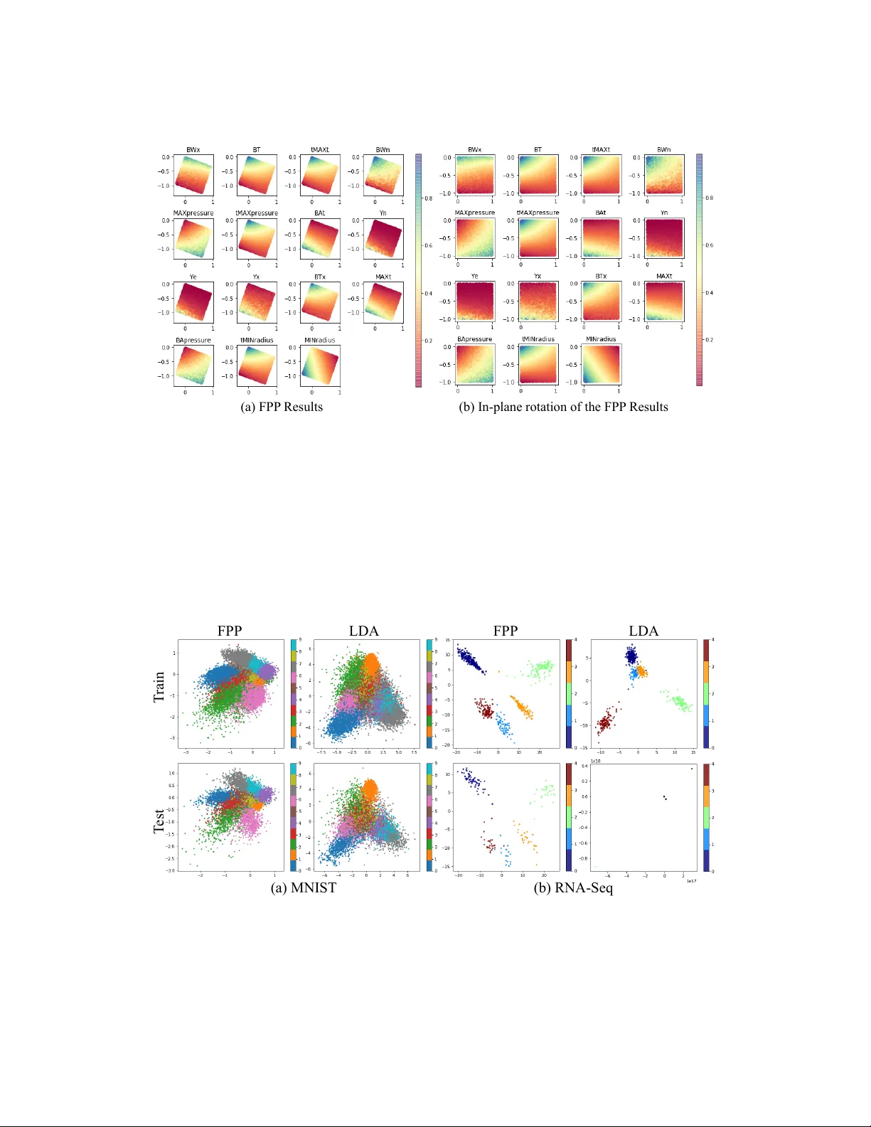
Function Pr eserving Pr ojection f or Scalable Exploration of High-Dimensional Data Shusen Liu, Rushil Anirudh, Jayaraman J . Thiagarajan and Peer -Timo Br emer Lawrence Li vermore National Laboratory 7000 East A v e, Liv ermore, CA 94550 {liu42, anirudh1, jayaraman1, bremer5}@llnl.gov Abstract W e present function pr eserving pr ojections (FPP), a scalable linear projection technique for discovering interpretable relationships in high-dimensional data. Con ventional dimension reduction methods aim to maximally preserve the global and/or local geometric structure of a dataset. Howe ver , in practice one is often more interested in determining ho w one or multiple user -selected r esponse func- tion(s) can be explained by the data. T o intuitiv ely connect the responses to the data, FPP constructs 2D linear embeddings optimized to re veal interpretable yet potentially non-linear patterns of the response functions. More specifically , FPP is designed to (i) produce human-interpretable embeddings; (ii) capture non-linear relationships; (iii) allo w the simultaneous use of multiple response functions; and (iv) scale to millions of samples. Using FPP on real-world datasets, one can obtain fundamentally ne w insights about high-dimensional relationships in lar ge-scale data that could not be achiev ed using existing dimension reduction methods. 1 Introduction The rapid advances in both e xperimental and computational capabilities have resulted in a deluge of data being collected in all branches of science and engineering. Whether this data describes outputs of computer simulations or observ ations from experiments, it is imperati ve to uncov er patterns and relationships in the resulting high-dimensional data to gain insights into the underlying phenomena. Existing solutions for high dimensional analysis struggle to balance the comple xity of an approach with the need to interpret the results. For example, one may fit a linear model which is easily understood yet cannot recov er non-linear patterns or deploy more general techniques, such as deep neural networks, which are more flexible but dif ficult to interpret. Similarly , simple visual encodings such as scatterplot matrices and parallel coordinates Inselber g and Dimsdale [1990], Carr et al. [1987] are easy to read but do not scale to large dimensions. Non-linear dimension reduction can sometimes address the dimensionality challenge at the cost of losing interpretability as axes lose their meaning. Furthermore, man y existing visualization techniques for high-dimensional data do not scale gracefully to large datasets. Instead, we need an approach that can deal with large data and non-linear relationships while remaining interpretable. Function preserving projections (FPP) achiev e both objecti ves by focusing on specific aspects of data through the lens of user-selected r esponse functions. Response function(s) typically correspond to one or multiple diagnostic measurements or simulation outputs, defined at each data point, and can provide a po werful window into underlying patterns in the data. More specifically , rather than aiming to preserve the entire neighborhood structure of high-dimensional data in hopes of finding interesting patterns, we deliberately search for the best linear projection, such that the chosen response functions create an interpretable pattern in the projected space. An important consequence of focusing on the projected response function is that FPP inherently ignores Preprint domain variables and structures not pertinent to the response and does not require the domain to hav e a low intrinsic dimension. The latter is a key property in many applications, most notably simulation ensembles, where the domain is defined as a uniform sampling of a high dimensional hypercube. In these cases, dimension reduction is futile as – by definition – there exists no low dimensional structure in the domain one could discov er and thus many of the traditional techniques do not apply . W e consider a pattern interpretable if it can be approximated by a chosen re gressor and by adjusting the type and order of the regressor , i.e., polynomial vs. e xponential, linear vs. non-linear , etc., we allo w users to choose the complexity of the pattern they deem acceptable. The key insight dri ving the de velopment of FPP is the fact that interpreting non-linear embeddings is challenging yet humans are highly skilled in understanding non-linear patterns. By restricting the initial project to a linear map FPP preserves the interpretability of the resulting plots, i.e., axis labels, while non-linear re gressors enable us to discov er noisy and non-linear relationships. Conceptually , FPP is a dual approach to kernel machines in machine learning, which employ non- linear , and often infinite-dimensional mappings to enable the use of simple linear models for complex data. From a visual e xploration standpoint, we argue that the use of linear models in 2 D is not necessary since humans can still interpret more complex relationships. On the other hand, non-linear mappings of the data coordinates are not e xplainable, thereby making the subsequent analysis also highly opaque. Another crucial feature of FPP is that it supports much larger data than related techniques and enables unified analysis with multiple response functions, wherein a single 2 D projection is identified that jointly preserves all responses. Finally , an often-ov erlooked challenge for view-finding or an y pattern detection algorithm is that, in higher dimensions, it is challenging to qualitativ ely distinguish between meaningful structure and artifacts. This beha vior can be directly attributed to the curse of dimensionality , where the sample sizes used are not suf ficient to make meaningful inferences about the data. In the case of view-finding approaches like FPP , this manifests as ov erfitting, where one can almost al ways create a seemingly meaningful pattern given lo w enough sample counts and sufficiently high dimensions. T o address this problem we argument the 2 D embeddings with the equiv alent of a p -statistic that quantifies the likelihood of the gi ven hypothesis (the observed pattern) to occur in a random function. This, for the first time, provides a quantitati ve and easy to interpret indicator on ho w reliable a gi ven visualization is likely to be, which is crucial to confidently infer new insights. Using sev eral case studies we sho w that FPP pro vides comprehensiv e insights that cannot be easily obtained using con ventional techniques. 2 Related W ork Even though FPP produces linear projections, it is fundamentally different from existing linear dimension reduction techniques like principal component analysis (PCA) Jolliffe [2011]. Dimension reduction, as currently understood, is typically aimed at preserving global (PCA) or local neigh- borhood structures (locality preserving projection He and Niyogi [2004]) of the high-dimensional point geometry . The resulting projection is then colored according to a response function in hopes of highlighting interesting relationships. Howe ver , when analyzing particular response functions the complete geometry of the point set may not be rele vant and can e ven be detrimental by introducing “spurious” variations unrelated to the response of interest. Instead, FPP directly targets the response functions of interest and preserves only the aspects of the high dimensional geometry relev ant to the problem. In this context, FPP is similar to cross decomposition approaches, such as canonical component analysis (CCA) Hardoon et al. [2004] and partial least square (PLS) Chin et al. [1998]. CCA aims to find the subspace that best aligns the domain and the range of a high-dimensional function. Howe ver , this produces a subspace that is at most equal to the minimal dimension of either the domain and the range. Consequently , for scalar functions, one can only find a 1D subspace, rather than a 2D projection, and for more than two response functions a secondary projection must be added for visualization which results in an unoptimized projection. Partial least square Chin et al. [1998] does not hav e this limitation but is restricted to a linear regressor making it dif ficult to identify ev en simple nonlinear patterns, i.e. a circle (see Section 4). Similarly , in verse sliced re gression Li [1991], which utilize an in verse regression formulation to reduce the dimension of the input with respect to the response (function), is also limited to linear correlation structure. For visualization of the nonlinear structure of the high-dimensional point, many nonlinear dimension- ality reduction techniques Maaten and Hinton [2008], Kruskal [1964] have been proposed. Howe ver , 2 while they can capture some intrinsic structure of a point sample it is dif ficult to connect the observed patterns back to the domain as the axes no longer ha ve well-defined meaning and distances can be heavily distorted. Furthermore, similar to the linear projections these techniques do not consider the response function in creating the projection. As a result, a projection that explains the response well is due to a fortunate coincident rather than a deliberate design. The technique most similar to FPP is projection pursuit re gression (PPR) Friedman and Stuetzle [1981], which has been designed as a uni versal high-dimensional function approximator for re gres- sion tasks. The PPR fits a linear combination of multiple 1 D non-linear transformations of linear combinations of v ariables in the data. The non-linear mapping allo ws PPR to capture certain nonlinear patterns. Similar to FPP , the PPR formulation can also be considered as a dual of the kernel regression as explored in Donoho and Johnstone [1989]. Ho we ver , designed as a function approximator , the performance of PPR impro ves as we increase the number of 1 D nonlinear transformation components, which can lead to challenges in its interpretation. W ith FPP , we instead directly fit a non-linear model in the 2D projected space, which not only allo ws intuitive visualization but also simplified the optimization process that allows us to ef ficiently scale the proposed technique to extremely large sample size and dimensions. 2D Re gressor or 2D Classifier Linear Projection 2D Embedding HD Data Optimize Figure 1: Overview of the computation pipeline for the proposed function preserving projection approach. W e jointly optimize the linear projection and the 2D regressor (or classifier) for identifying human-interpretable pattern in high-dimensional functions. 3 Method As discussed in the introduction, the growing need for e xploring large and comple x high-dimensional dataset call for visualization tools that 1) produce interpretable embedding; 2) capable for capturing nonlinear pattern; 3) scalable to large sample size and high dimensionality . For interpretability , contrary to many high-dimensional data visualization approach (e.g., t-SNE or MDS) that employ a complex map from high-dimensional to 2D space, we focus on a simple linear transformation that produces a 2D embedding with well-defined ax es. T o capture the potentially nonlinear structure of the function, we frame the pattern discovery as a nonlinear 2D regression problem, where the choice of the regressor , i.e., the polynomial de gree, provides direct control over the visual comple xity a user expects or is willing to consider as salient structure. In the most basic form, we can consider the problem as a joint optimization of both dimensionality reduction and re gression (see Figure 1) that can be formulated as follow: For a gi ven HD dataset of N samples in D dimensions, X ⊂ X , FPP infers d -dimensional embeddings Y ⊂ Y , based on a response function f defined at each data point f i ∈ F , ∀ i = 1 · · · N . Here, X and Y denote the input and the embedded spaces respecti vely . The response function space is defined as either F ⊆ R , in case of continuous response functions, or as F ⊆ Ω when f assumes one of K discrete values. This leads to the follo wing general formulation of FPP: argmin P , θ 1 N N ∑ i = 1 S [ f i , g ( y i ; θ )] , where y i = P T x i . (1) In this formulation, g : Y 7→ F denotes the mapping function, with parameters θ , between the embedded space and the response function, P ∈ R D × d is a linear orthonormal projection applied to each data sample x i ∈ R D and S is a scoring function used to ev aluate the quality of mapping g . In order to achiev e interpretability , FPP relies on linear projections P and for visualization purposes d is typically fixed at 2 . One can then capture non-linear relationships by allowing suf ficient flexibility for the mapping function g , i.e. using higher order regression models. For continuous f , the examples below use polynomial regressors, where the polynomial de gree directly controls the comple xity of 3 the inferred structure. Howe ver , other regressors could easily be integrated as well. As scoring function S any one of the standard goodness of fit measure can be used, such as the mean squared error (MSE). In the case of classification when f is discrete, g is defined as a softmax classifier to predict the K class labels. In these cases S is defined as the cross entrop y between true and predicted response v alues. Finally , Eq. (1) can be extended to multiple response functions f l , l = 1 · · · L as follows: argmin P , { θ l } 1 LN L ∑ l = 1 N ∑ i = 1 S h f l i , g ( y i ; θ l ) i , where y i = P T x i . (2) Here, our goal is to infer an unified projection P that simultaneously recov ers the L response functions. T o solv e Eq. (1) requires incorporating the constraint P T P = I to ensure that the columns of P are orthonormal and the projection constructs a v alid linear subspace. More specifically , FPP lev erages the popular deep learning frame work T ensorFlow Abadi et al. [2016] to implement a projected gradient descent (PGD) optimization. The linear projection is realized with a dense layer with weight matrix of size R D × d , and the orthonormality constraint is enforced by projecting estimated weights onto the Stiefel manifold, the set of all orthonormal matrices of the form R D × d , through singular value decomposition (SVD) Golub and Reinsch [1971]. The embeddings from the linear projection, y = P T x , are then used for predicting the response f using a non-linear mapping g . The detailed steps of FPP is summarized in Algorithm 1. Note that for small d , i.e. d = 2 the SVD step is computationally ef ficient and consequently FPP scales to tens of millions of samples and tens of thousands of dimensions. Our implementation can be found at https://github.com/LLNL/fpp . Algorithm 1: Function Preserving Projections Input: Domain X ∈ R D × N and response function f ∈ R N ; Scoring function S ; Learning rate γ , mini-batch size b Output: Projection matrix: ˆ P ∈ R 2 × D ; Parameters ˆ θ for g Initialize: Randomly initialize ˆ θ and ˆ P (orthonormal matrix) while exist mini-batch e X , e f fr om X , f do // project input HD data onto 2D e y i ← − ˆ P T e x i , ∀ i = 1 · · · b ; // predict response function and compute goodness of fit L ← − ∑ b i = 1 S [ e f i , g ( e y i ; ˆ θ )] ; // update parameters ˆ θ ← − ˆ θ − γ ∇ θ ( L ) ; ˆ P ← − ˆ P − γ ∇ P ( L ) ; // enforce orthonormality constraint U , Σ , V T ← − SVD ( ˆ P ) ; ˆ P ← − U ; end return ˆ P For any pattern-finding scheme, it is imperativ e to e v aluate the trustworthiness of the identified pattern. Since we are optimizing for low-dimensional patterns in a high-dimensional space, there are many potential opportunities for overfitting. W e address this challenge from two perspecti ves: First, like all statistical problems, we can split the data into training and testing set, fit the projection using training data, and compare the result on both the training and testing set. If the identified pattern is due to a salient correlation we e xpect both projections to result in a v ery similar structure. Alternativ ely , we can consider the problem as a hypothesis test, by defining a confidence value (analog to a p-value ) which describes how likely a pattern of similar strength can be found in random data. Such a test can also pro vide us with general guidelines on whether we should be concerned about potential ov erfitting at a given sample count and data dimension. As illustrated in Figure 2 (a), for the giv en 2D polynomial (degree 4) regressor , we show its R 2 score when fitted to randomly generated data of dif ferent dimension and size. As expected, overfitting is more likely to happen as the dimension increases or as sample count decreases. Subsequently , we utilize the R 2 score samples 4 (a) R 2 score (b) p-value estimation Figure 2: Here we in vestigate the trustworthiness of the captured pattern in respect to different dimension and sample size combinations. In this example, we focus on the setup utilizing a 2D polynomial regressor (degree 4). By examining the potential patterns in totally random data, we can estimate ho w likely the observ ed pattern is spurious correlation rather than salient structure. In (a), we show the a verage R 2 score of the fitted regressors on random datasets at different conditions. W e can then utilize the R 2 score samples on random datasets to estimate a p-v alue for a giv en data and its corresponding projection. In (b), we show the p-v alue assuming a projection giv es an R 2 score of 0.5 for each of the dimension and sample size combinations. on random datasets to estimate a p-value for a giv en projection. As illustrated in Figure 2(b), we sho w p-values assuming the projection gi ve a R 2 score of 0.5 for configurations. The colormap is clamped at p = 0 . 05 , which rev eal a clear line separating the significant and non-significant sides. Such an observa tion indicates that a constant factor e xists between sample size and dimension size for finding a trustworthy pattern of the regression problem (in this case, the sample size should be at least ten times larger). W e can also obtain the p-v alue estimation from the loss function value (instead of R 2 ), which can be used for both regression and classification scenarios. Polynomial re gressor is effecti ve for capturing the nonlinear and lo w-frequency pattern human can easily comprehend. Ho wev er, the proposed framew ork does not limit to any particular 2D regressor , provided they are dif ferentiable to utilize the existing SGD frame work. Also, different types of re gressors also impose dif ferent priors on the patterns. Therefore, we can utilize the selection of regressor and their setup, i.e., the degree of the polynomial regressor , as a tunable knob in the system to focus on dif ferent types of pattern or complexity . Ho wev er , we should expect to see potentially dif ferent overfitting beha viors due to the choice of the model. For certain datasets with high e xtrinsic but lo w intrinsic dimension, one can also utilize random projections as a pre-process to lower the dimensionality of the problem. By its nature, random projections are highly unlikely to cause o verfitting but the resulting lower dimensionality significantly reduces the ov erfitting risk for the subsequent FPP projection. 4 Results In this section, we demonstrate the applicability of the proposed method on synthetic data as well as on dataset from real-word applications for both regression and classification problems. As a synthetic experiment, we define a single function on a uniformly sampled high-dimensional domain. Here, the function has a circular pattern (see the third column of the Figure 3) in a 2D subspace of a 5D and 30D domain respecti vely , where each dimension is generated from a uniform random distribution (between − 1 . 0 to 1 . 0 ). In the top ro w of Figure 3 shows projections from the 5D dataset and the bottom row are from the 30D dataset. Due to the linear assumption, both partial least square (PLS) and sliced in verse regression (SIR) f ail to capture the circular pattern. By focusing on the visual domain and relying on a nonlinear re gressor (in this case, a polynomial regressor of degree 3), the proposed FPP approach can easily rev eal the pattern in both the 5D and 30D domain. On the rightmost column, we illustrate the significance estimation (p-v alue) of the pattern captured by the 5 FPP PLS p-value estimation 30D 5D SIR Regr essor Loss Figure 3: Synthetic data. The top and bottom ro ws are results from a 5D and 30D function respectiv ely . Here we sho w that the function preserving projection (FPP) reliably identifies the circle structure in both the 5, 30-dimensional dataset, whereas the partial least square (PLS) and sliced in verse regression (SIR) fail. The rightmost column illustrates the p-v alue estimation scheme for the observed pattern in the projections. Here, we sho w the distrib ution of the regression loss values of fitted models on randomized data and then compared it against the loss v alue obtained from the original function. In the plot, the x-axis is the regression loss v alue. The regression loss for the gi ven function is highlighted by the red line, where as the loss v alue distribution on the randomized data is sho wn in blue. The separation between them indicate that the patterns we observed in the projection are statistically significant. proposed technique. The blue histogram sho ws the re gression loss value distrib ution for a sample of 300 randomized functions (i.e., a random shuffle of the function values), whereas the red line marker indicates the loss v alue for the input function. This plot provides insights on whether we o verfit to the data by illustrating ho w likely we will be able to find a pattern of similar strength in the random function. The clear separation between the randomized function re gression loss distribution and the input function loss distribution lead to an estimated of p-value 0.0, which indicates a strong evidence against the hypothesis that the observed pattern is from spurious correlation. In the synthetic dataset, we use FPP to produce a 2D embedding based on one function of interests. Howe ver , in many applications, we interest in the joint behavior of multiple scalar function, i.e., output properties of physical simulation ensembles. As discussed in Section 3, we can easily extend the single function formulation to multiple ones. In the following example, we gi ve an example of a multi-function projection, where we produce a single 2D embedding that explains all major v ariation of the functions. The application is a physical simulation ensemble (1M samples) produced by a recently proposed semi-analytic simulation model Gaffney et al. [2014], Springer et al. [2013] for inertial confinement fusion 1 . The simulator has a 5-dimensional input parameter space and produces sev eral images of the implosion as well as 15 diagnostic scalar outputs. For this e xample, we want to understand what are the main dri ving factor for not one b ut all 15 scalar outputs. W e can explore such a relationship by producing a simple 2D projection that would best capture the changes and pattern of the 15 scalars. As illustrated in Figure 4(a), by utilizing a degree-3 polynomial regressor for each function, we identify a single 2D projection (color by 15 dif ferent scalar values) that e xplains most of the v ariation of all scalar outputs in the simulation ensemble. The fitted model has a loss of 0.0374. T o estimate the p-value, we obtain the mean and variance of the loss distrib ution on randomized function computed from 300 samples, which lead to an estimated p-v alue of 0.0. As it returns out, as shown in Figure 4(b), if we apply in-plane rotation, the two dominating directions corresponds to two of the input parameters. According to the physics, the other three parameters (out of fi ve input parameters) are shape parameters, therefore, they will mostly impact the generated image instead of the scalars. This example pro vides a real word v erification of the proposed ability to capture a shared configuration, which helps interpret a set of functions defined in the same domain. 1 https://github .com/rushilanirudh/icf-jag-cycleGAN 6 (a) FPP Results (b) In-plane r otation of the FPP Results Figure 4: A demonstration of multi-function projection capability on a physical simulation ensemble dataset. In this ensemble dataset, we hav e 5 input parameter and 15 output scalar functions. Here, we aim to identify a single 2D embedding, in which all functions’ v ariation can be explained. The plot on the left shows the subspace identified by FPP , in which all subplots ha ve the same embedding configuration and colored by the values of the 15 outputs, respecti vely . The configuration can be simplified by making an in-plane rotation, as shown on the right plot. The two directions in these plots correspond to two of the input parameters. FPP FPP LDA T rain T est LDA (a) MNIST (b) RNA- Seq Figure 5: FPP projection examples where the function is the class labels. In (a), the MNIST image data with 10 labels is illustrated, whereas the RN A sequence (RNA-seq) data with 5 labels is sho wn in (b). The proposed method generates more clearly separation for each class for both data. In particular , the proposed method also produces a more robust projection for the RNA-seq e xample, where the LD A is overfitted to the training data and fails to generalize to test set. 7 In previous examples, we ha ve demonstrated the effecti veness of FPP for projecting continuous, high-dimensional functions, i.e., for regression problems. For classification problems, i.e., find the 2D projection that best separate samples with dif ferent labels, we can simply replace the 2D regressor with a 2D classifier . Here, we utilize a 2D logistic re gression classifier (with an additional nonlinear layer) to dri ve the selection of the linear projection. In Figure 5(a), we compare the proposed FPP with linear discriminant analysis (LD A) Fisher [1936] on the MNIST dataset 2 that consists of 60K sample of 28 by 28 images. W e can see the FPP can find a 2D linear projection that separates different digits’ images better than the LD A result. W e also apply the method on a high-dimensional RN A sequence data 3 , which has more than 20531 feature dimensions and 801 samples. Due to the extremely high-dimensional and the v ery low sample count, there is a high potential for o verfitting. As discussed in pre vious examples, we can obtain the p-value 2 . 027e − 07 , which giv e high confidence on the captured structure. Alternatively , we can validate the trustworthiness of both the FPP and LD A results by split the datasets into training and test and then ev aluate the trained models on the test set. As shown in Figure 5(b), not only does FPP separate the class better than LD A, b ut it also produces more robust projection that generalized well to the test set, unlike the LD A projection which entirely fails on the test set. When e xamining the LD A projection matrix, we notice only 3 of the 20K dimensions are contributing to the projection, which leads to a de generate projection for the test set. T rain T est (a) ImageNe t Ful l (b) ImageNe t Subset AlexNe t ResNe t-101 AlexNe t Re sNet-101 Figure 6: Projections of imageNet image feature representations from dif ferent neural network architectures. From the comparison, we can see that the representation produced by ResNet-101 is easier to separate by categories in the linear projection than that of the Ale xNet. The 2D loss function combined with the SGD based implementation allows FPP to scale to data sizes significantly be yond the ability of most traditional projection/dimensionality reduction approaches. In the follo wing example, we use FPP to probe into feature representations of tw o popular deep learning architecture (AlexNet, ResNet) on the entire ImageNet challenge Deng et al. [2009] training dataset, which consists of more than 1.28 million images and 1000 classes. W e use the last layer before the softmax as the feature representation for both networks resulting in a 2048- and 4096-dimensional feature space for ResNet and Ale xNet respectiv ely . Combined with a lar ge number of samples this results in datasets of more than 40GB. Despite their massiv e size, we can generate projections for each of these 1.28M sample datasets within minutes (between 3 to 10 minutes). The detailed timing results and parameter setups for all our examples are in listed in T able 1. For the first fi ve datasets, we compute the results on a laptop with an Intel Core i7-6820HQ processor (2.9GHz), whereas the last four are computed on a server (due to limited memory on the laptop) with an Intel Xeon E5-2695 processor (2.1GHz). For the e xperiments, we first group the entire 1.28M images (1000 classes) into 5 coarse categories, namely , “li ving thing”, “natural object”, “food”, “artifact”, “misc”, where the first 4 categories consists 984 of the 1000 classes av ailable in the imageNet challenge. W e then project all the images 2 http://yann.lecun.com/exdb/mnist/ 3 https://archiv e.ics.uci.edu/ml/datasets/gene+expression+cancer+RNA-Seq 8 T able 1: Performance Dataset sample domain range size epoch batch timing(s) Circle (5D) 3000 5 1 0.14 (MB) 50 50 2.98 Circle (30D) 3000 30 1 0.74 (MB) 50 50 3.39 ICF simulator 1M 5 15 152.6 (MB) 1 200 24.7 RN A-Seq 801 20531 1 125.5 (MB) 10 30 1.18 MNIST 60K 784 1 179.4 (MB) 10 100 9.57 ResNet ImageNet Sub 611K 2048 1 9.3 (GB) 10 200 184.5 ResNet ImageNet Full 1.28M 2048 1 19.6 (GB) 10 200 404.8 AlexNet ImageNet Sub 611K 4096 1 18.7 (GB) 10 200 283.7 AlexNet ImageNet Full 1.28M 4096 1 39.1 (GB) 10 200 640.1 feature representations with the categories as the label. As sho wn in Figure 6(a), we can see that the AlexNet’ s representation has trouble distinguishing the purple samples (“misc” category) from the rest, whereas the ResNet’ s representation, despite being lower -dimensional, can. For visualizing more detailed category separability , we generate 10 categories with more concrete and meaningful labels (i.e., “fish”, “bird”, “mammal”, “in vertebrate”, “food”, “fruit”, “vehicle”, “appliance”, “tool”, “instrument”), which consists of 611k images of the 1.28M. As we can see in Figure 6(b), the feature representation of ResNet again seems to be able to better separate these categories compared to AlexNet’ s representations, which may explain the gap in their predictiv e performances (AlexNet and ResNet hav e T op-5 errors of 20.91% and 6.44%, respectively). 5 Conclusion In this work, we introduce a nov el class of linear projection methods for visualizing interesting and interpretable visual patterns of the function in 2D subspaces of the function domain. The combination of linear projection and nonlinear pattern searching schemes (i.e., a polynomial regressor , or a nonlinear classifier in 2D) allows us to e xploit our innate ability to perceive complex (and potentially nonlinear) visual pattern in 2D while compensating our inability to comprehend nonlinear transformation by focus only on a linear transformation from high-dimensional space to 2D. The ef ficient formulation also allows us to easily scale the problem be yond million of samples and tens of thousands of dimensions that is unimaginable for most dimensionality reduction methods. Acknowledgments This work was performed under the auspices of the U.S. Department of Ener gy by Lawrence Li vermore National Laboratory under Contract DE-A C52-07N A27344. Released under LLNL-JRNL- 790959. References Martín Abadi, Ashish Agarw al, Paul Barham, Eugene Brevdo, Zhifeng Chen, Craig Citro, Gre g S Corrado, Andy Davis, Jeffrey Dean, Matthieu Devin, et al. T ensorflow: Large-scale machine learning on heterogeneous distributed systems. arXiv pr eprint arXiv:1603.04467 , 2016. Daniel B Carr , Richard J Littlefield, WL Nicholson, and JS Littlefield. Scatterplot matrix techniques for large n. Journal of the American Statistical Association , 82(398):424–436, 1987. W ynne W Chin et al. The partial least squares approach to structural equation modeling. Modern methods for business r esear ch , 295(2):295–336, 1998. Jia Deng, W ei Dong, Richard Socher, Li-Jia Li, Kai Li, and Li Fei-Fei. Imagenet: A large-scale hierarchical image database. In 2009 IEEE conference on computer vision and pattern r ecognition , pages 248–255. Ieee, 2009. David L Donoho and Iain M Johnstone. Projection-based approximation and a duality with kernel methods. The Annals of Statistics , pages 58–106, 1989. 9 Ronald A Fisher . The use of multiple measurements in taxonomic problems. Annals of eugenics , 7 (2):179–188, 1936. Jerome H Friedman and W erner Stuetzle. Projection pursuit re gression. Journal of the American statistical Association , 76(376):817–823, 1981. Jim Gaffne y , Paul Springer , and Gilbert Collins. Thermodynamic modeling of uncertainties in nif icf implosions due to underlying microphysics models. In APS Meeting Abstracts , 2014. Gene H Golub and Christian Reinsch. Singular v alue decomposition and least squares solutions. In Linear Algebra , pages 134–151. Springer , 1971. David R Hardoon, Sandor Szedmak, and John Shawe-T aylor . Canonical correlation analysis: An ov erview with application to learning methods. Neural computation , 16(12):2639–2664, 2004. Xiaofei He and Partha Niyogi. Locality preserving projections. In Advances in neural information pr ocessing systems , pages 153–160, 2004. Alfred Inselber g and Bernard Dimsdale. Parallel coordinates: a tool for visualizing multi-dimensional geometry . In Proceedings of the 1st conference on V isualization’90 , pages 361–378. IEEE Computer Society Press, 1990. Ian Jolliffe. Principal component analysis . Springer , 2011. Joseph B Kruskal. Nonmetric multidimensional scaling: a numerical method. Psychometrika , 29(2): 115–129, 1964. Ker -Chau Li. Sliced in verse re gression for dimension reduction. J ournal of the American Statistical Association , 86(414):316–327, 1991. Laurens v an der Maaten and Geof frey Hinton. V isualizing data using t-sne. Journal of machine learning r esearc h , 9(Nov):2579–2605, 2008. PT Springer , C Cerjan, R Betti, J A Caggiano, MJ Edw ards, J A Frenje, V Y u Glebov , SH Glenzer , SM Glenn, N Izumi, et al. Integrated thermodynamic model for ignition tar get performance. In EPJ W eb of Confer ences , volume 59, page 04001. EDP Sciences, 2013. 10 A Hypothesis T esting Failur e Case (a) T rain (b) T est (c) P-valu e: 0.17 Figure 7: Ov erfit example. As shown in (a), the FPP finds a 2D projection that separate classes in the training data. Ho wev er, we can confirm the existence of ov erfitting beha vior by estimating the p-value (0.17) as shown in (c). W e can also observe the failure by projecting the test data as illustrated in (b). As illustrated in Figure 2, when the ratio between data sample and dimension count is relatively large (i.e., more than 20), we often do not need to worry about overfitting the model to spurious correlation in the data. This observation is also supported by the e xamples in the result, where we always obtain very small p-v alues when the sample to dimension ratio is high. In the following example, we illustrate a scenario, where the model ov erfits to the data. W e sho w that both the p-value and the train/test split help re veal the problem. Here we again look at the RN A-seq dataset (20531 dimensions, 801 samples). Based on the sample and dimension ratio, there is a high likelihood of ov erfitting for a re gression problem. In this example, instead of using a 2D classifier (as in the original result), we treat the labels as multiple binary functions and solve it using the multi-function re gression setup. As illustrated in Figure 7(a), we are able to separate the 5 classes even in the re gression setup. Howe ver , when estimating the p-value from that projection, as sho wn in (c), we obtain an estimated value of 0.17, which indicates an untrustw orthy result. The overfitting problem can also be detected by projecting the test dataset (b). B Additional Details For the ImageNet Results In the result section, we illustrate category separation of the full and subset of the imageNet dataset. Ho wev er , due to the occlusion caused by a lar ge number of samples in the 2D plots, we may not have a clear understanding of the distrib ution for each of the category . Here in Figure 8 and Figure 9, we sho w the class distribution details by decomposing each multi-cate gory plot into multiple plots where only samples from one category are displayed. AlexNe t ResNe t-101 All Categories living thing misc artifact food natu ral object Figure 8: Decomposition of the multi-category plots of the full imageNet dataset projections with 5 categories. 11 AlexNe t ResNe t All 10 fish bird mammal inverte brate food fruit vehicle appliance tool instrum ent fish bird mammal inverte brate food fruit vehicle appliance tool instrum ent All 10 Figure 9: Decomposition of the multi-cate gory plots of the subset imageNet dataset projections with 10 categories. 12