Design of Globally Exponentially Convergent Continuous Observers for Velocity Bias and State for Systems on Real Matrix Groups

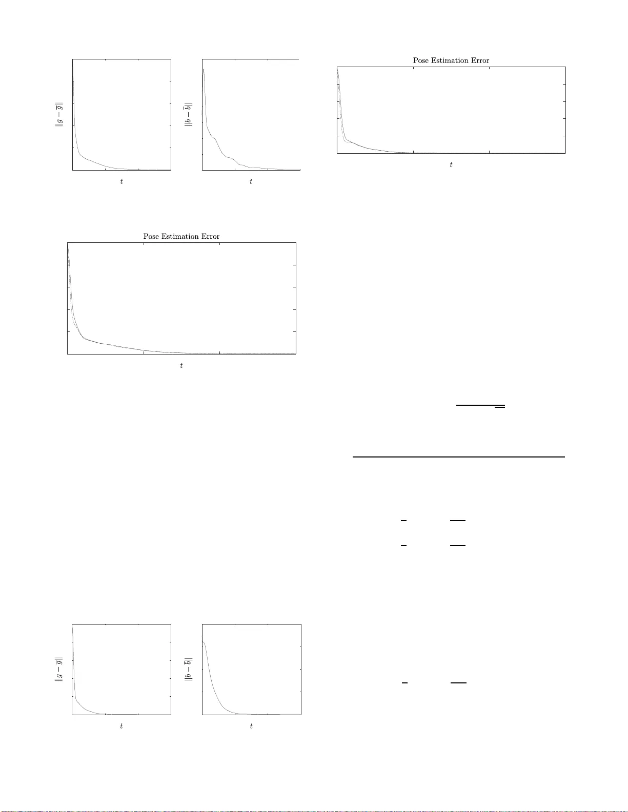
1 Design of Globally Expon entiall y Con v er gent Continuous Observe rs for V elocity Bias and State for Systems on Real Matrix Groups Dong Eui Chang Abstract —W e propose globally exponentially conv erg ent con- tinuous observ ers for in v ariant kinematic systems on finite- dimensional matrix Lie gro ups. Such an observ er estimates, from measureme nts of landmarks, vec tors and biased v elocity , both the system state a nd the unknown constant bias in velocity measureme nt, where the state belongs to the state-space Li e gro up and the velocity to the Lie algebra of the Lie group. The main technique is to embed a given system defined on a matrix Lie group into Euclidean space and build observers in th e Euclidean space. The theory is illustrated with the special Eu clidean group in thr ee dimensions. Index T erms —observe r , estimation, Lie gro up, velocity b ias I . I N T RO D U C T I O N Consider an inv ariant k inematic sy stem on a matrix Lie group G : ˙ g = g ξ with ( g , ξ ) ∈ G × g , wh e re G is em bedded in R n × n and g denotes the Lie algeb ra o f G . Suppose that the velocity ξ is measured with an additive unknown c o nstant bias as ξ m = ξ + b where b ∈ g is the constant un known bias. Suppo se also that we measure land marks and vectors such that an n × n matrix- valued sig n al A of the form A = F g or A = g − 1 F is av ailable, wher e F is an n × n invertible matrix. In this paper, we design continu ous ob ser vers that globally and exponentially estimate ( g , b ) with ξ m and A , where it is assumed th at the value of F is available. Rele vant works are listed in th e following. In [9], the authors propo sed contin uous ob servers tha t e stima te ( g , b ) with ξ m and ho mogen e ous outpu ts. The ir observers are unifo rmly locally expo nentially stable, but not globally expon e ntially stable. A similar work was done in [8 ] , wher e a gr adient- like innovation ter m was used in the observer design. Th e observers th erein are not globally exponentially stable but o nly unifor m ly loc a lly exponentially stable. Grad ient-like observers were also pro posed in [10], but these observers are not g lo bally exponentially conver gent either . T o th e best of our knowledge, our observers in the pr esent paper are th e fir st glob ally exp onentially co nvergent contin u- ous o bservers for velocity bias and state for k inematic systems on matrix Lie groups. One noticeab le difference between the ob ser vers in [8]– [ 10] and ours is that ou r obser vers are designed in R n × n × g instead of G × g , where G ⊂ R n × n , such that the Euclid ean structure o f R n × n is fu lly utilized without being con strained to the g roup structu re of G . This type of observers b uilt in Euclidean space is called g eometry- free and they have bee n widely used for SO(3 ) , e.g . [1], [11]. The paper is organized as fo llows. In Section II we p ropose various forms of globally expon entially conv ergent co ntinuou s observers for velocity bias and s tate for kinematic systems on matrix L ie grou ps. In Section III, we illustrate one of the observers proposed in Section II by app lying it to the spec ial Euclidean group SE(3) . Th e pa p er is concluded in Section IV. I I . M A I N R E S U LT S Let G b e a matrix Lie gro up that is a subgroup of GL( n ) = { A ∈ R n × n | det A 6 = 0 } , and let g den ote the Lie algebra of G . Since G is a subg roup fo GL( n ) , we may assume that g is a subalg ebra of ( R n × n , [ , ]) , where [ , ] is the usua l matrix co mmutator d e fined by [ A, B ] = AB − B A fo r all A, B ∈ R n × n . Le t π g : R n × n → g d enote the or thogon al projection onto g with respect to the Euclidea n inner pro duct h , i that is defin e d by h A, B i = tr ( A T B ) fo r A, B ∈ R n × n . Let kk d enote th e Euclidean o r Frobenius norm wh ich is defined b y k A k = p h A, A i for all A ∈ R n × n . For a squ are matrix A , λ minx ( A ) and λ max ( A ) denote the minimum eig en- value and the maximum eigenv alue of A , respectively . For any matrix A , σ min ( A ) and σ max ( A ) denote the minim u m sing ular value and the maximum sing ular value of A , respecti vely . For any A ∈ R n × n , k A k 2 = P n i =1 σ 2 i ( A ) , where σ i ( A ) ’ s are the singular values of A . W e have λ min ( A T A ) k B k 2 ≤ h AB , AB i ≤ λ max ( A T A ) k B k 2 for all A ∈ R n × m and B ∈ R m × ℓ , i.e. σ 2 min ( A ) k B k ≤ k AB k ≤ σ 2 max ( A ) k B k for all A ∈ R n × m and B ∈ R m × ℓ . Refer to [2] for more about Lie groups in the context of geom etric co ntrol and mechanics. A. Observer I The invariant kin ematic eq uation on a matrix Lie group G ⊂ R n × n is given by ˙ g = g ξ , (1) 2 where g ∈ G and ξ ∈ g . Suppo se that there is giv en an ar b itrary trajecto ry of th e system ( g ( t ) , ξ ( t )) ∈ G × g , 0 ≤ t < ∞ . W e m ake the following three assumptions. Assumption II.1. A matrix-va lu ed signa l A ( t ) ∈ R n × n is available th a t can be expr es sed as A = F g , (2) wher e F is a c onstant invertible matrix in R n × n and g ∈ G . Assumption II.2. A g - valued signal ξ m ( t ) with b ia s is avail- able a nd related to the true ξ ( t ) ∈ g of as fo llows: ξ m = ξ + b, wher e b ∈ g is an u nknown co n stant bia s vector . Assumption II .3. Ther e a r e kno wn co nstants B ξ > 0 and B b > 0 such th at k ξ ( t ) k ≤ B ξ for all t ≥ 0 and k b k ≤ B b . Ther e are n umbers L g > 0 an d U g > 0 such that L g ≤ σ min ( g ( t )) ≤ σ max ( g ( t )) ≤ U g for all t ≥ 0 , wher e th e knowledge on the values of L g and U g is not a ssume d . W e p ropose the following observer: ˙ ¯ A = ¯ Aξ m − A ¯ b + k P ( A − ¯ A ) , (3a) ˙ ¯ b = − k I π g ( A T ( A − ¯ A )) (3b) with k P > ( B ξ + B b ) and k I > 0 , wher e ( ¯ A, ¯ b ) ∈ R n × n × g is an estimate of ( A, b ) ∈ G × g . So, ( F − 1 ¯ A, ¯ b ) ∈ R n × n × g becomes an estimate of ( g , b ) ∈ G × g b y Assumption II.1. The global and exp o nentially convergent property o f this ob server is pr oven in the following theorem . Theorem II.4. Let E A = A − ¯ A, e b = b − ¯ b. Under Assumptio ns I I.1 – II. 3, for any k P > ( B ξ + B b ) an d k I > 0 there exist numbers a > 0 and C > 0 such tha t k E A ( t ) k + k e b ( t ) k ≤ C ( k E A (0) k + k e b (0) k ) e − at (4) for a ll t ≥ 0 an d all ( ¯ A (0) , ¯ b (0)) ∈ R n × n × g . Pr oof. See Appen dix. Corollary II.5. Supp ose tha t A ssumptions II.1 – II.3 hold , and let E g = g − F − 1 ¯ A, e b = b − ¯ b. Then, th er e exis t numbers a > 0 and C > 0 such tha t k E g ( t ) k + k e b ( t ) k ≤ C ( k E g (0) k + k e b (0) k ) e − at (5) for a ll t ≥ 0 an d all ( ¯ A (0) , ¯ b (0)) ∈ R n × n × g . Pr oof. Use k E g k / k F − 1 k ≤ k E A k ≤ k F kk E g k an d (4) with the constant C redefined a p propr iately . Namely , th e est imate ( F − 1 ¯ A ( t ) , ¯ b ( t )) con ver ges g lobally and expo nentially to the tru e value ( g ( t ) , b ) as t tends to ∞ . Remark II.6. W e can also build an observer that allows ¯ b to be in R n × n instead o f g . The modified observer is given by ˙ ¯ A = ¯ Aξ m − A ¯ b + k P ( A − ¯ A ) , (6a) ˙ ¯ b = − k I A T ( A − ¯ A ) , (6b) wher e ( ¯ A, ¯ b ) ∈ R n × n × R n × n . Notice that the pr o jection operator π g in (3b) is r emoved fr om (3b) to obtain (6b) . Theor em I I.4 a nd Cor ollary II.5 also ho ld for this o bserver , whose pr oof is almost iden tical to the pr oofs of Theor em II.4 and Cor ollary II .5, so it is left to the r eader . Remark II.7. Assump tion II.1 can b e r elaxed by allowing the ma trix F to be time-va rying. Mor e specifica lly , we make the following a ssumption: ther e are nu mbers ℓ min > 0 and ℓ max > 0 such that ℓ min ≤ σ min ( F ( t )) ≤ σ max ( F ( t )) ≤ ℓ max (7) for all t ≥ 0 . I n this ca se, we pr opose the follo wing observer: ˙ ¯ A = ¯ Aξ m − A ¯ b + k P ( A − ¯ A ) + ˙ F F − 1 A, ˙ ¯ b = − k I π g ( A T ( A − ¯ A )) with k P > 0 an d k I > 0 , where ( ¯ A, ¯ b ) ∈ R n × n × g is a n estimate o f ( A, b ) . It is not difficult to sh o w tha t Theorem II.4 and Cor o llary II.5 also hold fo r this observer with the relaxed assumption on F ( t ) as ab ove. Her e, the knowledge on the values o f ℓ min and ℓ max is not requir ed her e. Remark II.8. S ince the estima te F − 1 ¯ A may not lie in G in general, on e ma y need to pr oject it to G as an output of the observer althoug h F − 1 ¯ A ( t ) conver ges to g ( t ) ∈ G as t ten ds to infity . F or example, if G = SO(3) , th en the usua l polar decompo sition can be used to define a pr ojection fr om R 3 × 3 to SO(3) . Pr o jection fo r SE (3) will b e discussed in Section III. However , if one design s c ontr oller s in R n × n for an extension of (1) into R n × n as pr oposed in [4], then the dir ect use of F − 1 ¯ A in feedb ack would be fine. B. Observer II Recall the k in ematic eq uation in (1). W e now conside r a case wher e th e measuremen t matrix A is related to the true signal g ( t ) as A = g − 1 ( t ) F instead of A = F g ( t ) . Consequently , in place of Assumption I I.9, let us make the following assumption: Assumption II.9. A matrix-va lu ed signa l A ( t ) ∈ R n × n is available th a t can be expr essed as A = g − 1 F, (8) wher e F is a c onstant invertible matrix in R n × n and g ∈ G . By ( 1), A defined in ( 8) satisfies ˙ A = − ξ A. (9) Under Assumptio n s II.9, II. 2 and II. 3, we pr opose the follow- ing o b server: ˙ ¯ A = − ξ m ¯ A + ¯ bA + k P ( A − ¯ A ) , (10a) ˙ ¯ b = k I π g (( A − ¯ A ) A T ) (10b) 3 with k P > ( B ξ + B b ) and k I > 0 , wher e ( ¯ A, ¯ b ) ∈ R n × n × g is an estimate of ( A, b ) ∈ G × g . Theorem II.10 . F or the o bserver (1 0) , let E A = A − ¯ A, e b = b − ¯ b. Under Assumption s II.9, I I.2 an d II.3, for a ny k P > ( B ξ + B b ) and k I > 0 ther e exist numb ers a > 0 and C > 0 such that k E A ( t ) k + k e b ( t ) k ≤ C ( k E A (0) k + k e b (0) k ) e − at for a ll t ≥ 0 an d all ( ¯ A (0) , ¯ b (0)) ∈ R n × n × g . Pr oof. See Appen dix. Corollary II.11. Consider the observer (10) . Suppo se tha t Assumptions I I.9, II.2 and I I.3 h old, and let E g = g − F ¯ A − 1 , e b = b − ¯ b. Then, th er e exis t numbers a > 0 and C > 0 such tha t k E g ( t ) k + k e b ( t ) k ≤ C ( k E g (0) k + k e b (0) k ) e − at for a ll t ≥ 0 an d all ( ¯ A (0) , ¯ b (0)) ∈ R n × n × g . In other words, th e estimate ( F ¯ A ( t ) − 1 , ¯ b ( t )) co nverges globally a n d expo nentially to the true v alue ( g ( t ) , b ) as t tends to infinity . Remark II.12. If F ( t ) is time-varying such th at (7) is satisfied for a ll t ≥ 0 , the n (10 a) has o n ly to be modified to ˙ ¯ A = − ξ m ¯ A + ¯ bA + k P ( A − ¯ A ) + AF − 1 ˙ F while ( 10b) remains intact. W e now d eriv e from (3) various o bservers of concr ete form that estimate ( R, b ) fr om vector measureme nts. Assume tha t there is a set S = { s i , 1 ≤ i ≤ m } of m known fixed inertial vectors, wh ere each s i in S is a vector in R n , such that the rank of S is n . Assum e also tha t measurements of the vectors are m ade in the body-fixed frame a nd the set of the measured vectors is denoted b y C = { c i , 1 ≤ i ≤ m } and related to S as fo llows: c i = g − 1 s i , i = 1 , . . . , m, where F ∈ G . Let S =  s 1 · · · s m  , C =  c 1 · · · c m  (11) be n × m matrices made of the co lu mn vectors from S and C , respectively . Corollary II.13 . Let S and C be given in (1 1) . If there is a matrix W ∈ R m × n such tha t F := S W ha s rank n , th en (8 ) is satisfied b y A = C W and the o bserver (1 0) is applica ble. Pr oof. Tri vial. Remark II.14. Cor ollary II. 1 3 can be applied in several ways. F or example, the substitution o f W S T into W in Cor ollary II.13 wou ld yield F = S W S T , A = C W S T , wher e it is assumed that W is a n m × m matrix such tha t F h a s rank n . Likew ise, W in Cor ollary II.13 ca n be chosen such that F dep ends more nonlinea rly o n S . C. V ariants W e h ere propo se an o b server that is a variant of the observer (3) with A T replaced by A − 1 in (3b). Recall the kinematic equation (1), and under Assumptions I I.1 – II.3, we propo se the fo llowing new observer: ˙ ¯ A = ¯ Aξ m − A ¯ b + k P ( A − ¯ A ) , (12a) ˙ ¯ b = − k I π g ( A − 1 ( A − ¯ A )) (12b) with k P > (2 B ξ + B b ) and k I > 0 , where ( ¯ A, ¯ b ) ∈ R n × n × g is an estimate of ( A, b ) ∈ G × g . So, ( F − 1 ¯ A, ¯ b ) ∈ R n × n × g becomes an estimate of ( g , b ) ∈ G × g by Assumption I I.1. Theorem II.15 . F or the o bserver (1 2) , let E A = A − ¯ A, e b = b − ¯ b. Under Assumptions II.1 – II .3, for an y k P > (2 B ξ + B b ) and k I > 0 ther e exist n umbers a > 0 and C > 0 such that k E A ( t ) k + k e b ( t ) k ≤ C ( k E A (0) k + k e b (0) k ) e − at for a ll t ≥ 0 an d all ( ¯ A (0) , ¯ b (0)) ∈ R n × n × g . Pr oof. See Appendix . W e also pro pose a variant o f the observer (10) with A T replaced by A − 1 in (10b). Under Assumptio ns II.2, II.3 and II.9, we pro pose the f ollowing n ew observer: ˙ ¯ A = − ξ m ¯ A + ¯ bA + k P ( A − ¯ A ) , (13a) ˙ ¯ b = k I π g (( A − ¯ A ) A − 1 ) (13b) with k P > (2 B ξ + B b ) and k I > 0 , where ( ¯ A, ¯ b ) ∈ R n × n × g is an estimate of ( A, b ) ∈ G × g . So, ( F ¯ A − 1 , ¯ b ) ∈ R n × n × g becomes an estimate of ( g , b ) ∈ G × g by Assumption I I.1. Theorem II.16 . F or the o bserver (1 3) , let E A = A − ¯ A, e b = b − ¯ b. Under Assumption s II.9, I I.2 an d II.3, for a ny k P > ( B ξ + B b ) and k I > 0 the re exist numbers a > 0 and C > 0 su ch that k E A ( t ) k + k e b ( t ) k ≤ C ( k E A (0) k + k e b (0) k ) e − at for a ll t ≥ 0 an d all ( ¯ A (0) , ¯ b (0)) ∈ R n × n × g . Pr oof. Omitted since it is similar to the proof of Th e o rem II.15. Remark II.17. 1. Cor ollaries I I .5 an d II. 11 also ho ld fo r the observers (12) and ( 13) , r espectively . 2. Cor ollary II.13 and Rema rk II.14 also ho ld true for the observer (13) . 4 I I I . E X A M P L E : A P P L I C A T I O N T O SE(3) W e now illustrate the theory presen ted in Section II with the special Euclidean gr o up on R 3 . The gro up can b e expressed in homog eneous co ordinates as SE(3) =  R x 0 1  | R ∈ SO(3) , x ∈ R 3  , where SO(3) = { R ∈ R 3 × 3 | R T R = I , det R = 1 } is the special orthog o nal g roup whose L ie alg ebra is so (3) = { A ∈ R 3 × 3 | A T = − A } . It is easy to see that SE(3) is a sub group of GL(4) = { A ∈ R 4 × 4 | det A 6 = 0 } . Th e Lie alg ebra of SE(3) is then given b y se (3) =  ˆ Ω v 0 0  for some Ω ∈ R 3 , x ∈ R 3  , where the h a t map ∧ : R 3 → so (3) is defined s uch that ˆ xy = x × y fo r all x, y ∈ R 3 . In h omogen eous coo rdinates, landmark s to be m easured with sensor s are expressed in the form  x 1  , x ∈ R 3 , (14) and such vectors at infinity as the gravity or the Earth’ s magnetic field are expressed in the form  x 0  , x ∈ R 3 . (15) The orthogo nal pr ojection π se (3) : R 4 × 4 → se (3) is g iven as follows: For A ∈ R 4 × 4 giv en by A =  B x y T z  , B ∈ R 3 × 3 , x ∈ R 3 × 1 , y ∈ R 3 × 1 , z ∈ R , we h av e π se (3) ( A ) =  1 2 ( B − B T ) x 0 1 × 3 0  ∈ se (3) . Suppose tha t we m easure i n the body frame the following inertial vectors given by s 1 = ( e 1 , 1) , s 2 = ( e 2 , 1) , s 3 = ( e 3 , 1) , s 4 = ( e 1 + e 3 , 1) , s 5 = ( − e 3 , 0) , where { e 1 , e 2 , e 3 } is the standar d basis of R 3 and s 5 represents the gravity d ir ection. Suppose the measured signal matrix A ( t ) is given by A ( t ) = g ( t ) − 1 F = g ( t ) − 1 S W S T = C ( t ) W S T with F = S W S T and C ( t ) = g ( t ) − 1 S , where S =  s 1 s 2 s 3 s 4 s 5  . Here, each column in th e C ( t ) ma tr ix is wha t is measured in the bo dy-fixed f rame. For convenience, we set W = I 4 × 4 although any 4 × 4 matrix su ch that S W S T is in vertible would work f or W . Suppose that a set o f tru e trajectories ( R ( t ) , x ( t )) ∈ SE(3) and (Ω( t ) , V ( t )) ∈ R 3 × R 3 are given as fo llows: R ( t ) = exp( t ˆ e 1 ) exp( t ˆ e 3 ) exp( t ˆ e 1 ) , (16) x ( t ) = (cos t, sin t, cos t ) , (17) Ω( t ) = (1 + co s t, sin t − sin t cos t, cos t + sin 2 t ) , (18) V ( t ) = R T ( t ) ˙ x ( t ) , (19) where Ω( t ) satisfies ˆ Ω( t ) = R T ( t ) ˙ R ( t ) . Assume th at the unknown constant gyro bias b Ω and the unkn own constan t velocity bias b v are respe cti vely giv en by b Ω = (1 , 0 . 5 , − 1) , b v = (0 . 5 , − 0 . 5 , 0 . 5) . (20) W e use th e o bserver of th e form (10). Th e gains are chosen as k P = 4 an d k I = 0 . 7 5 , and the initial state of the observer is given by ¯ A (0) = ¯ g − 1 0 F where ¯ g 0 = " exp( π 2 ˆ e 1 ) 0 3 × 1 0 1 × 3 1 # and ¯ b Ω (0) = (0 , 0 , 0) , ¯ b v (0) = (0 , 0 , 0) . The simulation results are p lo tted in Fig. 1, wh ere the pose estimation err or k g ( t ) − ¯ g ( t ) k with ¯ g ( t ) := F ¯ A ( t ) − 1 ∈ R 4 × 4 , and the bias estimation error k b − ¯ b ( t ) k are plotted. It can be seen that b oth e stima tio n error s co n verge we ll to zero as theoretically p redicted. T o examine if the imag e trajectory of ¯ g ( t ) under a p rojection onto SE (3) also co n verges to g ( t ) , let us defin e a projec tio n pro j : R 4 × 4 → SE(3) as follows: for any ¯ g =  ¯ g 1 ¯ g 2 ¯ g 3 ¯ g 4  ∈ R 4 × 4 with ¯ g 1 ∈ R 3 × 3 , ¯ g 2 ∈ R 3 × 1 , ¯ g 3 ∈ R 1 × 3 , and ¯ g 4 ∈ R , pro j(¯ g ) :=  ¯ g 1 , SO(3) ¯ g 2 0 1 × 3 1  ∈ SE(3) , (21) where ¯ g 1 , SO(3) denotes the SO(3) factor in p olar d e composi- tion of ¯ g 1 . For conv enience, let ¯ g SE(3) ( t ) := pr o j( ¯ g ( t )) . The pose estimatio n err or k g ( t ) − ¯ g SE(3) ( t ) k by ¯ g SE(3) ( t ) is plotted in Fig. 2 along with the p ose estimation error k g ( t ) − ¯ g ( t ) k by ¯ g ( t ) tha t was obtained in the simulatio n. It can b e seen in the figure that ¯ g ( t ) stays very clo se to its SE(3) factor ¯ g SE(3) ( t ) , and ¯ g SE(3) ( t ) also co n verges to the tru e pose g ( t ) as time tend s to infinity . For the pu rpose of com p arison, we n ow apply the observer (13) with the same setting except the observer gains which are now chosen as k P = 4 and k I = 4 . The estimation results ar e plotted in Fig. 3. It can be seen th a t the bias estimation erro r by the o bserver (13) in Fig. 3 con verges fast w ith out overshoot in comp arison with the estimation error by ( 10) that is plotted in Fig. 1. The SE(3) part o f ¯ g ( t ) com puted by the projection (21) also conver ges well to the tr ue signal g ( t ) as shown in Fig. 4. Remark III.1. Th er e have been papers on estimatio n of po se and velocity measur ement bia s for SE(3) , e.g. [7 ], [12], [13 ] and refer enc es th e rein. A g lobally exponentia lly conver g ent hybrid (no t continuo us) observer is p r oposed in [1 2], an d a non-g lobal exponentia lly conver gent ob server is pr oposed in [13]. A gradient-like observer design on SE(3 ) with system outputs on the r eal p r ojective space was p r oposed in [7]. Refer 5 0 5 10 15 0 0.5 1 1.5 2 2.5 0 5 10 15 0 0.5 1 1.5 2 2.5 3 3.5 Fig. 1. The pose estimat ion error k g ( t ) − ¯ g ( t ) k and the veloc ity bias estimati on error k b − ¯ b ( t ) k by the observ er (10). 0 5 10 15 0 0.5 1 1.5 2 2.5 Fig. 2. T wo pose estimation errors by the observer (10 ): k g ( t ) − ¯ g ( t ) k by the observ er (solid) and k g ( t ) − ¯ g SE(3) ( t ) k by the SE(3) fa ctor ¯ g SE(3) ( t ) of ¯ g ( t ) obtaine d through the projection (21) (dash-dot ). to [6] for a glob al formulatio n of extended Kalma n filter on SE(3) for geome tric contr ol of a dr one. I V . C O N C L U S I O N W e hav e successfully designed g lobally exponentially con- vergent co ntinuou s observers for kinem atic inv ariant systems on finite-dimensio n al matrix Lie groups that estimate s tate and constant velocity bias from measur e m ents of landma r ks, vectors and biased velocity . W e have app lied the result to the special Euclid ean g r oup SE(3) and carried o ut a simu lation study to illustrate an excellent perfor m ance o f the observer for SE(3) . W e p lan to apply the result to drone contr o l [ 5] and to co mbine it with de e p neur al networks [3] . 0 5 10 15 0 0.5 1 1.5 2 2.5 0 5 10 15 0 0.5 1 1.5 2 Fig. 3. The pose estimat ion error k g ( t ) − ¯ g ( t ) k and the velocit y bias estimati on error k b − ¯ b ( t ) k by the observ er (13). 0 5 10 15 0 0.5 1 1.5 2 2.5 Fig. 4. T wo pose estimation errors by the observer (13): k g ( t ) − ¯ g ( t ) k by the observ er (solid) and k g ( t ) − ¯ g SE(3) ( t ) k by the SE(3) fa ctor ¯ g SE(3) ( t ) of ¯ g ( t ) obtaine d through the projection (21) (dash-dot ). A P P E N D I X Pr oof of Th eor em II.4 Pr oof. From (1) an d Assumptio n II. 1, A ( t ) satisfies ˙ A = Aξ . (2 2 ) By Assum ption II.2, the observer (3) can b e written as ˙ ¯ A = ¯ A ( ξ + b ) − A ¯ b + k P E A , (23a) ˙ ¯ b = − k I π g ( A T E A ) . (23b) By Assum ption II.3, there is a nu mber ǫ such that 0 < ǫ < min  H, 1 k F k U g √ k I  , where H = 4( k P − B ξ − B b ) L 2 g λ min ( F T F ) (4 k I L 2 g λ min ( F T F ) + ( k P + B b + 2 B ξ ) 2 ) U 2 g k F k 2 . The following three q uadratic functio ns of ( k E A k , k e b k ) are then all po sitive definite: V 1 ( k E A k , k e b k ) = 1 2 k E A k 2 + 1 2 k I k e b k 2 − ǫU g k F kk E A kk e b k , V 2 ( k E A k , k e b k ) = 1 2 k E A k 2 + 1 2 k I k e b k 2 + ǫU g k F kk E A kk e b k , V 3 ( k E A k , k e b k ) = ( k P − ( B ξ + B b ) − ǫk I U 2 g k F k 2 ) k E A k 2 + ǫλ min ( F T F ) L 2 g k e b k 2 − ǫ ( k P + B b + 2 B ξ ) U g k F kk E A kk e b k . Hence, th ere are numb ers α > 0 and β > 0 such that V 2 ≤ αV 1 , β V 2 ≤ V 3 . (24) Let V ( E A , e b ) = 1 2 k E A k 2 + 1 2 k I k e b k 2 + ǫ h E A , Ae b i , which satisfies V 1 ( k E A k , k e b k ) ≤ V ( E A , e b ) ≤ V 2 ( k E A k , k e b k ) (25) for all ( E A , e b ) ∈ R n × n × g by th e Cauchy-Schwarz inequ a lity and k A k = k F g k ≤ k F k U g . From (22), (23), an d the 6 assumption of the bias b b eing co nstant, it fo llows that the estimation er ror ( E A , e b ) ob eys ˙ E A = E A ( ξ + b ) − Ae b − k P E A , ˙ e b = k I π g ( A T E A ) . Along any trajectory o f th e comp osite system consisting of the rigid bod y (1) and the ob server ( 3 ), dV dt = h E A , E A ( ξ + b ) − Ae b − k P E A i + h e b , π g ( A T E A ) i + ǫ h E A ( ξ + b ) − Ae b − k P E A , Ae b i + ǫ h E A , Aξ e b i + ǫk I h E A , A π g ( A T E A ) i ≤ − ( k P − ( B ξ + B b ) − ǫk I U 2 g k F k 2 ) k E A k 2 − ǫλ min ( F T F ) L 2 g k e b k 2 + ǫ ( k P + B b + 2 B ξ ) U g k F kk E A kk e b k = − V 3 ≤ − β V 2 ≤ − β V , where th e following have been u sed : h E A , E A ( ξ + b ) i ≤ k E A k 2 ( B ξ + B b ) , h E A , Ae b i = h A T E A , e b i = h π g ( A T E A ) , e b i , h Ae b , Ae b i ≥ λ min ( F T F ) k g e b k 2 ≥ λ min ( F T F ) L 2 g k e b k 2 , h E A , A π g ( A T E A ) i = k π g ( A T E A ) k 2 ≤ k A T E A k 2 ≤ U 2 g k F k 2 k E A k 2 . Hence, V ( t ) ≤ V (0) e − β t for all t ≥ 0 an d all ( ¯ A (0) , ¯ b (0)) ∈ R n × n × g . I t fo llows fro m (24) and (25) that V 1 ( t ) ≤ V ( t ) ≤ V (0) e − β t ≤ V 2 (0) e − β t ≤ αV 1 (0) e − β t for all t ≥ 0 and all ( ¯ A (0) , ¯ b (0)) ∈ R n × n × g . Since 0 < ǫ < 1 / ( k F k U g √ k I ) , th e ma p define d by ( x 1 , x 2 ) 7→ r 1 2 x 2 1 + 1 2 k I x 2 2 − ǫU g k F k x 1 x 2 is a nor m on R 2 , where ( x 1 , x 2 ) ∈ R 2 , which is equivalent to the 1 -norm on R 2 since all norm s are equiv alent on a finite- dimensiona l vector space . Hence, V 1 ( t ) ≤ αV 1 (0) e − β t implies that th ere exists C > 0 such that (4) holds fo r all t ≥ 0 an d all ( ¯ A (0) , ¯ b (0)) ∈ R n × n × g , wh ere a = β / 2 . Pr oof of Th eor em II.10 Pr oof. By Assumption II.3, ther e is a numb er ǫ such that 0 < ǫ < min  H, L g k F k √ k I  , where H = 4( k P − B ξ − B b ) L 2 g λ min ( F T F ) (4 k I λ min ( F T F ) + ( k P + B b + 2 B ξ ) 2 U 2 g ) k F k 2 . The following three q uadratic functio ns of ( k E A k , k e b k ) are then all po sitive definite: V 1 ( k E A k , k e b k ) = 1 2 k E A k 2 + 1 2 k I k e b k 2 − ǫ L g k F kk E A kk e b k , V 2 ( k E A k , k e b k ) = 1 2 k E A k 2 + 1 2 k I k e b k 2 + ǫ L g k F kk E A kk e b k , V 3 ( k E A k , k e b k ) =  k P − ( B ξ + B b ) − ǫk I k F k 2 L 2 g  k E A k 2 + ǫλ min ( F T F ) U 2 g k e b k 2 − ǫ ( k P + B b + 2 B ξ ) L g k F kk E A kk e b k . Hence, there are n umbers α > 0 an d β > 0 such th at (24) holds. L et V ( E A , e b ) = 1 2 k E A k 2 + 1 2 k I k e b k 2 − ǫ h E A , e b A i , which satisfies (25). Since b is constant by assumption, it follows from (9) and (10) that ˙ E A = − ξ m E A + e b A − k P E A , ˙ e b = − k I π g ( E A A T ) . Along any trajectory of the comp osite system consisting of the rigid bod y (1) and the ob server ( 1 0), dV dt = h E A , − ξ m E A + e b A − k P E A i − h e b , π g ( E A A T ) i − ǫ h− ξ m E A + e b A − k P E A , e b A i + ǫ h E A , e b ξ A i + ǫk I h E A , π g ( E A A T ) A i ≤ −  k P − ( B ξ + B b ) − ǫk I k F k 2 L 2 g  k E A k 2 − ǫλ min ( F T F ) U 2 g k e b k 2 + ǫ ( k P + B b + 2 B ξ ) k F k L g k E A kk e b k = − V 3 ≤ − β V 2 ≤ − β V . The re st of the p r oof is iden tical to th e co rrespon ding part in the pr o of of Theorem I I.4, so it is omitted. Pr oof of Th eor em II.15 Pr oof. The measured matrix A = F g o beys (22) L e t E A = I − A − 1 ¯ A, e b = b − ¯ b. From ( 22) and (12), ˙ E A = E A ξ m − ξ E A − e b − k P E A ˙ e b = k I π g ( E A ) . There is an ǫ > 0 such that 0 < ǫ < min  1 √ k I , 4( k P − 2 B ξ − B b ) 4 k I + ( k P + 2 B ξ + B b ) 2  . 7 The following three q uadratic functio ns of ( k E A k , k e b k ) are then all po sitive definite: V 1 ( kE A k , k e b k ) = 1 2 kE A k 2 + 1 2 k I k e b k 2 − ǫ kE A kk e b k , V 2 ( kE A k , k e b k ) = 1 2 kE A k 2 + 1 2 k I k e b k 2 + ǫ kE A kk e b k , V 3 ( kE A k , k e b k ) = ( k P − (2 B ξ + B b ) − ǫk I ) kE A k 2 + ǫ k e b k 2 − ǫ ( k P + B b + 2 B ξ ) k E A kk e b k . Hence, there are numb ers α > 0 a nd β > 0 suc h that (24) holds. L et V ( E A , e b ) = 1 2 kE A k 2 + 1 2 k I k e b k 2 + ǫ hE A , e b i , which satisfies (25) fo r all ( E A , e b ) ∈ R n × n × g . It is easy to show that along any trajecto ry of th e compo site system consisting o f the rigid b ody (1) and the observer (1 2), ˙ V ≤ − V 3 ≤ − β V 2 ≤ − β V . As in the pro of of Th eorem II . 4, it is east to show that there are nu mbers ˜ C > 0 an d a > 0 such that kE A ( t ) k + k e b ( t ) k ≤ ˜ C ( kE A (0) k + k e b (0) k ) e − at (26) for all ( ¯ A (0) , ¯ b (0)) ∈ R n × n × g and all t ≥ 0 . Since E A = I − A − 1 ¯ A = A − 1 E A or E A = A E A = F g E A , we have σ min ( F ) L g kE A k ≤ k E A k ≤ σ max ( F ) U g kE A k . (27) It follows from (2 6) and ( 27) that there is a nu mber C > 0 such tha t k E A ( t ) k + k e b ( t ) k ≤ C ( k E A (0) k + k e b (0) k ) e − at for all ( ¯ A (0) , ¯ b (0)) ∈ R n × n × g an d all t ≥ 0 . R E F E R E N C E S [1] P . Batista, C. Silvestre, and P . Oli vei ra, “Globall y exponent ially stable cascade observers for attitude estimation, ” Contr ol E nginee ring P ractice , 20, 148 – 155, 2012. [2] A.M. Bloch, Nonholo nomic Mechani cs and Con tr ol , Sprin ger , 2003. [3] A.L. Cateri ni and D . E. Chang, Deep Neural Networks in a Mathematic al F r amew ork, Springe r , 2018. [4] D.E. Chang, “On controll er design for systems on manifolds in Eu- clide an spac e, ” J ourna l on Robust and Nonlinear Contr ol , 28(16 ), 4981 – 4998, 2018. [5] D.E. Chang and Y . Eun, “Global chartwise feedba ck linear izati on of the quadcopt er with a thrust positi vi ty preser ving dynamic exte nsion, ” IEEE T r ans. Automatic Contr ol, 62 (9), 4747 – 4752, 2017. [6] F .A. Goodarzi and T . Lee, “Global formulati on of an e xtende d Kalman filter on SE(3) for geometric control of a quadrotor UA V , ” J Intell R obot Syst , 88, 395 – 413, 2017. [7] M.-D. Hua, T . Hamel, R. Mahon y and J. Trumpf, “Gradi ent-li ke observer design on the special Euclidea n group SE(3) with system outputs on the real projecti v e space, ” In Proc. 54th IEEE Confe re nce on Decisio n and Contr o l, 2139 – 2145, Osaka J apan, 2015. [8] A. Khosravian , J. Trumpf, R. Mahony , and C. Lageman, “Bias estimation for in v aria nt systems on Lie groups with homogeneou s outputs, ” In Proc. IEEE Conf. on Decision and Contr ol , 4454 – 4460, Florence , Italy , December 201 3. [9] A. Khosravian , J. Trumpf, R. Mahony , and C. Lageman, “Observe rs for in v a riant systems on Lie groups with biased input measurements and homogeneou s outputs, ” Automatica, 55, 19 – 26, 2015. [10] C. L ageman, J. Trumpf, and R. Mahony , “Gradien t-lik e observ ers for in v a riant dynamics on a Lie group, ” IE EE T ra nsaction s on Automat ic Contr o l, 55(2), 367377, 2010. [11] P . Martin and I. Sarras, “ A global observ er for atti tude and gyro biases from vec tor measurements, ” IF AC P apersOnLine , 50-1, 15409 – 15415, 2017. [12] M. W ang and A. T ay ebi, “On the design of hybrid pose and vel ocity-b ias observe rs on Lie group SE(3), ” 2018, arXiv P re print arXiv: 1805.00897. [13] J.F . V asconcelos, R. Cunha, C. Silvestre, and P . Oli vei ra. “ A nonl inear position and atti tude observer on SE(3) using landmark measurements, ” Systems & Contr ol Let ter s, 59 (3-4), 155 – 166, 2010.