Steady-State Optimal Frequency Control for Lossy Power Grids with Distributed Communication

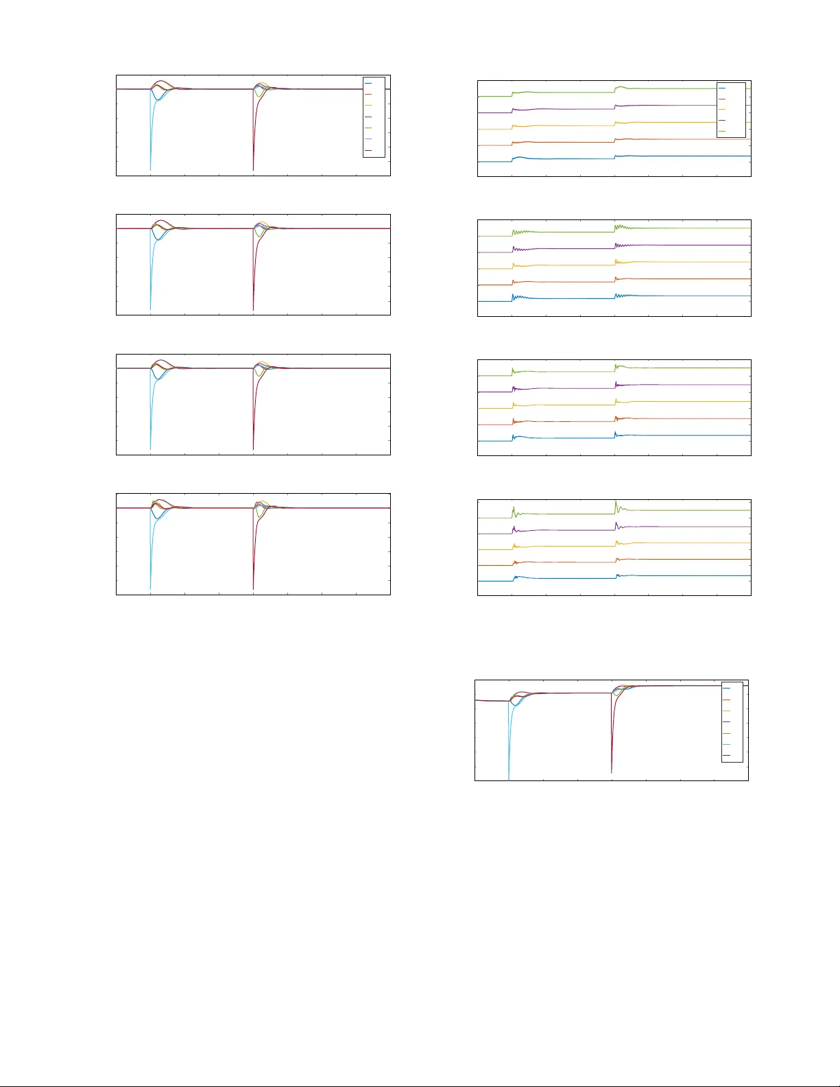
Steady-State Optimal Frequenc y Control for Lossy Po wer Grids with Distrib uted Communication Lukas K ¨ olsch, Kirtan Bhatt, Stefan Krebs, and S ¨ oren Hohmann Institute of Contr ol Systems, Karlsruhe Institute of T echnology (KIT) , Karlsruhe, Germany lukas.koelsch@kit.edu, kirtan.bhatt@student.kit.edu, stefan.krebs@kit.edu, soeren.hohmann@kit.edu Abstract —W e present a distributed and price-based control approach f or frequency r egulation in power grids with nonzer o line conductances. Both grid and controller ar e modeled as a port-Hamiltonian system, where the grid model consists of differential as well as algebraic equations. Simulations show that the resulting contr oller asymptotically stabilizes the frequency while maintaining minimum overall generation costs in steady state and being rob ust in terms of clock drifts and uncontrollable loads. Moreo ver , it is shown that active power sharing can be achieved by an appropriate choice of the cost function. Index T erms —nonlinear control, frequency regulation, dis- tributed contr ol, activ e power sharing, port-Hamiltonian systems, steady-state optimal contr ol I . I N T RO D U C T I O N A. State of Researc h Frequency control and thus regulation of the balance be- tween generation and consumption in the electrical grid has so far been the task of the transmission system operator . W ith the worldwide trend to wards more rene wable energy generation and a displacement of large con ventional power plants, there is an increasing number of small-scale generation, which raises the need for a replacement of the centralized control strategy by a distributed one. Distributing frequency regulation to sev eral agents allows to divide a complex task into se veral smaller tasks which are solved in parallel by individual agents. In addition, distributed control results in an increased robustness of the ov erall system with respect to prev enting single points of failures and attacks from outside [1]. A class of distrib uted control concepts that has recently been very popular in terms of frequency regulation and balancing is real-time dynamic pricing (see [2] for a detailed survey on current research directions). Dynamic pricing is particularly advantageous in large scale networks as it enables implicit communication of momentary imbalances via a price signal, resulting in a dynamic feedback minimization [3]–[6] of the overall costs. The price signal represents an aggregated information about current imbalances between generations and consumptions. Thus the control can be distributed based on neighbor-to-neighbor communication as well as local measure- ments and local control. The actual status of the network does not hav e to be completely known to the indi vidual agents. This work was funded by the Deutsche Forschungsgemeinschaft (DFG, German Research Foundation)—project number 360464149. Based on the formulation of a specific o verall cost function C , the distributed minimization of this cost function allows certain goals to be achiev ed at the same time, such as equal marginal prices for each agent or acti ve po wer sharing. In pre vious publications dealing with real-time dynamic pricing for frequency control of power grids, the controllers were al ways designed under the assumption that line conduc- tances are all zero [7]–[12]. Howe ver , this is an inadmissible assumption especially for distrib ution grids, see. e.g. [13]. In fact it can be sho wn by simulation that applying these controllers to the lossy A C po wer flow model alw ays leads to a synchronous frequency ω which deviates from the nominal frequency ω n . As a consequence, a practical implementation of all of these controllers would still require some kind of additional frequency restoration or secondary frequency control by a TSO. Thus a further development of distributed control algorithms is needed to provide a benefit compared to the classical hierarchy of primary , secondary , and tertiary frequency control in the lossy case. B. Main Contributions T o overcome the steady-state frequency deviation mentioned abov e, we propose an extended price-based and distributed controller , which takes into account the local nonzero conduc- tances of neighboring lines and leads to zero de viation from nominal frequency ω n . T o facilitate transient stability analysis, we represent both plant and controller as a port-Hamiltonian system, which results in a closed-loop system that is again port-Hamiltonian. Stability is then deri ved from a shifted passivity property with respect to the post-fault equilibrium. W e compare our approach with the one presented in [12] using a simulation example with both controllable and un- controllable infeeds and loads. W e sho w that stability of the closed-loop system is giv en under v arious communication topologies. Furthermore, we show the transient behavior of the closed loop under step load changes, incorrect measurements and communication failures. The remainder of this paper is organized as follows. In Section II, we gi ve some notational remarks and introduce a port-Hamiltonian formulation for a power grid with generator and load nodes which are coupled via lossy A C power lines. In Section III, we deploy a distributed price-based controller which aims at minimizing ov erall generation costs while keeping the steady-state synchronous frequency to the nominal frequency . In Section IV , we assess our approach on a test network with variable load scenarios as well as different communication topologies. Finally , in Section V , we sum up our contributions and discuss trends for future work. I I . P OW E R G R I D M O D E L A. Notational Preliminaries Positiv e semidefiniteness of a matrix is denoted by  0 , whereas element-wise nonnegati vity of a vector or matrix is denoted by ≥ 0 . V ector a = col i { a i } = col { a 1 , a 2 , . . . } is a column vector of elements a i , i = 1 , 2 , . . . and matrix A = diag i { a i } = diag { a 1 , a 2 , . . . } is a (block-)diagonal matrix of elements a i , i = 1 , 2 , . . . . The ( n × n ) -identity matrix and ( n × n ) -zero matrix are denoted by I n and 0 n , respecti vely . For all other vectors and matrices, the dimensions are either explicitly specified or they result from the context. The po wer grid is modeled by a directed graph G p = ( V , E p ) with V = V g ∪ V ` being the set of n g = |V g | generator nodes and n ` = |V ` | load nodes, respectiv ely . The physical intercon- nection is represented by the incidence matrix D p ∈ R n × m p with n = n g + n ` and m p = |E p | . Incidence matrix D p can be subdivided as follows D p =  D pg D p`  , (1) where submatrices D pg and D p` correspond to the generator and load nodes, respectiv ely . W e note j ∈ N i if node j is a neighbor of node i , i.e. j is adjacent to i in the undirected graph. A list of all parameters and variables of the power grid is giv en in T able I. B. Modeling Assumptions Follo wing the lines of [14] and [12], we make the following modeling assumptions for power grid model and controller: 1) The grid is operating around the nominal frequency ω n = 2 π · 50 Hz . 2) The grid is a balanced three-phased system and the lines are represented by its one-phase π -equi v alent circuits. 3) Subtransient dynamics of the synchronous generators are neglected. 4) Delays in communication as well as sensor and actor delays of the controllers are neglected. Howe ver , we make the following additional (relaxed) assump- tions: 5) Power lines are lossy , i.e. have nonzero conductances. 6) Loads do not have to be constant. 7) Excitation voltages of the generators do not ha ve to be constant. C. Dynamic Model of Generator Buses As in [11], each generator node is represented by a third- order synchronous generator model in local dq coordinates: ˙ θ i = ω i , i ∈ V g , (2) ˙ L i = − A i ω i + p g ,i − p `,i − p i , i ∈ V g , (3) τ U,i ˙ U i = U f ,i − U i − ( X d,i − X 0 d,i ) U − 1 i · q i , i ∈ V g . (4) T able I: List of Parameters and State V ariables of Po wer System A i positiv e generator and load damping constant B ij negati ve of susceptance of line ( i, j ) D p incidence matrix of power grid G ij negati ve of conductance of line ( i, j ) L i deviation of angular momentum from the nominal value M i ω n M i moment of inertia p i sending-end active power flow p g,i activ e power generation p `,i activ e power demand q i sending-end reactive power flow q `,i reactiv e power demand U i magnitude of transient internal voltage U f ,i magnitude of excitation voltage X d,i d-axis synchronous reactance X 0 d,i d-axis transient reactance θ i bus voltage phase angle ϑ ij bus voltage angle difference θ i − θ j Φ overall transmission losses τ U,i open-circuit transient time constant of the synchronous machine ω i deviation of bus frequency from the nominal value ω n W ithout loss of generality , yet for ease of notation, we assume that each generation p g ,i is controllable and each load p `,i and q `,i is uncontrollable. Controllable loads can easily be added as negati ve generations. Thus p g ,i are the control inputs while p `,i and q `,i act as disturbance inputs. D. Dynamic Model of Load Buses The load no de s are supposed to be uncontrollable and to hav e a frequency-dependent active power consumption, which is modeled by load damping coef ficients A i ≥ 0 and which leads to the following set of differential-algebraic equations: ˙ θ i = ω i , i ∈ V ` , (5) 0 = − A i ω i − p `,i − p i , i ∈ V ` , (6) 0 = − q `,i − q i , i ∈ V ` . (7) E. P ower Line Model The (sending-end) active and reactiv e power flows of node i ∈ V are giv en by the lossy AC power flow equations [15] p i = X j ∈N i B ij U i U j sin( θ i − θ j ) + G ii U 2 i + X j ∈N i G ij U i U j cos( θ i − θ j ) , i ∈ V , (8) q i = − X j ∈N i B ij U i U j cos( θ i − θ j ) + B ii U 2 i + X j ∈N i G ij U i U j sin( θ i − θ j ) , i ∈ V (9) with Y = G + j B being the admittance matrix. Note that by definition of the admittance matrix, G ij < 0 and B ij > 0 if nodes i and j are connected via a resistiv e-inductiv e line [15]. F . Overall Model In order to get a port-Hamiltonian state space model of the plant , i.e. the open-loop system, we chose the plant state vector as follows x p = col { ϑ , L , U g , ω `,i , U ` } (10) where for conv enience we define the angle deviation ϑ = D > p θ and the angular momenta L = col i { L i } with L i = M i · ω i , i ∈ V g . T o describe the energy stored in the power network, we choose the following positive-definite function as the plant Hamiltonian H p ( x p ) = 1 2 X i ∈V g M − 1 i L 2 i + U 2 i X d,i − X 0 d,i ! − 1 2 X i ∈V g ∪V ` B ii U 2 i − X ( i,j ) ∈E B ij U i U j cos( θ i − θ j ) + 1 2 X i ∈V ` ω 2 `,i (11) where the first row represents the (shifted) kinetic ener gy of the rotors and the magnetic energy of the generator circuits, the second row represents the magnetic energy of the transmission lines and the third row represents the local deviations of the loads from nominal frequency , i.e. the deviation from an ideal grid-supporting behavior . Combining (2)–(9), we get the following port-Hamiltonian formulation for the power grid:       ˙ ϑ ˙ L ˙ U g 0 0       =             0 D > pg 0 D > p` 0 − D pg 0 0 0 0 0 0 0 0 0 − D p` 0 0 0 0 0 0 0 0 0       | {z } J p −       0 0 0 0 0 0 A g 0 0 0 0 0 R g 0 0 0 0 0 A ` 0 0 0 0 0 b U `       | {z } R p       ∇ H p −       0 ϕ g % g ϕ ` % `       | {z } r p +       0 0 0 0 I 0 0 − b I g 0 ˆ τ U 0 0 0 0 0 − b I ` 0 0 − I 0           p g U f q ` p `     (12) with A g = diag i { A i } , i ∈ V g (13) A ` = diag i { A i } , i ∈ V ` (14) R g = diag i  X di − X 0 di τ U,i  , i ∈ V g (15) b U ` = diag i { U i } , i ∈ V ` (16) ϕ g = col i  G ii U 2 i + X j ∈N i G ij U i U j cos( ϑ ij )  , i ∈ V g (17) ϕ ` = col i  G ii U 2 i + X j ∈N i G ij U i U j cos( ϑ ij )  , i ∈ V ` (18) % g = col i  R g ,i X j ∈N i G ij U i U j sin( ϑ ij )  , i ∈ V g (19) % ` = col i  X j ∈N i G ij U i U j sin( ϑ ij )  , i ∈ V ` (20) ˆ τ U = diag i { 1 /τ U,i } , i ∈ V g (21) b I g =  I n g × n g 0 n g × n `  , (22) b I ` =  0 n ` × n g I n ` × n `  . (23) W ith J p = − J > p and R p  0 , this is a port-Hamiltonian descriptor system [16] with a nonlinear dissipativ e relation [17]. I I I . C O N T RO L L E R D E S I G N A. Contr ol Objective The aim is to minimize a certain ov erall generation cost function C ( p g ) which is assumed to be strictly con ve x. T o allo w only meaningful injection profiles p g , we add the following active po wer balance as an additional equality constraint, since it is a necessary condition for equlibrium of (12): Φ = X i ∈V g p g ,i − X i ∈V p `,i = X i ∈V G ii U 2 i + 2 · X ( i,j ) ∈E G ij U i U j cos( ϑ ij ) , (24) i.e. the surplus of energy (generation minus load) must be equal to the transmission line losses. This leads to the following constrained optimization prob- lem: min C ( p g ) sub ject to (24) (OP1) Note again that controllable loads − p g ,i with (strictly conca ve) utility functions can be modeled as generations with (strictly con ve x) generation cost functions. Follo wing the lines of [12], [14], a distrib uted representation of (OP1) is derived by transforming the scalar balance condi- tion giv en by (24) into a vector comprising of n = n g + n ` scalar equations. Equation (OP1) is fulfilled if and only if there exists some vector ν ∈ R m c , called the vector of virtual power flows [12], such that D c ν = b I > g p g − p ` − ϕ (25) with D c being an arbitrary incidence matrix of a commu- nication graph G c = ( V , E c ) with m c = |E c | edges and ϕ = col { ϕ g , ϕ ` } . As will become obvious later , the adjacency relationships of the communication graph determine which generator nodes exchange variables. A distributed representation of (OP1) is then gi ven as follows. min C ( p g ) sub ject to (25) (OP2) Since (24) as well as (25) are affine in p g , the respective optimization problems (OP1) and (OP2) are strictly con ve x. Moreov er it can be shown in [14] that (OP2) is an exact relaxation of (OP1) and thus each optimal solution of (OP2) is also optimal w .r .t. (OP1). B. Distributed Control Algorithm The constrained optimal pricing (OP2) can be achiev ed by means of a distributed control algorithm for p g . This is stated in the following proposition: Proposition 1. Let the assumptions fr om II-B be given with power grid model (12) and optimization pr oblem (OP2) . Then each equilibrium of the distributed contr ol algorithm τ g ˙ p g = −∇ C ( p g ) + b I g λ + u c , (26) τ λ ˙ λ = D c ν − b I > g p g + p ` + ϕ , (27) τ ν ˙ ν = − D > c λ (28) with τ g , τ λ , τ ν > 0 is a minimizer of (OP2) . Pr oof. Provided that Slater’ s condition is fulfilled, a necessary condition for an optimum x c := col { p g , λ , ν } of (OP2) is giv en by the KKT conditions ∇ C ( p g ) − b I g λ = 0 , (29) D > c λ = 0 , (30) − D c ν + b I > g p g − p ` − ϕ = 0 . (31) Since (OP2) is con ve x, the KKT conditions are also suf ficient. This enables the primal-dual gradient method [11], [18], [19] to be applied and results in (26)–(28). V ector u c is an additional control input and diagonal matri- ces τ g , τ λ , τ ν > 0 are controller gains, where small values for τ g , τ λ , τ ν result in a faster con ver gence with larger transient amplitudes and vice versa. Note that the distributed fashion of the controller (26)–(28) is pro vided by the fact that at each node i ∈ V g , local controller output p g ,i depends only on variables that are calculated at node i or at adjacent nodes. A port-Hamiltonian representation of (26)–(28) is giv en by ˙ x c =   0 I 0 − I 0 D c 0 − D > c 0   | {z } J c ∇ H c −   ∇ C − ϕ 0   | {z } r c +   u c p ` 0   (32) with the controller state x c = col { τ g p g , τ λ λ , τ ν ν } and the controller Hamiltonian H c ( x c ) = 1 2 x > c τ − 1 c x c (33) with τ c = diag { τ g , τ λ , τ ν } . (34) C. Closed-Loop System By choosing u c = − ω g as in [12], [14], both plant (12) and controller (32) can be interconnected in a power -preserving manner , leading to the closed-loop descriptor system: E ˙ x = ( J − R ) ∇ H − r + F u (35) with the closed-loop Hamiltonian H ( x p , x c ) = H p ( x p ) + H c ( x c ) and E = diag { I 3 n g + n + m c + m , 0 2 n ` } , (36) J =             0 I 0 0 − I 0 0 0 − I 0 D c 0 0 0 0 0 0 − D > c 0 0 0 0 0 0 0 0 0 0 D > pg 0 D > p` 0 I 0 0 − D pg 0 0 0 0 0 0 0 0 0 0 0 0 0 0 0 − D p` 0 0 0 0 0 0 0 0 0 0 0 0             , (37) R = diag { 0 n g + n + m c , R p } , (38) r = col { r c , r p } , (39) F =             0 0 0 0 0 I 0 0 0 0 0 0 0 0 − b I g ˆ τ U 0 0 0 0 − b I ` 0 − I 0             , (40) u = col { U f , q ` , p ` } . (41) It is notable that for each equlibrium x , from (26) we hav e ∇ C ( p g i ) = λ i since ω i = 0 . Moreover , from (28) it follo ws that λ ∈ k er D > c , and as D c is an incidence matrix, all elements of λ must be equal. Summing up, it follows that all marginal prices are equal at steady state, which is the economic dispatch criterion [2]. For the sake of brevity , we denote the co-state vector z = ∇ H and the dissipation vector R ( z , x ) = Rz + r . Then, (35) is a port-Hamiltonian descriptor system with nonlinear dissipation [17] E ˙ x = J z − R ( z , x ) + F u . (42) For a constant input u the corresponding equilibrium x is the solution of 0 = J z − R ( z , x ) + F u (43) Figure 1: Simulation model with fiv e generator nodes (1–5) and two load nodes (6 and 7). Solid black lines: physical interconnection via transmission lines. Dashed blue lines: Ring communication. Dotted red lines: Open ring communication. where z = ∇ H ( x ) . Since H is a conv ex and nonnegativ e function, the shifted Hamiltonian [17] H ( x ) = H ( x ) − ( x − x ) > ∇ H ( x ) − H ( x ) (44) is positi ve definite with minimum H ( x ) = 0 . Thus the shifted closed-loop dynamics, i.e. (42) minus (43), can be expressed in terms of (44) as follows: E ˙ x = J ∇ H − [ R ( z , x ) − R ( z , x )] + F [ u − u ] . (45) As a result, stability of (35) is given if the shifted passivity property [17] [ z − z ] > [ R ( z , x ) − R ( z , x )] ≥ 0 (46) is satisfied. I V . S I M U L A T I O N W e now v alidate the presented control approach by simu- lating a medium voltage power network as depicted in Fig. 1. The parameter values are partly based on those provided in [11] and are summarized in T ables II and III. Howe ver , deviating from [11], 1) Line conductances G ij are nonzero. Without loss of generality , yet for sake of simplicity , we assume constant R/X ratios η , i.e. G ij = − η · B ij for each line ( i, j ) , 2) Generator reactances and line parameters are scaled down appropriately to suit a medium-voltage distrib ution grid with a base voltage of 10 kV . The simulations were carried out in W olfram Mathematica 11.3. A. P arameterization of Input Signals and Cost Function In the following numerical examples, the po wer system is initially in a steady state with nominal frequency ω n and constant power loads p `,i . At time t = 30 s and t = 60 s , a step load change of +0 . 1 p.u. occurs at load nodes p `, 6 and p `, 7 , respectiv ely . T able II: Numerical values of the nodal parameters used in the simulations. The units of the parameters are giv en in p.u., except τ U,i which is giv en in seconds. i 1 2 3 4 5 6 7 A i 1.6 1.2 1.4 1.4 1.5 1.3 1.3 B ii -5.5 -5.5 -3.3 -3.1 -7.0 -2.0 -2.0 M i 5.2 4.0 4.5 4.2 4.4 – – X d,i 0.02 0.03 0.03 0.025 0.02 – – X 0 d,i 0.004 0.006 0.005 0.005 0.003 – – τ U,i 6.45 7.7 8.3 7.0 7.36 – – T able III: Numerical values of the line parameters used in the simulations. The units of the parameters are giv en in p.u. B 12 B 15 B 16 B 23 B 25 B 34 B 45 B 57 1 . 27 1.4 2.0 1.4 2.05 1.1 1.0 2.0 Moreov er , the ov erall cost function is chosen to be C ( p g ) = 1 2 5 X i =1 1 w i · p 2 g ,i (47) with weighting factors w 1 = 1 , w 2 = 1 . 1 , w 3 = 1 . 2 , w 4 = 1 . 3 , w 5 = 1 . 4 . The choice of a weighted sum-of-squares is con venient [20] since the above-mentioned economic dispatch criterion leads to ∇ C ( p g ,i ) = p g ,i /w i = const. for all i = 1 , . . . , 5 , i.e. active power sharing [21]. B. Numerial Results 1) Effect of communication matrix: First, we in v estigate the effect of dif ferent communication graphs on the performance of the distributed controllers. For the simulation, we employ four communication structures, namely [a] a complete communication graph (all-to-all communica- tion) [b] a communication graph identical to the physical topology of power system (solid black lines in Fig.1) [c] a ring (dashed blue lines in Fig.1) [d] an open ring (dotted red lines in Fig. 1) The R/X ratio is set to one. As seen in Fig. 2, after a certain time of about 10 seconds, all nodal frequencies return to the nominal frequency , i.e. frequency regulation is achiev ed in all four cases. Moreover , as seen in Fig. 3, injections p g ,i are equidistant for each post- fault equilibrium, i.e. active power sharing is also maintained in all four cases. The choice of D c only affects the transient behavior where a sparse communication matrix results in a slighly bigger ov ershoot of p g i after a step load change. For reasons of limited space, the communication structure for the remaining simulations is always chosen to be identical to the physical topology (communication structure [b]). 20 30 40 50 60 70 80 90 100 49 . 5 49 . 6 49 . 7 49 . 8 49 . 9 50 50 . 1 t in s f i in Hz f 1 f 2 f 3 f 4 f 5 f 6 f 7 20 30 40 50 60 70 80 90 100 49 . 5 49 . 6 49 . 7 49 . 8 49 . 9 50 50 . 1 t in s f i in Hz 20 30 40 50 60 70 80 90 100 49 . 5 49 . 6 49 . 7 49 . 8 49 . 9 50 50 . 1 t in s f i in Hz 20 30 40 50 60 70 80 90 100 49 . 5 49 . 6 49 . 7 49 . 8 49 . 9 50 50 . 1 t in s f i in Hz Figure 2: Frequency regulation after an increase in local demands p `, 6 and p `, 7 for 1) [a]–[d]. 2) Comparison to [12]: Fig. 4 shows the price-based frequency control proposed in [12] for R /X being set to one. As can be seen in Fig. 4, this results in a steady-state deviation from the nominal frequency . Evidently , the closed-loop system begins to div erge from the nominal frequency well ahead of the load increments due to the unaccounted resistiv e losses generated in the lines. Note that such a steady state deviation from nominal fre- quency always occurs in all simulations of [12] with nonzero resistiv e losses, and that this de viation from nominal frequenc y increases when resistiv e losses increase. 3) Effect of R /X ratio on closed-loop stability: In order to yield insight into stability of the closed loop, we carry out a numerical analysis of the shifted passivity property (46) for various R/X ratios. As apparent in Fig. 5, the (shifted) dissipations (46) in the system (35) tend to increase with an increase in line losses. At the same time, howe ver , they also have a more negati ve rate of 20 30 40 50 60 70 80 90 100 1 1 . 1 1 . 2 1 . 3 1 . 4 1 . 5 t in s p g ,i in p.u. p g, 1 p g, 2 p g, 3 p g, 4 p g, 5 20 30 40 50 60 70 80 90 100 1 1 . 1 1 . 2 1 . 3 1 . 4 1 . 5 t in s p g ,i in p.u. 20 30 40 50 60 70 80 90 100 1 1 . 1 1 . 2 1 . 3 1 . 4 1 . 5 t in s p g ,i in p.u. 20 30 40 50 60 70 80 90 100 1 1 . 1 1 . 2 1 . 3 1 . 4 1 . 5 t in s p g ,i in p.u. Figure 3: Optimal power injections after an increase in local demands p `, 6 and p `, 7 for 1) [a]–[d]. 20 30 40 50 60 70 80 90 100 45 . 9 46 46 . 1 46 . 2 46 . 3 46 . 4 46 . 5 t in s f i in Hz f 1 f 2 f 3 f 4 f 5 f 6 f 7 Figure 4: Steady-state deviation from nominal frequency due to neglect of line conductances in the controller design [12]. change for more resistive lines, thereby being more vulnerable to a descent into instability . This can be observed for the case R/X = 3 . Therefore, we conclude that there exists a certain R/X ratio, exceeding which the stability is no more giv en for the closed control loop. 4) Clock drifts and communication failur es: A clock drift at a particular node would manifest itself in an incorrect 20 30 40 50 60 70 80 90 100 − 1 . 5 · 10 − 3 − 7 . 5 · 10 − 4 0 7 . 5 · 10 − 4 1 . 5 · 10 − 3 t in s [ z − z ] > [ R ( z , x ) − R ( z , x )] R/X = 1 . 0 R/X = 1 . 5 R/X = 2 . 0 R/X = 3 . 0 Figure 5: Dissipations in the system for ascending R /X ratios. The system becomes unstable for R/X = 3 . 20 30 40 50 60 70 80 90 100 49 . 5 49 . 6 49 . 7 49 . 8 49 . 9 50 t in s f i in Hz f 1 f 2 f 3 f 4 f 5 f 6 f 7 20 30 40 50 60 70 80 90 100 0 . 8 1 1 . 2 1 . 4 1 . 6 1 . 8 t in s p g ,i in p.u. p g, 1 p g, 2 p g, 3 p g, 4 p g, 5 Figure 6: Performances of the distributed frequency control under a clock drift. measurement of the frequency deviation at that node, whereas a communication failure between two nodes would cut off the information flo w , so that the neighbor-to-neighbor costs and line losses can no more be calculated. T o simulate a clock drift of the controller at node 1, we assume that the measurement of ω 1 at node 1 constantly devi- ates from the actual frequency by − 1 Hz . The communication failure is modeled by eliminating the virtual power flow ν 12 between the first and the second node. As depicted in Fig. 6, simulations show that the controller is robust in terms of clock drifts and is able to restore the nominal frequency after the step load changes. Notwithstanding, activ e power sharing can no longer be achiev ed. Moreover , the communication failure leads to a steady-state synchronous frequency deviant from the nominal frequency , see Fig. 7. V . S U M M A RY A N D O U T L O O K In this paper , we propose a price-based frequency control for lossy power grids that enables distributed communication and provides zero deviation from nominal frequency . The control method can be deployed for meshed as well as radial networks in distribution level power grids. It also takes into account load nodes with uncontrollable activ e power demands and results in a differential-algebraic nonlinear power grid 20 30 40 50 60 70 80 90 100 48 . 3 48 . 4 48 . 5 48 . 6 48 . 7 48 . 8 t in s f i in Hz f 1 f 2 f 3 f 4 f 5 f 6 f 7 Figure 7: Steady-state deviation from nominal frequency due to communication failure. model that can be represented as a port-Hamiltonian descriptor system. The passivity analysis based on simulations indicates a stable system up to a certain R/X ratio in the lines. Further research includes the additional consideration of power electronics-resourced interfaces and more rigorous stability results exploiting the (shifted) passivity property of the closed- loop system. Furthermore, nodal constraints such as generation limits and operational constraints for the transmission lines shall be included in the underlying optimization problem in order to always guarantee an operation that is in compliance with all technical regulations. R E F E R E N C E S [1] S. Patnaik, J. J. P . C. Rodrigues, and A. Gawanmeh. Cyber -Physical Systems for Next-Gener ation Networks . IGI Global, 2018. [2] F . D ¨ orfler , S. Bolognani, J. W . Simpson-Porco, and S. Grammatico. Distributed control and optimization for autonomous power grids. 2019. Proc. ECC 2019 Tutorial paper. T o appear . [3] A. Jokic. Price-based optimal contr ol of electrical power systems . PhD thesis, Eindhoven Univ ersity of T echnology , 2007. [4] M. Colombino, E. Dall’Anese, and A. Bernstein. Online Optimization as a Feedback Controller: Stability and Tracking. arXiv e-prints , 1805.09877, 2018. [5] L. S. P . Lawrence, J. W . Simpson-Porco, and E. Mallada. The Optimal Steady-State Control Problem. arXiv e-prints , 1810.12892, 2018. [6] S. Menta, A. Hauswirth, S. Bolognani, G. Hug, and F . D ¨ orfler. Sta- bility of Dynamic Feedback Optimization with Applications to Power Systems. arXiv e-prints , 1810.06079, 2018. [7] E. Mallada, C. Zhao, and S. H. Low . Optimal load-side control for frequency regulation in smart grids. IEEE Tr ans. Autom. Control , 62(12):6294–6309, 2017. [8] C. Zhao, E. Mallada, S. H. Low , and J. Bialek. Distributed plug-and- play optimal generator and load control for power system frequency regulation. Int. J. Elec. P ower , 101:1–12, 2018. [9] J. K ¨ ohler , M. A. M ¨ uller , N. Li, and F . Allg ¨ ower . Real time economic dispatch for power networks: A distributed economic model predictive control approach. In Proc. IEEE Conf. Decision Contr ol , pages 6340– 6345, 2017. [10] A.-H. Mohsenian-Rad, V . W . S. W ong, J. Jatskevich, R. Schober, and A. Leon-Garcia. Autonomous demand-side management based on game- theoretic energy consumption scheduling for the future smart grid. IEEE T rans. Smart Grid , 1(3):320–331, 2010. [11] S. Trip, M. B ¨ urger , and C. De Persis. An internal model approach to (optimal) frequency regulation in power grids with time-varying voltages. Automatica , 64:240–253, 2016. [12] T . W . Stegink, C. De Persis, and A. J. van der Schaft. Stabilization of structure-preserving power networks with market dynamics. IF AC- P apersOnLine , 50:6737–6742, 2017. [13] A. Marano, J. M. M. Ortega, J. L. M. Ramos, and D. Trebolle. V oltage control of activ e distribution networks by means of dispersed generation. In CIRED 2012 W orkshop: Integration of Renewables into the Distribution Grid , pages 1–4, 2012. [14] T . Stegink, C. De Persis, and A. J. van der Schaft. A unifying energy- based approach to stability of power grids with market dynamics. IEEE T rans. Autom. Control , 62(6):2612–2622, 2017. [15] J. Machowski, J. W . Bialek, and J. R. Bumby . P ower system dynamics: Stability and contr ol . Wile y , 2012. [16] C. Beattie, V . Mehrmann, H. Xu, and H. Zwart. Port-Hamiltonian descriptor systems. arXiv e-prints , 1705.09081, 2017. [17] A. J. van der Schaft. L2-Gain and P assivity T echniques in Nonlinear Contr ol . Springer International Publishing, Cham, 2017. [18] A. Jokic, M. Lazar, and P . P . J. van den Bosch. On constrained steady- state regulation: Dynamic kkt controllers. IEEE T rans. Autom. Contr ol , 54(9):2250–2254, 2009. [19] T . Stegink, C. De Persis, and A. J. van der Schaft. Port-hamiltonian formulation of the gradient method applied to smart grids. IF AC- P apersOnLine , 48(13):13–18, 2015. [20] P . Monshizadeh, C. De Persis, T . Stegink, N. Monshizadeh, and A. J. v an der Schaft. Stability and frequency re gulation of in verters with capacitiv e inertia. In Proc. IEEE Conf. Decision Contr ol , pages 5696–5701, 2017. [21] J. Schiffer . Stability and P ower Sharing in Micr ogrids . PhD thesis, TU Berlin, 2015.