Deep Model Reference Adaptive Control

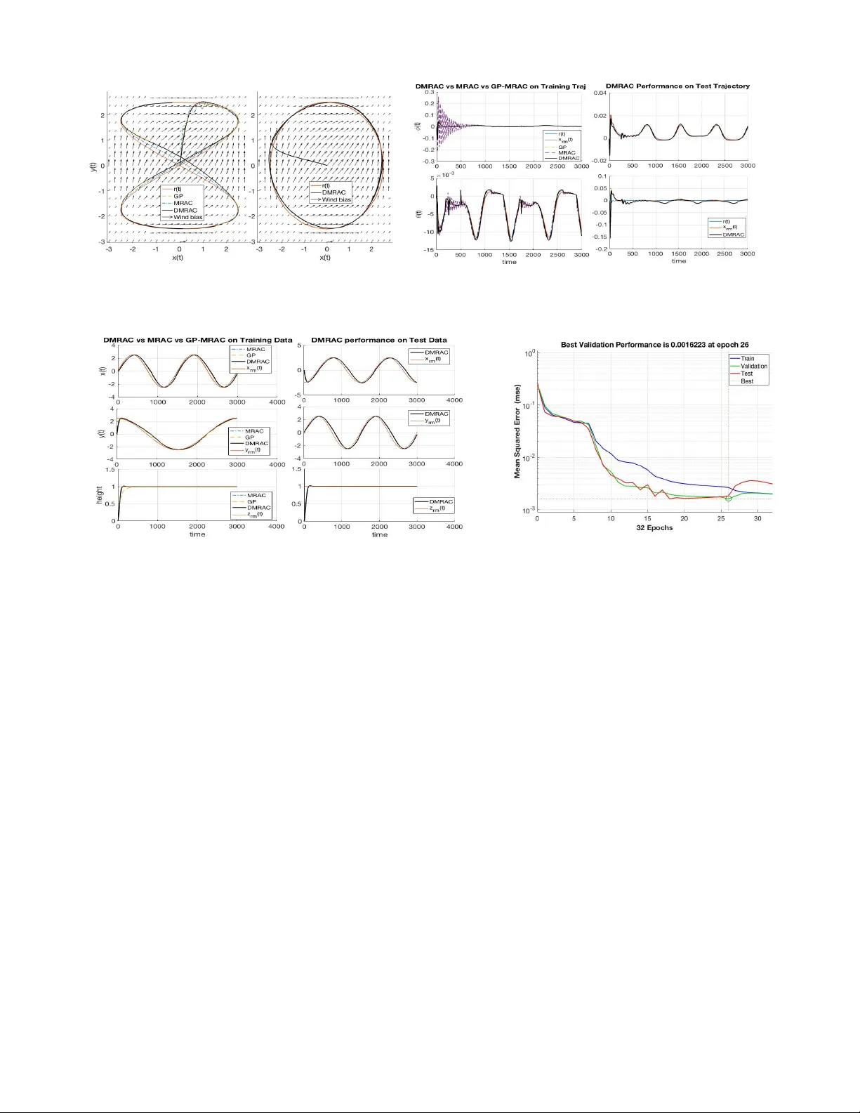
Deep Model Reference Adapti ve Control Girish Joshi and Girish Cho wdhary Abstract — W e present a new neuroadaptive architectur e: Deep Neural Network based Model Reference Adaptive Con- trol (DMRA C). Our architecture utilizes the power of deep neural network representations f or modeling significant non- linearities while marrying it with the boundedness guarantees that characterize MRA C based controllers. W e demonstrate through simulations and analysis that DMRA C can subsume pre viously studied lear ning based MRA C methods, such as concurrent learning and GP-MRA C. This makes DMRA C a highly powerful architectur e for high-performance control of nonlinear systems with long-term learning properties. I . I N T RO D U C T I O N Deep Neural Networks (DNN) ha ve lately sho wn tremen- dous empirical performance in man y applications and v arious fields such as computer vision, speech recognition, trans- lation, natural language processing, Robotics, Autonomous driving and many more [1]. Unlike their counterparts such as shallow networks with Radial Basis Function features [2], [3], deep networks learn features by learning the weights of nonlinear compositions of weighted features arranged in a directed acyclic graph [4]. It is now pretty clear that deep neural networks are outshining other classical machine- learning techniques [5]. Le veraging these successes, there hav e been many exciting new claims regarding the control of complex dynamical systems in simulation using deep reinforcement learning [6]. Howe ver , Deep Reinforcement Learning (D-RL) methods typically do not guarantee stability or ev en the boundedness of the system during the learning transient. Hence despite significant simulation success, D-RL has seldomly been used in safety-critical applications. D-RL methods often make the er godicity assumption, requiring that there is a nonzero probability of the system states returning to the origin. In practice, such a condition is typically enforced by resetting the simulation when a failure occurs. Unfortunately , howe ver , real-world systems do not hav e this reset option. Unlike, D-RL much effort has been dev oted in the field of adaptive control to ensuring that the system stays stable during learning. Model Reference Adaptiv e Control (MRA C) is one such leading method for adapti ve control that seeks to learn a high-performance control policy in the presence of signif- icant model uncertainties [7]–[9]. The key idea in MRA C *Supported by the Laboratory Directed Research and Development pro- gram at Sandia National Laboratories, a multi-mission laboratory managed and operated by National T echnology and Engineering Solutions of Sandia, LLC., a wholly o wned subsidiary of Honeywell International, Inc., for the U.S. Department of Energy’ s National Nuclear Security Administration under contract DE-NA-0003525. Authors are with Coordinated Science Laboratory , Univ ersity of Illinois, Urbana-Champaign, IL, USA girishj2@illinois.edu,girishc@illinois.edu is to find an update law for a parametric model of the uncertainty that ensures that the candidate L yapunov function is non-increasing. Many update laws hav e been proposed and analyzed, which include b ut not limited to σ -modification [10], e -modification [11], and projection-based updates [9]. More modern laws extending the classical parametric setting include ` 1 -adaptiv e control [12] and concurrent learning [13] hav e also been studied. A more recent work introduced by the author is the Gaussian Process Model Reference Adaptive Control (GP- MRA C), which utilizes a GP as a model of the uncertainty . A GP is a Bayesian nonparametric adaptiv e element that can adapt both its weights and the structure of the model in response to the data. The authors and others have shown that GP-MRA C has strong long-term learning properties as well as high control performance [14], [15]. Howe ver , GPs are “shallow” machine learning models, and do not utilize the po wer of learning complex features through compositions as deep networks do (see II-A). Hence, one wonders whether the power of deep learning could lead to even more powerful learning based MRA C architectures than those utilizing GPs. In this paper , we address this critical question: Ho w can MRA C utilize deep netw orks while guaranteeing stability? T o wards that goal, our contributions are as follows: a) W e dev elop an MRA C architecture that utilizes DNNs as the adaptiv e element; b) W e propose an algorithm for the online update of the weights of the DNN by utilizing a dual time- scale adaptation scheme. In our algorithm, the weights of the outermost layers are adapted in real time, while the weights of the inner layers are adapted using batch updates c) W e dev elop theory to guarantee Uniform Ultimate Boundedness (UUB) of the entire DMRA C controller; d) W e demonstrate through simulation results that this architecture has desirable long term learning properties. W e demonstrate ho w DNNs can be utilized in stable learning schemes for adapti ve control of safety-critical sys- tems. This provides an alternative to deep reinforcement learning for adaptiv e control applications requiring stability guarantees. Furthermore, the dual time-scale analysis scheme used by us should be generalizable to other DNN based learning architectures, including reinforcement learning. I I . B AC K G RO U N D A. Deep Networks and F eatur e spaces in machine learning The key idea in machine learning is that a giv en function can be encoded with weighted combinations of featur e v ector Φ ∈ F , s.t Φ( x ) = [ φ 1 ( x ) , φ 2 ( x ) , ..., φ k ( x )] T ∈ R k , and W ∗ ∈ R k × m a v ector of ‘ideal’ weights s.t k y ( x ) − W ∗ T Φ( x ) k ∞ <  ( x ) . Instead of hand picking features, or relying on polynomials, Fourier basis functions, comparison- type features used in support vector machines [16], [17] or Gaussian Processes [18], DNNs utilize composite functions of features arranged in a directed acyclic graphs, i.e. Φ( x ) = φ n ( θ n − 1 , φ n − 1 ( θ n − 2 , φ n − 2 ( ... )))) where θ i ’ s are the layer weights. The univ ersal approximation property of the DNN with commonly used feature functions such as sigmoidal, tanh, and RELU is proved in the work by Hornik’ s [19] and shown empirically to be true by recent results [20]–[22]. Hornik et al. argued the network with at least one hidden layer (also called Single Hidden Layer (SHL) network) to be a uni versal approximator . Howe ver , empirical results show that the networks with more hidden layers show better generalization capability in approximating complex function. While the theoretical reasons behind better generalization ability of DNN are still being in vestigated [23], for the purpose of this paper, we will assume that it is indeed true, and focus our efforts on designing a practical and stable control scheme using DNNs. B. Neur o-adaptive contr ol Neural networks in adaptive control hav e been studied for a very long time. The seminal paper by Lewis [24] utilized T aylor series approximations to demonstrate uniform ultimate boundedness with a single hidden neural network. SHL netw orks are nonlinear in the parameters; hence, the analysis previously introduced for linear in parameter , radial basis function neural networks introduced by Sanner and Slotine does not directly apply [2]. The back-propagation type scheme with non-increasing L yapunov candidate as a constraint, introduced in Lewis’ work has been widely used in Neuro-adapti ve MRAC. Concurrent Learning MRAC (CL-MRA C) is a method for learning based neuro-adaptiv e control dev eloped by the author to improve the learning properties and provide exponential tracking and weight error con ver gence guarantees. Howe ver , similar guarantees ha ve not been av ailable for SHL networks. There has been much work, towards including deeper neural networks in control; howe ver , strong guarantees like those in MRAC on the closed-loop stability during online learning are not available. In this paper , we propose a dual time-scale learning approach which ensures such guarantees. Our approach should be generalizable to other applications of deep neural networks, including policy gradient Reinforcement Learning (RL) [25] which is very close to adapti ve control in its formulation and also to more recent work in RL for control [26]. C. Stochastic Gradient Descent and Batch T raining W e consider a deep network model with parameters θ , and consider the problem of optimizing a non con vex loss function L ( Z, θ ) , with respect to θ . Let L ( Z, θ ) is defined as av erage loss ov er M training sample data points. L ( Z, θ ) = 1 M M X i =1 ` ( Z i , θ ) (1) where M denotes the size of sample training set. For each sample size of M , the training data are in form of M -tuple Z M = ( Z 1 , Z 2 , . . . Z M ) of Z − valued random v ariables drawn according to some unknown distribution P ∈ P . Where each Z i = { x i , y i } are the labelled pair of input and target values. For each P the expected loss can be computed as E p ( ` ( Z, θ )) . The abov e empirical loss (1) is used as proxy for the expected value of loss with respect to the true data generating distribution. Optimization based on the Stochastic Gradient Descent (SGD) algorithm uses a stochastic approximation of the gradient of the loss L ( Z, θ ) obtained over a mini-batch of M training examples dra wn from b uffer B . The resulting SGD weight update rule θ k +1 = θ k − η 1 M M X i =1 ∇ θ ` ( Z i , θ k ) (2) where η is the learning rate. Further details on generating i.i.d samples for DNN learning and the training details of network are provided in section IV. I I I . S Y S T E M D E S C R I P T I O N This section discusses the formulation of model reference adaptiv e control (see e.g. [7]). W e consider the follo wing system with uncertainty ∆( x ) : ˙ x ( t ) = Ax ( t ) + B ( u ( t ) + ∆( x )) (3) where x ( t ) ∈ R n , t > 0 is the state v ector , u ( t ) ∈ R m , t > 0 is the control input, A ∈ R n × n , B ∈ R n × m are known system matrices and we assume the pair ( A, B ) is controllable. The term ∆( x ) : R n → R m is matched system uncertainty and be Lipschitz continuous in x ( t ) ∈ D x . Let D x ⊂ R n be a compact set and the control u ( t ) is assumed to belong to a set of admissible control inputs of measurable and bounded functions, ensuring the e xistence and uniqueness of the solution to (3). The reference model is assumed to be linear and therefore the desired transient and steady-state performance is defined by a selecting the system eigen values in the negativ e half plane. The desired closed-loop response of the reference system is given by ˙ x rm ( t ) = A rm x rm ( t ) + B rm r ( t ) (4) where x rm ( t ) ∈ D x ⊂ R n and A rm ∈ R n × n is Hurwitz and B rm ∈ R n × r . Furthermore, the command r ( t ) ∈ R r denotes a bounded, piece wise continuous, reference signal and we assume the reference model (4) is bounded input-bounded output (BIBO) stable [7]. The true uncertainty ∆( x ) in unknown, but it is assumed to be continuous ov er a compact domain D x ⊂ R n . A Deep Neural Networks (DNN) have been widely used to represent a function when the basis vector is not kno wn. Using DNNs, a non linearly parameterized network estimate of the uncertainty can be written as ˆ ∆( x ) , θ T n Φ( x ) , where θ n ∈ R k × m are network weights for the final layer and Φ( x ) = φ n ( θ n − 1 , φ n − 1 ( θ n − 2 , φ n − 2 ( ... )))) , is a k dimen- sional feature vector which is function of inner layer weights, activ ations and inputs. The basis vector Φ( x ) ∈ F : R n → R k is considered to be Lipschitz continuous to ensure the existence and uniqueness of the solution (3). A. T otal Contr oller The aim is to construct a feedback law u ( t ) , t > 0 , such that the state of the uncertain dynamical system (3) asymptotically tracks the state of the reference model (4) despite the presence of matched uncertainty . A tracking control law consisting of linear feedback term u pd = K x ( t ) , a linear feed-forward term u crm = K r r ( t ) and an adaptive term ν ad ( t ) form the total controller u = u pd + u crm − ν ad (5) The baseline full state feedback and feed-forward controller is designed to satisfy the matching conditions such that A rm = A − B K and B rm = B K r . For the adaptiv e controller ideally we want ν ad ( t ) = ∆( x ( t )) . Since we do not have true uncertainty information, we use a DNN estimate of the system uncertainties in the controller as ν ad ( t ) = ˆ ∆( x ( t )) . B. Deep Model Refer ence Generative Network (D-MRGEN) for uncertainty estimation Unlike traditional MRAC or SHL-MRA C weight update rule, where the weights are moved in the direction of diminishing tracking error , training a deep Neural network is much more in volved. Feed-Forward networks like DNNs are trained in a supervised manner ov er a batch of i.i.d data. Deep learning optimization is based on Stochastic Gradient Descent (SGD) or its variants. The SGD update rule relies on a stochastic approximation of the expected v alue of the gradient of the loss function over a training set or mini- batches. T o train a deep network to estimate the system uncer- tainties, unlik e MRA C we need labeled pairs of state-true uncertainties { x ( t ) , ∆( x ( t )) } i.i.d samples. Since we do not hav e access to true uncertainties ( ∆( x ) ), we use a generative network to generate estimates of ∆( x ) to create the labeled targets for deep network training. F or details of the generati ve network architecture in the adaptiv e controller, please see [15]. This generativ e network is deri ved from separating the DNN into inner feature layer and the final output layer of the network. W e also separate in time-scale the weight updates of these two parts of DNN. T emporally separated weight update algorithm for the DNN, approximating system uncertainty is presented in more details in further sections. C. Online P arameter Estimation law The last layer of DNN with learned features from inner layer forms the Deep-Model Reference Generati ve Network (D-MRGeN). W e use the MRAC learning rule to update pointwise in time, the weights of the D-MRGeN in the direction of achieving asymptotic tracking of the reference model by the actual system. Since we use the D-MRGeN estimates to train DNN model, we first study the admissibility and stability character- istics of the generativ e model estimate ∆ 0 ( x ) in the controller (5). T o achie ve the asymptotic con ver gence of the reference model tracking error to zero, we use the D-MRGeN estimate in the controller (5) as ν ad = ∆ 0 ( x ) ν ad ( t ) = W T φ n ( θ n − 1 , φ n − 1 ( θ n − 2 , φ n − 2 ( ... )))) (6) T o differentiate the weights of D-MRGeN from last layer weights of DNN “ θ n ”, we denote D-MRGeN weights as “ W ”. Assumption 1: Appealing to the uni versal approximation property of Neural Networks [27] we ha ve that, for ev ery giv en basis functions Φ( x ) ∈ F there exists unique ideal weights W ∗ ∈ R k × m and  1 ( x ) ∈ R m such that the following approximation holds ∆( x ) = W ∗ T Φ( x ) +  1 ( x ) , ∀ x ( t ) ∈ D x ⊂ R n (7) F act 1: The network approximation error  1 ( x ) is upper bounded, s.t ¯  1 = sup x ∈D x k  1 ( x ) k , and can be made arbitrarily small given sufficiently large number of basis functions. The reference model tracking error is defined as e ( t ) = x rm ( t ) − x ( t ) . Using (3) & (4) and the controller of form (5) with adaptation term ν ad , the tracking error dynamics can be written as ˙ e ( t ) = ˙ x rm ( t ) − ˙ x ( t ) (8) ˙ e ( t ) = A rm e ( t ) + ˜ W T Φ( x ) +  1 ( x ) (9) where ˜ W = W ∗ − W is error in parameter . The estimate of the unknown true network parameters W ∗ are calculated on-line using the weight update rule (10); correcting the weight estimates in the direction of minimizing the instantaneous tracking error e ( t ) . The resulting update rule for network weights in estimating the total uncertainty in the system is as follows ˙ W = Γ pr oj ( W , Φ( x ) e ( t ) 0 P ) W (0) = W 0 (10) where Γ ∈ R k × k is the learning rate and P ∈ R n × n is a positive definite matrix. For gi ven Hurwitz A rm , the matrix P ∈ R n × n is a positive definite solution of L yapunov equation A T rm P + P A rm + Q = 0 for given Q > 0 Assumption 2: For uncertainty parameterized by unknown true weight W ∗ ∈ R k × m and known nonlinear basis Φ( x ) , the ideal weight matrix is assumed to be upper bounded s.t k W ∗ k ≤ W b . This is not a restrictive assumption. 1) L yapunov Analysis: The on-line adaptiv e identifica- tion law (10) guarantees the asymptotic con vergence of the tracking errors e ( t ) and parameter error ˜ W ( t ) under the condition of persistency of e xcitation [7], [28] for the structured uncertainty . Similar to the results by Lewis for SHL networks [29], we show here that under the assumption of unstructured uncertainty represented by a deep neural network, the tracking error is uniformly ultimately bounded (UUB). W e will pro ve the following theorem under switching feature vector assumption. Theor em 1: Consider the actual and reference plant model (3) & (4). If the weights parameterizing total uncertainty in the system are updated according to identification law (10) Then the tracking error k e k and error in netw ork weights k ˜ W k are bounded for all Φ ∈ F . Pr oof: The feature vectors belong to a function class characterized by the inner layer network weights θ i s.t Φ ∈ F . W e will prov e the L yapunov stability under the assumption that inner layer of DNN presents us a feature which results in the worst possible approximation error compared to network with features before switch. For the purpose of this proof let Φ( x ) denote feature before switch and ¯ Φ( x ) be the feature after switch. W e define the error  2 ( x ) as,  2 ( x ) = sup ¯ Φ ∈F   W T ¯ Φ( x ) − W T Φ( x )   (11) Similar to F act-1 we can upper bound the error  2 ( x ) as ¯  2 = sup x ∈D x k  2 ( x ) k . By adding and subtracting the term W T ¯ Φ( x ) , we can rewrite the error dynamics (9) with switched basis as, ˙ e ( t ) = A rm e ( t ) + W ∗ T Φ( x ) − W T Φ( x ) + W T ¯ Φ( x ) − W T ¯ Φ( x ) +  1 ( x ) (12) From Assumption-1 we know there exists a W ∗ ∀ Φ ∈ F . Therefore we can replace W ∗ T Φ( x ) by W ∗ T ¯ Φ( x ) and rewrite the Eq-(12) as ˙ e ( t ) = A rm e ( t ) + ˜ W T ¯ Φ( x ) + W T ( ¯ Φ( x ) − Φ( x )) +  1 ( x ) (13) For arbitrary switching, for any ¯ Φ( x ) ∈ F , we can prov e the boundedness by considering worst possible approximation error and therefore can write, ˙ e ( t ) = A rm e ( t ) + ˜ W T ¯ Φ( x ) +  2 ( x ) +  1 ( x ) (14) Now lets consider V ( e, ˜ W ) > 0 be a differentiable, positi ve definite radially unbounded L yapunov candidate function, V ( e, ˜ W ) = e T P e + ˜ W T Γ − 1 ˜ W 2 (15) The time deriv ativ e of the lyapunov function (15) along the trajectory (14) can be ev aluated as ˙ V ( e, ˜ W ) = ˙ e T P e + e T P ˙ e − ˜ W T Γ − 1 ˙ ˆ W (16) Using (14) & (10) in (16), the time deriv ativ e of the lyan- punov function reduces to ˙ V ( e, ˜ W ) = − e T Qe + 2 e T P  ( x ) (17) where  ( x ) =  1 ( x ) +  2 ( x ) and ¯  = ¯  1 + ¯  2 . Hence ˙ V ( e, ˜ W ) ≤ 0 outside compact neighborhood of the origin e = 0 , for some sufficiently large λ min ( Q ) . k e ( t ) k ≥ 2 λ max ( P )¯  λ min ( Q ) (18) Using the BIBO assumption x rm ( t ) is bounded for bounded reference signal r ( t ) , thereby x ( t ) remains bounded. Since V ( e, ˜ W ) is radially unbounded the result holds for all x (0) ∈ D x . Using the fact, the error in parameters ˜ W are bounded through projection operator [30] and further using L yapunov Fig. 1: DMRAC training and controller details theory and Barbalats Lemma [31] we can sho w that e ( t ) is uniformly ultimately bounded in vicinity to zero solution. From Theorem-1 & (9) and using system theory [32] we can infer that as e ( t ) → 0 , ∆ 0 ( x ) → ∆( x ) in point- wise sense. Hence D-MRGeN estimates y τ = ∆ 0 ( x τ ) are admissible target values for training DNN features over the data Z M = {{ x τ , y τ }} M τ =1 . The details of DNN training and implementation details of DMRAC controller is presented in the following section. I V . A D AP T I V E C O N T RO L U S I N G D E E P N E T S ( D M R A C ) The DNN architecture for MRA C is trained in two steps. W e separate the DNN into two networks, as shown in Fig- 1. The faster learning outer adaptive network and slo wer deep feature network. DMRA C learns underlying deep fea- ture vector to the system uncertainty using locally exciting uncertainty estimates obtained using a generative network. Between successiv e updates of the inner layer weights, the feature provided by the inner layers of the deep network is used as the fixed feature vector for outer layer adapti ve network update and ev aluation. The algorithm for DNN learning and DMRAC controller is provided in Algorithm-1. Through this architecture of mixing two-time scale learning, we fuse the benefits of DNN memory through the retention of relev ant, exciting features and robustness, boundedness guarantee in reference tracking. This key feature of the presented framew ork ensures rob ustness while guaranteeing long term learning and memory in the adaptiv e network. Also as indicated in the controller architecture Fig-1 we can use contextual state ‘ c i ’ other than system state x ( t ) to extract relev ant features. These contextual states could be relev ant model information not captured in system states. For example, for an aircraft system, vehicle parameters like pitot tube measurement, the angle of attack, engine thrust, and so on. These contextual states can extract features which help in decision making in case of faults. The w ork on DMRA C with contextual states will be dealt with in the follow on work. The DNN in DMRA C controller is trained over training dataset Z M = { x i , ∆ 0 ( x i ) } M i =1 , where the ∆ 0 ( x i ) are D- MRGeN estimates of the uncertainty . The training dataset Z M is randomly drawn from a larger data buffer B . Not ev ery pair of data { x i , ∆ 0 ( x i ) } from D-MRGeN is added to the training buf fer B . W e qualify the input-target pair based on kernel independence test such that to ensure that we collect locally e xciting independent information which provides a sufficiently rich representation of the operating domain. Since the state-uncertainty data is the realization of a Marko v process, such a method for qualifying data to be sufficiently independent of previous data-points is necessary . The algorithm details to qualify and add a data point to the buf fer is provided in detail in subsection IV -B. A. Details of Deep F eatur e T raining using D-MRGeN This section provides the details of the DNN training over data samples observed over n-dimensional input subspace x ( t ) ∈ X ∈ R n and m-dimensional targets subspace y ∈ Y ∈ R m . The sample set is denoted as Z where Z ∈ X × Y . W e are interested in the function approximation tasks for DNN. The function f θ is the learned approximation to the model uncertainty with parameters θ ∈ Θ , where Θ is the space of parameters, i.e. f θ : R n → R m . W e assume a training data buf fer B has p max training examples, such that the set Z p max = { Z i | Z i ∈ Z } p max i =1 = { ( x i , y i ) ∈ X × Y } p max i =1 . The samples are independently drawn from the buf fer B ov er probability distribution P . The hypothesis set, which consist of all possible functions f θ is denoted as H . Therefore a learning algorithm A (in our case SGD) is a mapping from A : Z p max → H The loss function, which measures the discrepancy be- tween true target y and algorithm’ s estimated target function value f θ is denoted by L ( y , f θ ( x )) . Specific to work pre- sented in this paper, we use a ` 2 -norm between values i.e. E p ( ` ( y , f θ ( x ))) = E P ( k y i − f θ ( x i ) k 2 ) as loss function for DNN training. The empirical loss (1) is used to approximate the loss function since the distribution P is unknown to learning algorithm. The weights are updated using SGD in the direction of negati ve gradient of the loss function as gi ven in (2). Unlike the conv entional DNN training where the true target values y ∈ Y are a vailable for e very input x ∈ X , in DMRA C true system uncertainties as the labeled targets are not av ailable for the network training. W e use the part of the network itself (the last layer) with pointwise weight updated according to MRAC-rule as the generati ve model for the data. The D-MRGeN uncertainty estimates y = W T Φ( x, θ 1 , θ 2 , . . . θ n − 1 ) = ∆ 0 ( x ) along with inputs x i make the training data set Z p max = { x i , ∆ 0 ( x i ) } p max i =1 . Note that we use interchangably x i and x ( t ) as discrete representation of continuous state vector for DNN training. The main purpose of DNN in the adaptiv e network is to extract relev ant features of the system uncertainties, which otherwise is very tedious to obtain without the limits on the domain of operation. W e also demonstrate empirically , that the DNN features trained over past i.i.d representati ve data retains the memory of the past instances and can be used as the frozen feed- forward network over similar reference tracking tasks with- out loss of the guaranteed tracking performance. B. Method for Recor ding Data using MRGeN for DNN T raining In statistical inference, implicitly or explicitly one always assume that the training set Z M = { x i , y i } M i =1 is composed on M-input-target tuples that are independently drawn from buf fer B over same joint distribution P ( x, y ) . The i.i.d assumption on the data is required for rob ustness, consistency of the network training and for bounds on the generalization error [33], [34]. In classical generalization proofs one such condition is that 1 p max X T X → γ as p max → ∞ , where X denotes the design matrix with ro ws Φ T i . The i.i.d assumption implies the above condition is fulfilled and hence is sufficient but not necessary condition for consistency and error bound for generati ve modeling. The key capability brought about by DMRAC is a relev ant feature extraction from the data. Feature extraction in DNN is achiev ed by using recorded data concurrently with current data. The recorded data include the state x i , feature vector Φ( x i ) and associated D-MRGeN estimate of the uncertainty ∆ 0 ( x i ) . For a giv en ζ tol ∈ R + a simple way to select the instantaneous data point { x i , ∆ 0 ( x i ) } for recording is to required to satisfy following condition γ i = k Φ( x i ) − Φ p k 2 k Φ( x i ) k ≥ ζ tol (19) Where the index p is over the data points in buf fer B . The abov e method ascertains only those data points are selected for recording that are suf ficiently different from all other previously recorded data points in the buf fer . Since the buf fer B is of finite dimension, the data is stored in a cyclic manner . As the number of data points reaches the b uf fer budget, a ne w data is added only upon one existing data point is removed such that the singular v alue of the buf fer is maximized. The singular v alue maximization approach for the training data buf fer update is provided in [35]. V . S A M P L E C O M P L E X I T Y A N D S T A B I L I T Y A N A L Y S I S F O R D M R AC In this section, we present the sample complexity results, generalization error bounds and stability guarantee proof for DMRA C. W e sho w that DMRAC controller is characterized by the memory of the features learned over pre viously observed training data. W e further demonstrate in simulation that when a trained DMRA C is used as a feed-forward net- work with frozen weights, can still produce bounded tracking performance on reference tracking tasks that are related but reasonably different from those seen during network training. W e ascribe this property of DMRA C to the very low generalization error bounds of the DNN. W e will prove this property in two steps. Firstly we will prove the bound on the generalization error of DNN using L yapunov theory such that we achieve an asymptotic con ver gence in tracking error . Further , we will sho w information theoretically the lower bound on the number of independent samples we need to Algorithm 1 D-MRA C Controller T raining 1: Input: Γ , η , ζ tol , p max 2: while New measurements are av ailable do 3: Update the D-MRGeN weights W using Eq:(10) 4: Compute y τ +1 = ˆ W T Φ( x τ +1 ) 5: Giv en x τ +1 compute γ τ +1 by Eq-(19). 6: if γ τ +1 > ζ tol then 7: Update B : Z (:) = { x τ +1 , y τ +1 } and X : Φ( x τ +1 ) 8: if |B | > p max then 9: Delete element in B by SVD maximization [35] 10: end if 11: end if 12: if |B | ≥ M then 13: Sample a mini-batch of data Z M ⊂ B 14: T rain the DNN network over mini-batch data using Eq-(2) 15: Update the feature vector Φ for D-MRGeN network 16: end if 17: end while train through before we can claim the DNN generalization error is well belo w a determined lower le vel gi ven by L yapunov analysis. A. Stability Analysis The generalization error of a machine learning model is defined as the dif ference between the empirical loss of the training set and the expected loss of test set [36]. This measure represents the ability of the trained model to generalize well from the learning data to new unseen data, thereby being able to extrapolate from training data to new test data. Hence generalization error can be defined as ˆ ∆( x ) − f θ ( x ) 6  (20) Using the DMRA C (as frozen network) controller in (5) and using systems (3) we can write the system dynamics as ˙ x ( t ) = Ax ( t ) + B ( − K x ( t ) + K r r ( t ) − f θ ( x ( t )) + ∆( x )) (21) W e can simplify the above equation as ˙ x ( t ) = A rm x ( t ) + B rm r ( t ) + B (∆( x ) − f θ ( x ( t ))) (22) Adding and subtracting the term ∆ 0 ( x ) in above expression and using the training and generalization error definitions we can write, ˙ x ( t ) = A rm x ( t ) + B rm r ( t ) (23) + B (∆( x ) − ∆ 0 ( x ( t )) + ∆ 0 ( x ( t )) − f θ ( x ( t ))) The term (∆( x ) − ∆ 0 ( x ( t ))) is the D-MRGeN training error and (∆ 0 ( x ( t )) − f θ ( x ( t ))) is the generalization error of the DMRA C DNN network. For simplicity of analysis we assume the training error is zero, this assumption is not very restrictiv e since training error can be made arbitrarily small by tuning network architecture and training epochs. The reference tracking error dynamics can be written as, ˙ e ( t ) = A rm e ( t ) +  (24) T o analyze the asymptotic tracking performance of the error dynamics under DMRA C controller we can define a L yapunov candidate function as V ( e ) = e T P e and its time deriv ative along the error dynamics (24) can be written as ˙ V ( e ) = − e T Qe + 2 P e (25) where Q is solution for the L yaunov equation A T rm P + P A rm = − Q . T o satisfy the condition ˙ V ( e ) < 0 we get the follo wing upper bound on generalization error , k  k < λ max ( Q ) k e k λ min ( P ) (26) The idea is, that if the DNN produces a generalization error lower than the specified bound (26), then we can claim L yanpunov stability of the system under DMRAC controller . B. Sample Complexity of DMRA C In this section, we will study the sample complexity results from computational theory and show that when applied to a network learning real-v alued functions the number of training samples grows at least linearly with the number of tunable parameters to achieve specified generalization error . Theor em 2: Suppose a neural network with arbitrary ac- tiv ation functions and an output that takes values in [ − 1 , 1] . Let H be the hypothesis class characterized by N-weights and each weight represented using k-bits. Then any squared error minimization (SEM) algorithm A ov er H , to achieve a generalization error (26) admits a sample complexity bounded as follows m A ( , δ ) 6 1  2  k N ln 2 + ln  2 δ  (27) where N is total number of tunable weights in the DNN. Pr oof: Let H be finite hypothesis class of function mapping s.t H : X → [ − 1 , 1] ∈ R m and A is SEM algorithm for H . Then by Hoef fding inequality for any fixed f θ ∈ H the follo wing ev ent holds with a small probability δ P m {| L ( Z, θ ) − E P ( ` ( Z, θ )) | ≥  } (28) = P m (      m X i =1 ` ( Z, θ ) − m E P ( ` ( Z, θ ))      ≥ m ) (29) ≤ 2 e −  2 m/ 2 (30) Hence P m {∀ f θ ∈ H , | | L ( Z, θ ) − E P ( ` ( Z, θ )) | ≥  } ≤ 2 |H| e −  2 m/ 2 = δ (31) W e note that the total number of possible states that is as- signed to the weights is  2 k  N since there are 2 k possibilities for each weights. Therefore H is finite and |H| ≤ 2 kN . The result follo ws immediately from simplifying Eq-(31). V I . S I M U L AT I O N S In this section, we will ev aluate the presented DMRA C adaptiv e controller using a 6-DOF Quadrotor model for the reference trajectory tracking problem. The quadrotor model is completely described by 12 states, three position, and velocity in the North-East-Do wn reference frame and three body angles and angular velocities. The full description of the dynamic beha vior of a Quadrotor is beyond the scope of this paper , and interested readers can refer to [37] and references therein. The control law designed treats the moments and forces on the vehicle due to unknown true inertia/mass of the vehicle and moments due to aerodynamic forces of the crosswind, as the unmodeled uncertainty terms and are captured online through DNN adaptive element. The outer -loop control of the quadrotor is achiev ed through Dynamic Inv ersion (DI) controller , and we use DMRA C for the inner-loop attitude control. A simple wind model with a boundary layer effect is used to simulate the effect of crosswind on the vehicle. A second-order reference model with natural frequency 4 r ad/s and damping ratio of 0 . 5 is used. Further stochastic- ity is added to the system by adding Gaussian white noise to the states with a variance of ω n = 0 . 01 . The simulation runs for 150 secs and uses time step of 0 . 05 s . The maximum number of points ( p max ) to be stored in b uffer B is arbitrarily set to 250 , and SVD maximization algorithm is used to cyclically update B when the budget is reached, for details refer [35]. The controller is designed to track a stable reference commands r ( t ) . The goal of the experiment is to e v aluate the tracking performance of the proposed DMRAC controller on the system with uncertainties ov er an unkno wn domain of operation. The learning rate for D-MRGeN network and DMRA C-DNN networks are chosen to be Γ = 0 . 5 I 6 × 6 and η = 0 . 01 . The DNN network is composed of 2 hidden layers with 200 , 100 neurons and with tan-sigmoid activ ations, and output layer with linear activ ation. W e use “Le venber g- Marquardt backpropagation” [38] for updating DNN weights ov er 100 epochs. T olerance threshold for kernel indepen- dence test is selected to be ζ tol = 0 . 2 for updating the buf fer B . Figure-2a and Fig-2b sho w the closed loop system per - formance in tracking the reference signal for DMRAC con- troller and learning retention when used as the feed-forward network on a similar trajectory (Circular) with no learning. W e demonstrate the proposed DMRAC controller under uncertainty and without domain information is successful in producing desired reference tracking. Since DMRA C, unlike traditional MRA C, uses DNN for uncertainty esti- mation is hence capable of retaining the past learning and thereby can be used in tasks with similar features without activ e online adaptation Fig-2b. Whereas traditional MRA C which is “pointwise in time” learning algorithm and cannot generalize across tasks. The presented controller achiev es tighter tracking with smaller tracking error in both outer and inner loop states as shown in Fig-2b and Fig-3a in both with adaptation and as a feed-forward adaptive network without adaptation. Figure-3b demonstrate the DNN learning performance vs epochs. The T raining, T esting and V alidation error over the data b uffer for DNN, demonstrate the network performance in learning a model of the system uncertainties and its generalization capabilities over unseen test data. V I I . C O N C L U S I O N In this paper , we presented a DMRA C adaptive con- troller using model reference generati ve network architec- ture to address the issue of feature design in unstructured uncertainty . The proposed controller uses DNN to model significant uncertainties without kno wledge of the system’ s domain of operation. W e pro vide theoretical proofs of the controller generalizing capability over unseen data points and boundedness properties of the tracking error . Numeri- cal simulations with 6-DOF quadrotor model demonstrate the controller performance, in achieving reference model tracking in the presence of significant matched uncertainties and also learning retention when used as a feed-forward adaptiv e network on similar but unseen new tasks. Thereby we claim DMRA C is a highly powerful architecture for high- performance control of nonlinear systems with robustness and long-term learning properties. R E F E R E N C E S [1] Ian Goodfellow , Y oshua Bengio, and Aaron Courville. Deep learning . MIT press, 2016. [2] R M Sanner and J.-J.E. Slotine. Gaussian networks for direct adaptive control. Neural Networks, IEEE T ransactions on , 3(6):837–863, 11 1992. [3] Miao Liu, Girish Chowdhary , Bruno Castra da Silva, Shih-Y uan Liu, and Jonathan P How . Gaussian processes for learning and control: A tutorial with examples. IEEE Control Systems Magazine , 38(5):53–86, 2018. [4] Dong Y u, Michael L. Seltzer, Jinyu Li, Jui-Ting Huang, and Frank Seide. Feature Learning in Deep Neural Networks - Studies on Speech Recognition T asks. arXiv e-prints , page arXiv:1301.3605, Jan 2013. [5] Geof frey Hinton, Li Deng, Dong Y u, George Dahl, Abdel-rahman Mo- hamed, Navdeep Jaitly , Andrew Senior , V incent V anhoucke, Patrick Nguyen, Brian Kingsbury , et al. Deep neural networks for acoustic modeling in speech recognition. IEEE Signal pr ocessing magazine , 29, 2012. [6] V olodymyr Mnih, K oray Kavukcuoglu, David Silv er, Andrei A Rusu, Joel V eness, Marc G Bellemare, Alex Graves, Martin Riedmiller, Andreas K Fidjeland, Georg Ostro vski, and others. Human-lev el control through deep reinforcement learning. Natur e , 518(7540):529– 533, 2015. [7] P Ioannou and J Sun. Theory and design of rob ust direct and indirect adaptive-control schemes. International Journal of Control , 47(3):775–813, 1988. [8] Gang T ao. Adaptive contr ol design and analysis , volume 37. John W iley & Sons, 2003. [9] J.-B. Pomet and L Praly . Adapti ve nonlinear regulation: estimation from the L yapunov equation. A utomatic Contr ol, IEEE Tr ansactions on , 37(6):729–740, 6 1992. [10] Petros A Ioannou and Jing Sun. Rob ust adaptive contr ol , volume 1. PTR Prentice-Hall Upper Saddle River , NJ, 1996. [11] Anuradha M Annaswamy and K umpati S Narendra. Adaptive control of simple time-varying systems. In Decision and Contr ol, 1989., Pr oceedings of the 28th IEEE Confer ence on , page 1014?1018 vol.2, 12 1989. [12] Naira Hov akimyan and Chengyu Cao. 1 Adaptive Control Theory: Guaranteed Robustness with F ast Adaptation . SIAM, 2010. [13] Girish Chowdhary , T ansel Y ucelen, Maximillian M ¨ uhlegg, and Eric N Johnson. Concurrent learning adaptive control of linear systems with exponentially con vergent bounds. International Journal of Adaptive Contr ol and Signal Pr ocessing , 27(4):280–301, 2013. (a) (b) Fig. 2: DMRA C Controller Ev aluation on 6DOF Quadrotor dynamics model (a) DMRA C vs MRA C vs GP-MRA C Controllers on quadrotor trajectory tracking with activ e learning and DMRA C as frozen feed-forward network (Circular Trajectory) to test network generalization (b) Closed-loop system response in roll rate φ ( t ) and Pitch θ ( t ) (a) (b) Fig. 3: (a) Position T racking performance of DMRA C vs MRA C vs GP-MRAC controller with activ e learning and Learning retention test over Circular Trajectory for DMRA C (b) DNN T raining, T est and V alidation performance. [14] Girish Chowdhary , Hassan A Kingravi, Jonathan P How , and Patri- cio A V ela. Bayesian nonparametric adaptive control using gaussian processes. Neural Networks and Learning Systems, IEEE Tr ansactions on , 26(3):537–550, 2015. [15] Girish Joshi and Girish Chowdhary . Adaptiv e control using gaussian- process with model reference generative network. In 2018 IEEE Confer ence on Decision and Control (CDC) , pages 237–243. IEEE, 2018. [16] Bernhard Scholkopf, Ralf Herbrich, and Alex Smola. A Generalized Representer Theorem. In David Helmbold and Bob W illiamson, edi- tors, Computational Learning Theory , volume 2111 of Lecture Notes in Computer Science , pages 416–426. Springer Berlin / Heidelberg, 2001. [17] Bernhard Sch ¨ olkopf and Alexander J Smola. Learning with kernels: Support vector machines, r e gularization, optimization, and beyond . MIT press, 2002. [18] Carl Edward Rasmussen and Christopher KI W illiams. Gaussian pr ocess for machine learning . MIT press, 2006. [19] K Hornik, M Stinchcombe, and H White. Multilayer Feedforward Networks are Uni versal Approximators. Neural Networks , 2:359–366, 1989. [20] Hrushikesh Mhaskar, Qianli Liao, and T omaso Poggio. Learning Functions: When Is Deep Better Than Shallow . arXiv e-prints , page arXiv:1603.00988, Mar 2016. [21] T omaso Poggio, Hrushikesh Mhaskar, Lorenzo Rosasco, Brando Mi- randa, and Qianli Liao. Why and when can deep-but not shallow- networks avoid the curse of dimensionality: A revie w . International Journal of Automation and Computing , 14(5):503–519, Oct 2017. [22] Chiyuan Zhang, Samy Bengio, Moritz Hardt, Benjamin Recht, and Oriol V inyals. Understanding deep learning requires rethinking gen- eralization. arXiv e-prints , page arXiv:1611.03530, Nov 2016. [23] Matus T elgarsky. Benefits of depth in neural networks. arXiv e-prints , page arXiv:1602.04485, Feb 2016. [24] F L Lewis. Nonlinear Network Structures for Feedback Control. Asian Journal of Control , 1:205–228, 1999. [25] Richard S Sutton, Andrew G Barto, and Ronald J Williams. Rein- forcement learning is direct adapti ve optimal control. IEEE Control Systems Magazine , 12(2):19–22, 1992. [26] Hamidreza Modares, Frank L Le wis, and Mohammad-Bagher Naghibi- Sistani. Integral reinforcement learning and experience replay for adaptive optimal control of partially-unknown constrained-input continuous-time systems. Automatica , 50(1):193–202, 2014. [27] Jooyoung Park and Irwin W Sandberg. Univ ersal approximation using radial-basis-function networks. Neural computation , 3(2):246–257, 1991. [28] Karl J ˚ Astr ¨ om and Bj ¨ orn Wittenmark. Adaptive contr ol . Courier Corporation, 2013. [29] FL Lewis. Nonlinear network structures for feedback control. Asian Journal of Control , 1(4):205–228, 1999. [30] Gregory Larchev , Stefan Campbell, and John Kaneshige. Projection operator: A step tow ard certification of adaptive controllers. In AIAA Infotech@ Aer ospace 2010 , page 3366. 2010. [31] Kumpati S Narendra and Anuradha M Annaswamy . Stable adaptive systems . Courier Corporation, 2012. [32] Thomas Kailath. Linear systems , volume 156. Prentice-Hall Engle- wood Cliffs, NJ, 1980. [33] Huan Xu and Shie Mannor . Robustness and generalization. Machine learning , 86(3):391–423, 2012. [34] Sara A. v an de Geer and Peter Bhlmann. On the conditions used to prove oracle results for the lasso. Electr on. J. Statist. , 3:1360–1392, 2009. [35] G. Chowdhary and E. Johnson. A singular value maximizing data recording algorithm for concurrent learning. In Pr oceedings of the 2011 American Control Confer ence , pages 3547–3552, June 2011. [36] Daniel Jakubovitz, Raja Giryes, and Miguel R. D. Rodrigues. Generalization Error in Deep Learning. arXiv e-prints , page arXiv:1808.01174, Aug 2018. [37] Girish Joshi and Radhakant Padhi. Robust control of quadrotors using neuro-adaptiv e control augmented with state estimation. In AIAA Guidance, Navigation, and Control Conference , page 1526, 2017. [38] Hao Y u and Bogdan M W ilamowski. Le venberg-marquardt training. Industrial electronics handbook , 5(12):1, 2011.