Detecting Generalized Replay Attacks via Time-Varying Dynamic Watermarking

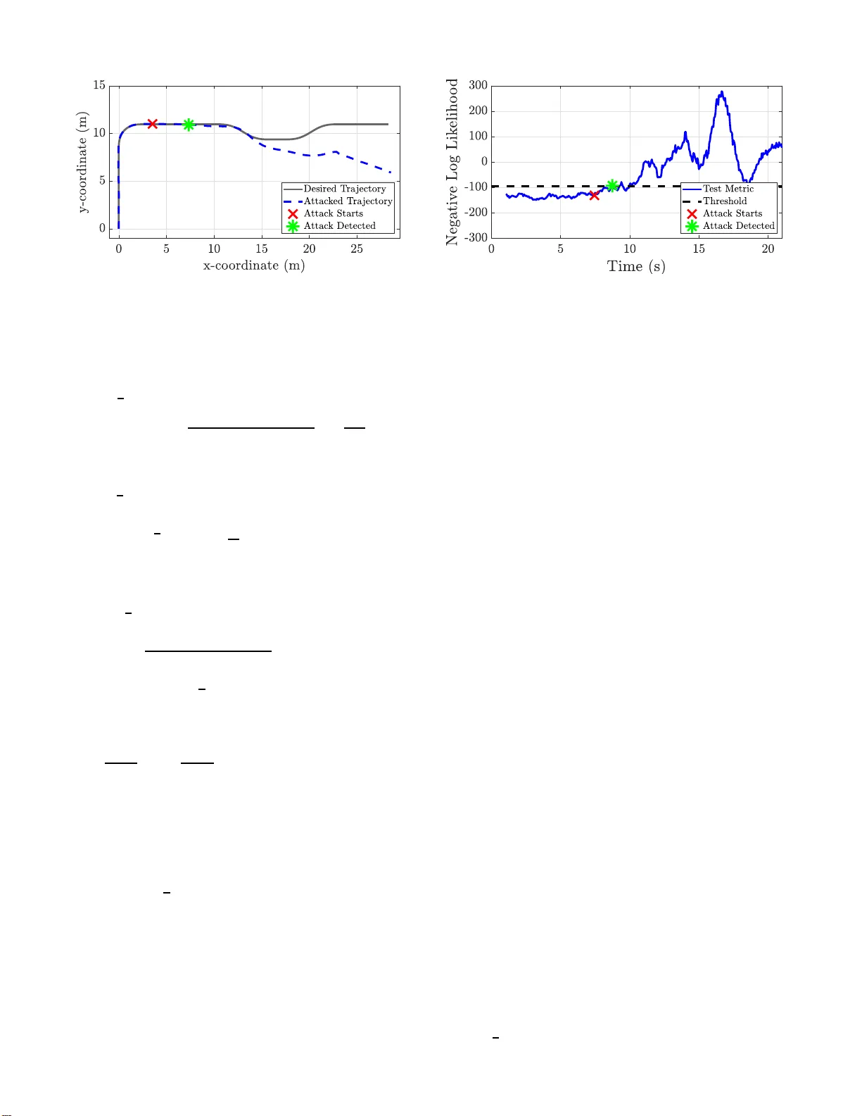
1 Detecti ng Generaliz ed Replay Attacks via T ime-V arying Dyn amic W aterma rking Matthew Porter , Pedro Hespanhol, Anil Aswani, Matthew Joh n son-Roberso n, and Ra m V asudevan Abstract —Cyber -physical systems (CPS) often rely on external communication f or supervisory control or sensing. Unfo rtunately , these communications render the system vulnerable to cyber - attacks. Attacks that alter messages, such as replay attacks that record measur ement signals and then play them back to the system, ca n cause de vasta ting effects. Dynamic W atermarking methods, which inject a private excitation into control i n puts to secure resulting measurement signals, hav e b egun addressing the challenges of detecting these attacks, but hav e been restricted to lin ear time in variant (L TI) systems. Though L TI models ar e sufﬁcient f or some appl i cations, other CPS, su ch as autonomous vehicles, require more complex models. Th is paper dev elops a linear time-varying (L TV) extension to p re vious Dynamic W atermarking methods b y designi n g a matrix normalization factor to accomm odate th e temporal changes in the system. Implementable tests are prov ided with considerations for rea l- world systems. The proposed method is then shown to be able to detect generalized replay attacks both in theory and in simulation using a L TV vehicle model. I . I N T RO D U C T I O N Cyber-physical systems (CPS) comb ine both networked computin g an d sensing resources with physical contro l sys- tems in an effort to increase efﬁciency , manag e complexity , or provide con venience. Whether it is industrial contr ol ap- plications or smart devices, CPS require secu r e networked commun ications to op erate safely and correctly . Malicious attacks on suc h systems ca n cause dev astating resu lts [1] – [4]. CPS are often protected b y traditional cyber secur ity tools, but th ese methods are insufﬁcient due to the addition of networked p h ysical infra stru cture. [5], [6] . A gr owing body of work has started to address these challeng es by developing new detection a lgorithms, analy zing po tentially stealthy attack models, a n d ﬁnding ways of re d ucing the ef fect of attacks. One particular detectio n m ethod, Dyn amic W atermark ing, has been shown to d etect various attack models while making few a s- sumptions about system stru cture. De sp ite these developments, detection algorithm s, including Dynamic W atermarkin g, have only f ocused o n CPS that can be m odeled as linear time in variant (L TI) systems. While L TI models ca n be su fﬁcient for steady state or slo w movin g applications, many emerging CPS This work was s upported by a grant from Ford Motor Company via the Ford-UM Allianc e under award N022977 and by UC Berke ley Center for Long-T erm Cybersecuri ty . M. Porter and R. V asudev an are with the Department of Mechani cal Engineeri ng, Unive rsity of Michigan, Ann Arbor , MI 48103 USA (e- mail: m atthepo@umich.edu ; ramv@umich.ed u). A. Aswani and P . Hespanhol are with the Depart ment of Industrial E ngineer - ing and Operat ions Research, Univ ersity of California Berkele y , Berk ele y , CA 94720 USA (e-mail: aaswa ni@berk ele y .edu; pedrohespa nhol@berk ele y . edu). M. Johnson-Roberson is with the Department of Nav al Architec ture, Uni- versi ty of Michi gan, Ann Arbor , MI 48103 USA (e-mail : matt jr@umich.edu) . such as autonomo us vehicles requir e mod els tha t chan g e over time. T his paper develops methods to ac c ommod a te such CPS by extending Dynamic W atermar king to linear time-varying (L TV) systems. A. Attac k Mod els Attacks are divided in to three categories: denia l o f service (DOS) a tta cks , where the contro l or measure m ent signal is stopped, direct atta cks , w h ere the plant, actu ators or sensors are phy sically attacked, an d decep tio n attacks , where th e control o r measurem ent signal are altered. [7]. DOS attacks can be detrimen tal, but are tr i vial to detect if they stop all comm unication. Fur th ermore, wh e n only a po rtion of commun ication is stoppe d, their effects can be minimized using g raceful degrad ation [ 8]. T he result of direct attacks often causes anomalies in the m e asurement signal a n d can therefor e b e detected b y methods u sed to d etect deception attacks. Consequentially , this work fo cuses on the detection of d eception attack s. A variety of d e ception attacks have bee n propo sed. The simplest deceptio n a ttac k s add noise u sing arbitrary or rand o m strategies [9 ]. On the other hand, bias injection attacks, the attacker injects a constant bias into th e sy stem [10], while routing attack s send measur e ment signals throu gh a linear transform [11 ] . Oth er deception attacks attem pt to deco u ple the system such that the m e a surements are una lter ed while ce rtain states of the system ar e attacked [1 2]. For instance, zero- dynamics attacks take advantage of un -observable states or remove the effects of their attacks in the r e sulting measureme nt signal [10 ], an d replay attacks in volve a n attacker replaying recorde d m easurements while possibly alter ing control as well [10]. The amount of k n owledge of the system dynamics an d detection schem e alo n g with the capability of th e attacker to alter certain signals necessary to c arry out th ese attacks varies greatly . While random, bia s injection , rou ting, an d rep la y attacks do not requir e any knowledge of the un derlying system dynamics, d e c oupling and zero-dyn a m ics attack require a lm ost full knowledge. This k nowledge can be difﬁcult to obtain for non-in sider attackers but it is no t impo ssible [ 13], [14]. Nonetheless, this work fo cuses on a genera lization of a r eplay attack d ue to th e simplicity of implem entation and because it has alread y b een applied d uring real-world attacks [ 1]. Further- more, we co nsider attacks that only alter measuremen t sign a ls, since many o f the systems we care ab out use local con trollers while op erating using externally received me a su rements. 2 B. Attac k Detection Algo rithms The measur ement r esidu al , deﬁned as th e difference be- tween the measu r ement and the expected m easurement, is used by most detection schemes. For each detector, a me tr ic based on the me a surement residu al is generate d . If at any time the metric exceed s a user-deﬁned th reshold, the detector raises an alarm. Genera lly , these m etrics can b e sep arated into two categories: tho se that only observe the system , called pa ssive methods , and those that alter the system while observin g, called active metho ds . While passive metho ds do not degrade control perform ance, active methods accep t a small amount of perfor mance degradation in exchange for the ab ility to detec t more complex attacks [15]–[17 ]. These categories can b e further subd i vided into stateless m etrics, which on ly consider the cu r rent measuremen t re sidual, and stateful metrics, which rely o n pr evious m easurement r esiduals as well. 1) P assive Meth o ds: The χ 2 detector’ s metric is th e inner produ ct of the normalized m e a surement residual, which fol- lows a χ 2 distribution. Due to its simplicity , the χ 2 detector has been studied in several works [18]–[ 21]. Thoug h the χ 2 is widely used, it is a stateless detector . T wo stateful a lter natives are the cum ulativ e sum (CUSUM) detector and the multi- variate expo nentially weigh ted moving average (MEWMA) detector . When compa r ing these statefu l detecto rs to the χ 2 detector, it has been sh own that the statefu l de tec tors can often pr ovide strong er guarantee s on d etection while the χ 2 detector boasts both simpler im plementation a n d generally takes less tim e to detect attacks [22], [23 ] . While pa ssive detectors can detect rand o m attacks, th ey are unable to detect more sophisticated attacks su ch as replay attacks. In a ddition, they have only be e n developed for L TI systems. 2) Active Method s: Most a cti ve metho ds fall into o ne o f two categories: moving tar get defen se , which change system parameters to keep attackers fr om ob taining the current con- ﬁguration , and watermarking-b ased methods , which encryp t measuremen t signals with a watermar k that is added to the control in p ut. The con cept of m ovin g ta rget defe nses is a topic of con- tinued interest for the ﬁeld of cyber security and includes random izing the or der of code execution an d physical memory storage location s [24]. In CPS, moving target defense can take the form o f switching between red undan t measurem ents [25]– [29], alterin g co n trol strategy [25], [ 2 9], or b y ch a nging plant dyna mics [ 25]–[ 2 7], [30]– [33]. Switching m e asurement signals works we ll whe n an attacker is only hackin g a few mea surements, but other wise p e rforms similar to passive methods. Altering the control strategy is argua b ly similar to watermarking- based method s and can a llow fo r detection of most attack m odels except zero- dynamics attacks. While som e methods alter the p h ysical plan t d ynamics directly [25]– [27], others a ppend th e plant dyn amics with an au xiliary system with po ssibly mor e complex dynam ics [3 0]–[3 3]. Despite the consideratio n of mo re complex dyn a m ics for the auxiliary systems, moving target defen se has only been applied to systems that have L TI dyna m ics. Altho ugh co mplex d ynamics cause the behavior o f the test metric to change in time, methods for selecting a time- varying thresho ld inv olve hand tuning. Alter ing p la n t dyn amics can allow f or d e te c tion of all attack mod els, but the meth od makes certain assumption s about the system. Note, for the auxiliary systems it is assumed that the plant has secu re knowledge o f its o wn state, wh ich does no t account for vulnerable networked sensors. Also, when an auxiliary system is not used, it is assumed tha t the p lant dynamics ar e ch angeable . The introduction o f a watermark was ﬁrst prop osed as a way of makin g the χ 2 detector r o bust to r eplay attacks [ 3 4] and other mor e a d vanced attacks [35 ]. Here, the watermark takes the form o f indepen dent iden tically d istributed (I ID) Gaussian noise that is added to the contro l inpu t. Robustness to re p lay attacks is then ach iev ed by p roperly selectin g th e watermark covariance, while the χ 2 detector itself rem ains unchan ged. Dynamic W aterma r king u ses a m etric that relies on bo th th e covariance o f the residuals and the co rrelation b etween the residuals and the watermar k . The c ov ariance o f th e watermark is allowed to be an arbitr a ry sy mmetric f ull ran k matrix [3 6]– [40]. In th ese works, the me tr ic uses the measurement residuals contained in a tempora lly sliding window . Guar antees o f detection are the n mad e as the wind ow size tends to inﬁn ity . Extensions to a limited sub set of nonlin ear system s have been implemented [38 ] , [41], but otherwise Dynam ic W atermark ing has b een limited to L TI systems. T hough th e ad dition o f the watermark causes a degra d ation in system perfor m ance, the degradation can be m inimized [42], [43 ] . Other work has considered allowing th e watermar k signal to b e au to-corre lated [44] or to have distributions th at are not Gau ssian [4 5], [46]. Furthermo re, other forms of watermarks include intentio n al package dro ps [4 7], [48] , u sin g parameterized tran sforms on measurements [11], [ 49], [ 50], and B-sp lines added to feed fo rward inpu ts [51]. Thoug h Dyn amic W ate r marking is unable to d etect zero -dynam ic s attacks, it does not requir e the assumption of chan geable plant dy n amics or lo cally secure knowledge of p lant state. This p a per focuses o n Dynamic W atermar king as d escribed in Hespanhol et al. [37] due to its ability to b e app lied to a wide range of L TI systems including both fu lly and partially observable systems. C. Con tributions The contr ibutions of this p aper are thr eefold. First, the tests used in He sp anhol et al. [37] are extended to L TV systems. This is done using a carefu lly desig n ed matrix no rmalization factor to accom modate the tempo ral ch anges in the system. These tests are then proven to de tec t gener alized r eplay attacks. Secon d, a model is developed for time-varying ge n - eralized rep lay attacks. Thir d , L TV Dy namic W a te r marking is applied to a simulated system to provide p r oof of conce p t. The rem ainder of this pap er is organized as follows. Section I-D intro duces notation. Section I I revie ws the metho d s in Hes- panho l et al. [37] to motivate the need for L TV Dynamic W a- termarkin g. Asym ptotic guara n tees a n d implemen table tests for L TV Dyn amic W aterm a rking are provided in Sections III and IV respectively . Simu la ted results are presented in Section V. The app endix covers statistical bac kgrou n d for the pr oofs in th is paper in addition to a few larger e quations that have been removed from pro ofs to improve readability . 3 D. Notation This sectio n breiﬂy introduc es the no tation used in this paper . The 2-no r m o f a vector x is denoted k x k . Similarly , the 2-no rm of a matrix X is den oted k X k . The tr ace of a matrix X is deno ted tr ( X ) . Zero matrices of dim ension i × j are den oted 0 i × j , and in the c ase that i = j , the notation is simpliﬁed to 0 i . Identity ma tr ices of dim ension i are d enoted I i . The W ishart distribution with scale matrix Σ and i degrees of freedom is d enoted W (Σ , i ) [52, Sectio n 7.2]. The mul- ti variate Gaussian d istribution with mean µ and covariance Σ is denoted N ( µ, Σ) . The ch i-squared distribution with i degrees of freedom is d e noted χ 2 ( i ) . The expe c ta tio n of a random variable a is deno ted E [ a ] . The probab ility o f an event E is denoted P ( E ) . Given a sequence of random variables { a i } ∞ i =1 , conv ergence in pr obability is denoted p-lim i →∞ a i and alm ost sure convergence is deno ted as-lim i →∞ a i [53, Deﬁnition 7.2.1] . I I . I N S P I R A T I O N F O R LT V W AT E R M A R K I N G This section d escribes the in spiration for L T V dynamic wa- termarkin g by summ arizing the m e thod describ ed in Hespan- hol et al. [37 ] fo r L TI systems. Consider an L TI system with state x n , measur ement y n , process n oise w n , measurement noise z n , watermark e n , additive attack v n , and stabilizing feedback that uses the ob served state ˆ x x n +1 = Ax n + B K ˆ x n + B e n + w n (1) ˆ x n +1 = ( A + B K + LC ) ˆ x n + B e n − Ly n (2) y n = C x n + z n + v n (3) where x n , ˆ x n , w n ∈ R p , e n ∈ R q , y n , z n , v n ∈ R r , and x 0 = 0 p × 1 . The p rocess no ise w n , measuremen t noise z n , and watermar k e n are mu tually indepen dent an d take the form w n ∼ N (0 p × 1 , Σ w ) , z n ∼ N (0 r × 1 , Σ z ) , and e n ∼ N (0 q × 1 , Σ e ) . While the pro cess and me asurement noise a re unknown to the contr oller , the watermark signal is g e n erated by the co ntroller and is known. The following assumption is made on th e co ntroller, observer, and watermark d esign. Assumption II.1. Assume k A + B K k < 1 , k A + LC k < 1 , and Σ e is full rank. The measuremen t residual for this system takes the fo rm C ˆ x n − y n . When an attack is not present, the distribution of the mea surement residuals converge to a zero mean Gaussian distribution with covariance Σ wher e Σ = lim n →∞ E [( C ˆ x n − y n )( C ˆ x n − y n ) ⊺ ] . (4) Note, f o r a L TV system , the limit in (4) may n ot exist. Next, conside r a generaliza tion o f a replay attack satisfying v n = α ( C x n + z n ) + C ξ n + ζ n (5) ξ n +1 = ( A + B K ) ξ n + ω n (6) where α ∈ R is called the a ttack scalin g factor , the false state ξ n ∈ R p has p rocess noise ω n ∈ R p and measureme nt noise ζ n ∈ R r that take the fo rm ω n ∼ N (0 p × 1 , Σ ω ) and ζ n ∼ N (0 r × 1 , Σ ζ ) , an d are mutually in depend ent with each other and with w n and z n . Note, when Σ ω and Σ ζ are selected such that the covariance of the measure m ent residual is una lter ed and the attack scalin g p arameter is − 1 , this model describes a rep lay attack. While attackers may have the ab ility to star t and stop attacks at will, attack s that are on ly pr e sen t for ﬁnite time are n ot guar a nteed to b e detected. T herefor e, when considerin g asymptotic guar antees o f detection, the assumption of persistence is made . T o formally describe these persistent attack s, con sid e r the following deﬁnition. Deﬁnition II.2 . Th e asympto tic attack power is de ﬁned as as-lim i →∞ 1 i P i − 1 n =0 v ⊺ n v n . (7) Under this deﬁnition, an attack with no n-zero asymptotic power is d eemed to be persistent. The asymptotic claims of L TI dyn amic watermark ing take the fo rm o f the following theorem . Theorem II.3. [37, Theor em 1] Consider an attacked L TI system satisfying (1 ) - (3) , an a ttack mo del satisfying (5) - (6) , and Σ satisfying (4) . Let k ′ = min { k ≥ 0 | C ( A + B K ) k B 6 = 0 r × q } be ﬁ nite. If as-lim i →∞ 1 i P i − 1 n =0 ( C ˆ x n − y n )( C ˆ x n − y n ) ⊺ = Σ (8) and as-lim i →∞ 1 i P i − 1 n =0 ( C ˆ x n − y n ) e ⊺ n − k ′ − 1 = 0 r × q , (9) then th e asympto tic attack power is 0. The delay of the waterma r k b y k ′ in (9 ) ensures th at the effect o f the watermark is present in th e measur ement signal. Note, the contrap o siti ve of Theorem II.3 states that for attacks with n on-zer o asymp totic power , (8) and (9 ) ca n not both be satisﬁed. Ther e f ore, consider ing the LHS o f (8 ) and (9), generalized r eplay attack s of non-zer o asymp totic power ar e guaran tee d to b e detected in inﬁnite time. T o m ake th ese tests implementable in real time, a statistical test is derived using a sliding w in dow o f ﬁxed size. At eac h step, the co mbined partial sums in (8)-(9) ta ke the form S n = P n + ℓ i = n +1  ( C ˆ x i − y i ) e i − k ′ − 1   ( C ˆ x i − y i ) ⊺ e ⊺ i − k ′ − 1  . (10) Under the assumption of n o attack, S n conv erges asympto ti- cally to the W ishart distribution with scale matrix S =  Σ 0 r × q 0 q × r Σ e  (11) and ℓ degrees of fre e dom as ℓ → ∞ . Furtherm ore, f or a generalized r e play attack o f non-ze r o asymptotic power , Theorem II .3 gives us that the scale matrix for S n is n o long er S , since either ( 8) or (9) is not satisﬁed. Given the sampled matrix S n , the te st then u ses th e negativ e log likeliho o d of th e scale m atrix L ( S n ) = ( m + q + 1 − ℓ ) log ( | S n | ) + tr  S − 1 S n  . (12) Negati ve log likelihood values th at exceed a u ser deﬁned threshold, signal an attack. 4 For L TV systems, the limits in (8 )-(9) may not exist. Furthermo re, the sampled matrices S n may no lo nger be approx imated a s a Wis hart d istribution since the vectors u sed to c reate it in (10) ar e not necessarily id entically d istributed. T o a c c ommod a te th ese changes in distribution, it is necessary to develop a new method . I I I . LT V D Y NA M I C W AT E R M A R K I N G This section derives th e limit-b ased formulation of Dy namic W atermar king for a discrete- tim e L TV system. First, the L TV d ynamics, necessary assump tions, and the r esulting limit based tests are deﬁned . Subsequ ently , Sectio n III- A p rovides intermediate r esults to p rove these claims. Consider an L TV sy stem with state x n , mea su rement y n , process noise w n , measuremen t no ise z n , watermark e n , additive attack v n , and stabilizing feedb a c k that uses the observed state ˆ x x n +1 = A n x n + B n K n ˆ x n + B n e n + w n (13) y n = C n x n + z n + v n (14) where x n , ˆ x n , w n ∈ R p , e n ∈ R q , y n , z n , v n ∈ R r , and x 0 = 0 p × 1 . The p rocess no ise w n , measuremen t noise z n , and watermar k e n are mu tually indepen dent an d take the form w n ∼ N (0 p × 1 , Σ w, n ) , z n ∼ N (0 r × 1 , Σ z ,n ) , an d e n ∼ N (0 q × 1 , Σ e ) . While th e process and measu r ement noise are unknown to the contro ller , the watermar k sig nal is generated by the contro ller and is known. For simplicity , deﬁne ¯ A n = ( A n + B n K n ) and ¯ A ( n,m ) = ¯ A n · · · ¯ A m for n ≥ m and ¯ A ( n,n +1) = I p . W e make th e f ollowing assumption. Assumption III.1. The covariances Σ e , Σ w, n , a nd Σ z ,n , of the rand o m variables used in (1 3) - (14) , ar e full rank. Further- mor e, there exists po sitive con sta nts η w , η z , η ¯ A , η B , η C ∈ R such that k Σ w, n k < η w , k Σ z ,n k < η z , k ¯ A n k < η ¯ A < 1 , k B n k < η B , and k C n k < η C , for a ll n ∈ N . The assumption of bound ed full ra n k covariances for the process an d measurement n oise are satisﬁed for mo st systems by mo deling error and sensor no ise. Furtherm ore, the inpu t and output matrices are often constrained to be ﬁnite by sensor an d actuator limits. Sinc e the watermar k an d controller ar e user deﬁned, the remain d er o f th e assumptions can be satisﬁed so long as th e system is controllable. W e make the fo llowing assumption. Assumption III.2. lim i →∞ 1 i P i − 1 n =0 C n B n − 1 6 = 0 r × q . (15) Here, (15) guarante e s an asymptotic c o rrelation betwe e n th e measuremen t signal y n and the watermark signal e n − 1 , which has been delayed by a single time step. This ensure s that the watermark has a persistent measur able e ffect o n the measuremen t signal, wh ich can then be used for validation purpo ses. This is similar to assuming k ′ is equal to 0 fo r the L TI case. The observer an d the correspo nding ob server erro r , deﬁne d as δ n = ˆ x n − x n , satisfy ˆ x n +1 = ( ¯ A n + L n C n ) ˆ x n + B n e n − L n y n (16) δ n +1 = ( A n + L n C n ) δ n − w n − L n ( z n + v n ) , (17) where ˆ x 0 = δ 0 = 0 p × 1 . For simplicity , d eﬁne A n = ( A n + L n C n ) and A ( n,m ) = A n · · · A m for n ≥ m a nd A ( n,n +1) = I p . Furth ermore, let ¯ δ n +1 = A n ¯ δ n − w n − L n z n (18) ˆ δ n +1 = A n ˆ δ n − L n v n (19) where ¯ δ 0 = ˆ δ 0 = 0 p × 1 . Note that δ n = ¯ δ n + ˆ δ n and that when v n = 0 r × 1 , ∀ n we have that ˆ δ n = 0 p × 1 , ∀ n . Here ¯ δ n can be though t of as the por tio n o f the observer error that results from the orig inal noise o f the system, while ˆ δ n is the con tribution of th e attac k to the observer er r or . Next, co n sider the expected value Σ δ,n = E [ ¯ δ n ¯ δ ⊺ n ] = E [ δ n δ ⊺ n | v n = 0 r × 1 , ∀ n ] , which can be written as Σ δ,n = P n i =0 A ( n − 1 ,n − i +1) (Σ w, n − i + + L n − i Σ z ,n − i L ⊺ n − i ) A ⊺ ( n − 1 ,n − i +1) . (20) The ma trix n o rmalization facto r is then deﬁned as V n = ( C n Σ δ,n C ⊺ n + Σ z ,n ) − 1 / 2 , (21) which exists sin c e Σ z ,n is full r ank. For an L TI system, the matrix V n = Σ − 1 / 2 where Σ is as deﬁned in (4). For the L TV system, the matrix normalizatio n factor can be thoug ht of as a time-varying n ormalization fo r the measurem ent residu al. Next, we make th e following assumptio n about the o bserver . Assumption III.3. There exists p ositive constants η A , η L , η δ , η V ∈ R such that k A n k < η A < 1 , k L n k < η L , k Σ δ,n k < η δ , and k V n k < η V , for all n ∈ N . If the system in ( 13)-(14) is observable, then the user deﬁned controller can satisfy the assum ption on A n . Previous assump- tions imply the assumption s on L n , Σ δ,n , and V n are satisﬁed, but the bound s here ar e used to simplify notation . Next, we alter the attack deﬁned in (5)-(6 ) to cre ate a tim e- varying equiv alent. Consider an attack v n that satisﬁes v n = α ( C n x n + z n ) + C n ξ n + ζ n (22) ξ n +1 = ¯ A n ξ n + ω n , (23) where α ∈ R is called the attack scaling fa ctor , the false state ξ n ∈ R p has p rocess noise ω n ∈ R p and me asurement noise ζ n ∈ R r that take the form ω n ∼ N (0 p × 1 , Σ ω ,n ) and ζ n ∼ N (0 r × 1 , Σ ζ ,n ) an d are mutua lly indepen dent with each other an d with w n and z n . Similar to the L TI case, whe n Σ ω ,n and Σ ζ ,n are selected properly and the attack scaling p arameter is − 1 , this mod el describes a replay attack. Th e results of such an attack can have dev astating r esults as shown in Figure 1 . While a n attacker cou ld choose to allow the noise to have unbou nded c ov ariance, the resulting attack would be tr i vial to detect. Ther efore, we make the fo llowing assumption abo u t the attack m odel. Assumption III.4. When th er e is an attack, v n follows the dynamics (2 2) - (23) with the attack scaling factor remaining constant. Furth e rmor e, there e xists po sitive constants η ω , η η ∈ R su ch that k Σ ω ,n k < η ω , k Σ ζ ,n k < η ζ , for all n ∈ N . 5 T o make asymptotic guaran tees of detectio n , we also assume the persistence of attack s using the following deﬁnition . Deﬁnition III.5. The asympto tic attack power is deﬁned as p-lim i →∞ 1 i P i − 1 n =0 v ⊺ n v n . (24) Similar to prior research in Dynamic W aterma rking, we ﬁrst deﬁne th e asymptotic tests. Theorem III.6. Co nsider an attacked LTV system sa tisfying the dy n amics in ( 1 3) - (19) . Let V n be as deﬁn ed in (21 ) . If v n = 0 r × 1 , for a ll n ∈ N , th en p-lim i →∞ 1 i P i − 1 n =0 V n ( C n ˆ x n − y n ) e ⊺ n − 1 = 0 r × q (C1) and p-lim i →∞ 1 i P i − 1 n =0 V n ( C n ˆ x n − y n )( C n ˆ x n − y n ) ⊺ V ⊺ n = I r . (C2) Furthermore , if the a ttack follows the dyn amics in (22) - (23) and h a s non -zer o asymptotic power as deﬁn e d in Deﬁnition III.5, th en (C1) and (C2) cann o t both be satisﬁed. From Theorem I II.6, the LHS of (C1) and (C2) can b e used to guarantee detection of generalized replay attacks with non -zero asymp totic power in inﬁnite time. Note, ( C1 ), (C2), and (24) u se limits in probability as opp osed to the almost sure limits u sed in their L TI counter parts. This change removes the gu arantee of detectio n via the asym p totic tests for certain pathological examples of attack s, but both form s of con vergence provide th e sam e motiv ation fo r th e statistical tests in Section IV. Given an arbitr ary real n umber ǫ , alm o st sure conv ergence states that with probability 1 the sequ ence will remain a distance of less than ǫ from the limit after a ﬁnite numb e r o f steps while conver gence in p robability states that the prob a bility that an element of the sequenc e is within a distance of ǫ from th e limit co n verges to 1 as yo u continu e along the seq u ence. Since the statistical tests use a sliding window to consider only a ﬁnite number of steps at a time, both forms of con vergence say that as the wind ow size grows the sequenc e of sample averages become mor e likely to be closer to the limit when no attack is pr esent. As a resu lt, th e test b e comes mo re sensitive. A. Intermediate Results T o prove Th eorem I II.6, several intermediate results must ﬁrst be provided . First, we consider the asymptotic limit (C1) and show th at it implies α is equ al to 0. This allows us to assume that α is equal to 0 for the remainder of th e intermediate r esults. Theorem III.7. Co nsider an attacked LTV system sa tisfying (13) - (19) and the attack mod el satisfying (22) - (23) . Let V n be as deﬁned in (2 1) . ( C1) holds if an d on ly if the attack scaling factor α is eq ual to 0 . Pr o of. (Theorem III.7) Assume that α is equal to 0. Rearr ang- ing th e L HS o f (C1) using (14), (17), an d (2 2) r e su lts in p-lim i →∞ 1 i P i − 1 n =0 V n ( C n ˆ x n − y n ) e ⊺ n − 1 = = p -lim i →∞ 1 i P i − 1 n =0 V n ( C n δ n − z n − C n ξ n − ζ n ) e ⊺ n − 1 . (25) Corollary A.5 says that to sh ow that the RHS of (2 5) conver ges in pro bability to 0 r × q , it is sufﬁcient to show that each term in the sum converges in proba b ility to 0 r × q . Note that p-lim i →∞ 1 i P i − 1 n =0 V n ( C n δ n − C n ξ n ) e ⊺ n − 1 = 0 r × q (26) by Corollary A. 7 since e n − 1 is independ ent id entically dis- tributed with bou nded covariance, and V n ( C n δ n − C n ξ n ) is a bound ed lin ear transform o f a ran dom vector that satisﬁes the necessary auto corr elation bound as a r esult of Theor em A.9. Similarly , p-lim i →∞ 1 i P i − 1 n =0 V n ( − z n − ζ n ) e ⊺ n − 1 = 0 r × q (27) by Cor ollary A . 7 since z n , ζ n , and e n − 1 are mutually in - depend ent iden tically distributed w ith bou nded covariances. Therefo re α = 0 implies (C1) h olds. Now assume that (C1) h o lds. Rearrang in g (C1) using ( 14), (17), an d (2 2) results in p-lim i →∞ 1 i P i − 1 n =0 V n ( C n ˆ x n − y n ) e ⊺ n − 1 = = p -lim i →∞ 1 i P i − 1 n =0 V n ( C n δ n − (1 + α ) z n + − αC n x n − C n ξ n − ζ n ) e ⊺ n − 1 . (28) Now since (27) holds by the same argumen t as bef ore, we can use Theorem A.4 to cancel these terms resulting in p-lim i →∞ 1 i P i − 1 n =0 V n ( C n ˆ x n − y n ) e ⊺ n − 1 = = p -lim i →∞ 1 i P i − 1 n =0 V n ( C n δ n − αC n x n ) e T n − 1 . (29) Expand ing x n in (29) b y on e step using (13) then results in p-lim i →∞ 1 i P i − 1 n =0 V n ( C n ˆ x n − y n ) e ⊺ n − 1 = = p-lim i →∞ 1 i P i − 1 n =0 V n ( C n δ n − αC n ( A n − 1 x n − 1 + + B n − 1 K n − 1 ˆ x n − 1 + B n − 1 e n − 1 + w n − 1 )) e ⊺ n − 1 . (30) Using Coro llary A.7 we have that p-lim i →∞ 1 i P i − 1 n =0 − αV n C n B n − 1 ( e n − 1 e ⊺ n − 1 − Σ e ) = 0 q × r . (31) Therefo re by The o rem A.4 we have p-lim i →∞ 1 i P i − 1 n =0 V n ( C n ˆ x n − y n ) e ⊺ n − 1 = = p-lim i →∞ 1 i P i − 1 n =0 V n ( C n δ n − αC n ( A n − 1 x n − 1 + + B n − 1 K n − 1 ˆ x n − 1 + w n − 1 )) e ⊺ n − 1 + αV n C n B n − 1 Σ e . (32) Note, th at all eleme nts of V n ( C n δ n − αC n ( A n − 1 x n − 1 + + B n − 1 K n − 1 ˆ x n − 1 + w n − 1 )) e ⊺ n − 1 (33) are distributed symmetrically abo ut 0 for all n ∈ N . Con sider an elem ent of (32 ) for which the correspon ding element in 1 i P i − 1 n =0 V n C n B n − 1 Σ e (34) 6 does n ot converge. For eac h i , the prob ability that the ma tr ix element in (32) is farther away from 0 than the correspond ing element in (34) is a t least 0 . 5 . The r efore the elemen t can not conv erge in pro bability to 0 comple tin g the p roof.  Assuming α is equal to 0, we show that ( C2) is eq uiv alent to anoth er condition th at is o nly dep endent on the attack v n and its contr ibution to the ob server erro r ˆ δ n . No te, ˆ δ n is not a com putable quan tity given the av ailable knowledge o f th e system, but the provided intermediate co ndition is an amen able surrogate to (C2). Theorem III.8. Co nsider an attacked LTV system sa tisfying (13) - (19) a n d an atta ck mod e l satisfying (2 2) - (23) . Let V n be as deﬁned in (21) . Assume the attack scaling factor α is equal to 0. ( C2 ) hold s if and only if p-lim i →∞ 1 i P i − 1 n =0 V n ( C n ˆ δ n − v n )( C n ˆ δ n − v n ) ⊺ V ⊺ n = 0 r . (35) Pr o of. (Theorem III.8 ) Exp anding (C2) using (14) and (1 7)- (19) g ives us p-lim i →∞ 1 i P i − 1 n =0 V n ( C n ˆ x n − y n )( C n ˆ x n − y n ) ⊺ V ⊺ n = = p -lim i →∞ 1 i P i − 1 n =0 V n ( C n ¯ δ n − z n )( C n ¯ δ n − z n ) ⊺ V ⊺ n + + V n ( C n ¯ δ n − z n )( C n ˆ δ n − v n ) ⊺ V ⊺ n + + V n ( C n ˆ δ n − v n )( C n ¯ δ n − z n ) ⊺ V ⊺ n + + V n ( C n ˆ δ n − v n )( C n ˆ δ n − v n ) ⊺ V ⊺ n . (36) By Co rollary A.7 an d Theor em A.9, p-lim i →∞ 1 i P i − 1 n =0 V n ( C n ¯ δ n − z n )( C n ¯ δ n − z n ) ⊺ V ⊺ n = I r (37) and p-lim i →∞ 1 i P i − 1 n =0 V n ( C n ¯ δ n − z n )( C n ˆ δ − v n ) ⊺ V ⊺ n = 0 r (38) since, by the deﬁnition of V n in (2 1 ), the expectation for each summand in (37) is I r , and V n ( C n ¯ δ n − z n ) is unco r related with V n ( C n ˆ δ − v n ) . First, assume th at (C2) holds. By Theorem A. 4 , it follows fr om (3 6 )-(38) that ( 35) must hold. Next, assume that (35) hold s. By Co r ollary A.5, it f ollows from (3 6)-(38) th at (C2) ho lds.  Since the attack v n , under the assump tion that α is equal to 0, is only d ependen t on th e rando m vector s ξ n and ζ n , we now provide sufﬁcient and n ecessary con ditions on these r andom vectors for the asymptotic attack power to be 0. Similar to Theorem I II.8, these rand om vectors are not co mputable by the controller, but the resulting conditions can be u sed to con nect (C2) to th e asymp totic attack power . Theorem III.9. Co nsider an attacked LTV system sa tisfying (13) - (19) and a n attack mod el satisfying (22) - (23) . Assume that th e attack sca ling factor α is equal to 0. The asymptotic attack power as deﬁned in (2 4 ) is 0 if and o nly if p-lim i →∞ 1 i P i − 1 n =0 ζ n ζ ⊺ n = 0 (39) and p-lim i →∞ 1 i P i − 1 n =0 C n ξ n ξ ⊺ n C ⊺ n = 0 r . (40) Pr o of. (Th eorem II I.9) Assume th a t α = 0 . U sin g Lem ma A.10 we have that the asympto tic a ttac k power is 0 if and only if p-lim i →∞ 1 i P i − 1 n =0 v n v ⊺ n = 0 r . (41) Expand ing th e LHS of (41) using (22)-(23 ) we get an equva- lent con dition. p-lim i →∞ 1 i P i − 1 n =0 C n ξ n ξ ⊺ n C ⊺ n + + C n ξ n ζ ⊺ n + ( C n ξ n ζ ⊺ n ) ⊺ + ζ n ζ ⊺ n = 0 r (42) Since ξ n and ζ n are uncor related, f rom Theorem A.9 and Corollary A.7 we have p-lim i →∞ 1 i P i − 1 n =0 C n ξ n ζ ⊺ n = 0 r . (43) First, assume th at (39 ) and ( 40) hold. By Corollary A.5 we have that (4 2) must ho ld since, whe n separated , the limit f or each term converges to 0 r . Next, assume that (4 2) h o lds. By Theorem A.4 we can rewrite (42 ) as p-lim i →∞ 1 i P i − 1 n =0 ζ n ζ ⊺ n + C n ξ n ξ ⊺ n C ⊺ n = 0 r , (44) since (43) h olds. No te, bo th term s are positive-semideﬁnite matrices. T herefor e , f or an arbitr a ry ǫ > 0 we have that P     1 i P i − 1 n =0 ζ n ζ ⊺ n    > ǫ  ≤ ≤ P     1 i P i − 1 n =0 ζ n ζ ⊺ n + C n ξ n ξ ⊺ n C ⊺ n    > ǫ  (45) Furthermo re, (44) imp lies lim i →∞ P     1 i P i − 1 n =0 ζ n ζ ⊺ n + C n ξ n ξ ⊺ n C ⊺ n    > ǫ  = 0 r , ∀ ǫ > 0 (46) Then, by (45 ) an d (46 ) lim i →∞ P     1 i P i − 1 n =0 ζ n ζ ⊺ n    > ǫ  = 0 r , ∀ ǫ > 0 . (47) Therefo re, (39) must hold. Applying Theorem A.4 to (44) using ( 39) imp lies (4 0) must also h old.  Next, we start to complete the conn ection between (C2) an d zero asymptotic attack power b y proving (35) implies (39). Furthermo re, we prove a related result that makes it simpler to pr ove th at ( 35) implies (4 0 ). Theorem III.10. Consider an attacked L TV system satisfying (13) - (19) and an a ttack mod el satisfying (2 2) - (23) . Let V n be as deﬁned in (21) . Assume the attack scaling factor α is equ al to 0. I f (35) holds, then ( 39) ho ld s as well and p-lim i →∞ 1 i P i − 1 n =0 ( C n ˆ δ n − C n ξ n )( C n ˆ δ n − C n ξ n ) ⊺ = 0 r . (48 ) Pr o of. (Th eorem III. 10) Assume th at (3 5 ) h olds. Exp anding the LHS of (35 ) using (22 ) we get p-lim i →∞ 1 i P i − 1 n =0 V n ( C n ˆ δ n − C n ξ n )( C n ˆ δ n − C n ξ n ) ⊺ V ⊺ n + 7 + V n ( C n ˆ δ n − C n ξ n ) ζ ⊺ n V ⊺ n + ( V n ( C n ˆ δ n − C n ξ n ) ζ ⊺ n V ⊺ n ) ⊺ + + V n ζ n ζ ⊺ n V ⊺ n = 0 r . (49) Using Coro llary A. 7 and Theo rem A.9 we have p-lim i →∞ 1 i P i − 1 n =0 V n ( C n ˆ δ n − C n ξ n ) ζ ⊺ n V ⊺ n = 0 r . (50) Therefo re, by ap p lying Th e orem A.4 to (49) we have p-lim i →∞ 1 i P i − 1 n =0 V n ( C n ˆ δ n − C n ξ n )( C n ˆ δ n − C n ξ n ) ⊺ V ⊺ n + + V n ζ n ζ ⊺ n V ⊺ n = 0 r . (51) Note, b oth term s are positi ve-semideﬁnite matrices. Using the same method u sed on (44 ), we then have p-lim i →∞ 1 i P i − 1 n =0 V n ζ n ζ ⊺ n V ⊺ n = 0 r (52) and p-lim i →∞ 1 i P i − 1 n =0 V n ( C n ˆ δ n − C n ξ n )( C n ˆ δ n − C n ξ n ) ⊺ V ⊺ n = 0 r . (53) W e co m plete the pr oof using Lemma A.1 1 but we must ﬁrst provide lower b ound on the eig en values o f V ⊺ n V n . Let λ n denote the smallest eignen value o f V ⊺ n V n , then λ n is lower bound ed since λ n = 1 k ( V ⊺ n V n ) − 1 k = 1 k C n Σ δ,n C ⊺ n + Σ z ,n k ≥ ≥ 1 η 2 C η δ + η z > 0 . (54) If we assume that (39 ) does not hold then applying Lemma A.11 co ntradicts (5 2). Th erefore (39 ) must ho ld . Similarly , assuming that (48) does n ot hold would resu lt in a contradictio n with ( 5 3). The r efore (48) must also hold.  Next we prove that (35) im p lies (40) to complete the relation between (C2) an d the asympto tic attack power . Theorem III.11. Consider an attacked LTV system satisfying (13) - (19) a n d an atta ck mod e l satisfying (2 2) - (23) . Let V n be as deﬁned in (21) . Assume the attack scaling factor α is equal to 0. I f (35) holds th en (4 0) h olds as well. T o prove Theo rem III .11, we instead p rove the con trapos- iti ve statemen t by a ssuming that (40) does not ho ld, pr oving that (48) do es not h old eith e r , then using Th eorem III .10 we complete the p roof. T o do th is, we split the sum mation in (40) accord ing to the following lem ma. This split allows us to disregard the cross terms on th e L HS of (48 ) and sh ows that the remaining term s do no t conver ge in p robability to 0 r . Lemma III.12. Co nsider an attacked LTV system satisfying (13) - (19) a n d an atta ck mod e l satisfying (2 2) - (23) . Let V n be as deﬁned in (21) . Assume the attack scaling factor α is equal to 0. I f (40 ) do es not ho ld then ther e exists m ∈ N fo r which p-lim i →∞ 1 i P i − 1 n =0  C n P m n j =1 ¯ A ( n − 1 ,n − j +1) ω n − j  × ×  C n P m n j =1 ¯ A ( n − 1 ,n − j +1) ω n − j  ⊺ 6 = 0 r . (55) wher e m n = min { n , m } . F urthermor e, ther e e xists a n m ′ ∈ N such that m ′ ≤ m a n d p-lim i →∞ 1 i P i − 1 n =0 C n ¯ A ( n − 1 ,n − j +1) ω n − j × × ω ⊺ n − j ¯ A ⊺ ( n − 1 ,n − j +1) C ⊺ n 6 = 0 r (56) for j = m ′ but not fo r j < m ′ . Pr o of. (Le mma III.1 2) First, we prove the existence of m . Assume that (40 ) does n o t hold. Exp a n ding the LHS of (40) using ( 23) results in p-lim i →∞ 1 i P i − 1 n =0  P n j =1 C n ¯ A ( n − 1 ,n − j +1) ω n − j  × ×  P n j =1 C n ¯ A ( n − 1 ,n − j +1) ω n − j  ⊺ 6 = 0 r . (57) Then, usin g Lemm a A.10 we have that p-lim i →∞ 1 i P i − 1 n =0    P n j =1 C n ¯ A ( n − 1 ,n − j +1) ω n − j    2 6 = 0 . (58) Since (4 0) d oes no t hold there exists ǫ, τ > 0 such tha t P  1 i P i − 1 n =0    P n j =1 C n ¯ A ( n − 1 ,n − j +1) ω n − j    2 > ǫ  > τ (59) for inﬁn itely many i . W e prove that there exists an m such that fo r each i that (59 ) holds we have P  1 i P i − 1 n =0    P m n j =1 C n ¯ A ( n − 1 ,n − j +1) ω n − j    2 > ǫ 6  > τ 4 (60) which is equiv alent to (55) as a result of Lemma A.10. T o make statements on the truncated sum, we start by ﬁnd in g the relationship between the prob ability in th e LHS o f (59) and the pro bability in the LHS of (6 0). For each i such that (59 ) holds, we app ly triang le ineq uality to g et τ < P  1 i P i − 1 n =0     P m n j =1 C n ¯ A ( n − 1 ,n − j +1) ω n − j    + +    P n j = m n +1 C n ¯ A ( n − 1 ,n − j +1) ω n − j     2 > ǫ  . (61) Further expan ding and applying Theorem A.1 r e sult in τ < P  1 i P i − 1 n =0    P m n j =1 C n ¯ A ( n − 1 ,n − j +1) ω n − j    2 > ǫ 3  + + P  2 i P i − 1 n =0    P m n j =1 C n ¯ A ( n − 1 ,n − j +1) ω n − j    × ×    P n j = m n +1 C n ¯ A ( n − 1 ,n − j +1) ω n − j    > ǫ 3  + + P  1 i P i − 1 n =0    P n j = m n +1 C n ¯ A ( n − 1 ,n − j +1) ω n − j    2 > ǫ 3  . (62) Focusing on the center term in the RHS of (62), we can write P 2 i P i − 1 n =0    P m n j =1 C n ¯ A ( n − 1 ,n − j +1) ω n − j    × ×    P n j = m n +1 C n ¯ A ( n − 1 ,n − j +1) ω n − j    > ǫ 3 ! ≤ 8 ≤ P r 2 i P i − 1 n =0    P m n j =1 C n ¯ A ( n − 1 ,n − j +1) ω n − j    2 × × r 2 i P i − 1 n =0    P n j = m n +1 C n ¯ A ( n − 1 ,n − j +1) ω n − j    2 > ǫ 3 ! ≤ ≤ P  2 i P i − 1 n =0    P m n j =1 C n ¯ A ( n − 1 ,n − j +1) ω n − j    2 > ǫ 3  + + P  2 i P i − 1 n =0    P n j = m n +1 C n ¯ A ( n − 1 ,n − j +1) ω n − j    2 > ǫ 3  , (63) where the ﬁrst inequality c omes from a pplying the Cauchy Schwarz I n equality and the second inequality co mes f rom applying Theorem A.2 . Then since P  1 i P i − 1 n =0    P m n j =1 C n ¯ A ( n − 1 ,n − j +1) ω n − j    2 > ǫ 3  ≤ ≤ P  2 i P i − 1 n =0    P m n j =1 C n ¯ A ( n − 1 ,n − j +1) ω n − j    2 > ǫ 3  (64) and P  1 i P i − 1 n =0    P n j = m n +1 C n ¯ A ( n − 1 ,n − j +1) ω n − j    2 > ǫ 3  ≤ ≤ P  2 i P i − 1 n =0    P n j = m n +1 C n ¯ A ( n − 1 ,n − j +1) ω n − j    2 > ǫ 3  , (65) we can co mbine (62 ) with (63)-(6 5) to obtain τ < 2 P  1 i P i − 1 n =0    P m n j =1 C n ¯ A ( n − 1 ,n − j +1) ω n − j    2 > ǫ 6  + + 2 P  1 i P i − 1 n =0    P n j = m n +1 C n ¯ A ( n − 1 ,n − j +1) ω n − j    2 > ǫ 6  . (66) If we can up per bo und the secon d term in the RHS or (66 ) by τ 2 the ﬁrst term must b e lower b o unded by τ 2 completing the p roof. T o p rovide this bound we make use o f Markov’ s Inequa lity . T o this end, we ﬁr st boun d the expec ta tio n E  1 i P i − 1 n =0    P n j = m n +1 C n ¯ A ( n − 1 ,n − j +1) ω n − j    2  = = E 1 i P i − 1 n =0 P n j = m n +1  C n ¯ A ( n − 1 ,n − j +1) ω n − j  ⊺ × ×  C n ¯ A ( n − 1 ,n − j +1) ω n − j  ! ≤ ≤ E  1 i P i − 1 n =0 P ∞ j = m +1  C n + j ¯ A ( n + j − 1 ,n +1) ω n  ⊺ × ×  C n + j ¯ A ( n + j − 1 ,n +1) ω n   ≤ 1 i P i − 1 n =0 P ∞ j = m +1 pη 2 C η 2( j − 1) A 1 η 2 ω = pη 2 C η 2 m A 1 η 2 ω 1 − η 2 A 1 , (67) where th e the ﬁrst equality com es from expan ding th e norm and ignoring uncorr elated terms, the ﬁrst inequa lity comes from rearrang ing the summation and allowing the second summation to go to inﬁnity , the second inequality comes from distributing the expectation and upper bound ing each elemen t, and the ﬁnal equality comes from e valuating the sum mations. Since η A 1 < 1 , we can choo se m sufﬁciently large such that pη 2 C η 2 m A 1 η 2 ω 1 − η 2 A 1 < τ ǫ 24 . (68) Using Mar kov’ s inequality [54 , Equation 5.31] we h av e that P  1 i P i − 1 n =0    P n j = m n +1 C n ¯ A ( n − 1 ,n − j +1) ω n − j    2 > ǫ 6  ≤ ≤ 6 pη 2 C η 2 m A 1 η 2 ω (1 − η 2 A 1 ) ǫ < τ 4 (69) which c ompletes the pro of for the existence of m . Next, we prove the existence of m ′ . Con sider the expansion of ( 5 5) p-lim i →∞ 1 i P i − 1 n =0 C n P m n j =1 P m n k =1 ¯ A ( n − 1 ,n − j +1) ω n − j × × ω ⊺ n − k ¯ A ⊺ ( n − 1 ,n − k +1) C ⊺ n 6 = 0 . (70) Considering th e summ ands where j 6 = k we have that p-lim i →∞ 1 i P i − 1 n =0 C n ¯ A ( n − 1 ,n − j +1) ω n − j × × ω ⊺ n − k ¯ A ⊺ ( n − 1 ,n − k +1) C ⊺ n = 0 (71) by Theo rem A.6 since ω n is in depende nt an d the dynamics are bo unded an d stable. If we furth e r assume that ther e does not exist an m ′ for which (56) ho lds then by The orem A.1 we h av e that (55) do es n ot hold which is a contradictio n. Therefo re, the set of integers less that or equal to m for which (56 ) hold s, is a non- empty ﬁnite set. The smallest element of this set then satisﬁes the conditio ns for m ′ .  Now returning to prove the Theore m. Pr o of. (Th eorem III.1 1) WLOG, in this proof , we allow sum - mations to re f erence variables with negati ve index by assuming these values to be 0 r to ease notation. Assume th a t (35) holds but ( 40) does not. Since (40) do es not hold, m ′ be chosen such that it satisﬁes the d escription in L emma III.12. Fro m Theorem III .10 we have tha t (35) implies (48). Ex p anding the LHS of (4 8) using (23) gives us p-lim i →∞ 1 i P i − 1 n =0 ( C n ˆ δ n − C n ξ n )( C n ˆ δ n − C n ξ n ) ⊺ = = p -lim i →∞ 1 i P i − 1 n =0  C n  ˆ δ n − P n j =1 ¯ A ( n − 1 ,n − j +1) ω n − j  × ×  ˆ δ n − P n k =1 ¯ A ( n − 1 ,n − k +1) ω n − k  ⊺ C ⊺ n  = 0 r . ( 72) By sep arating the ind ex m ′ we can write p-lim i →∞ 1 i P i − 1 n =0 ( C n ˆ δ n − C n ξ n )( C n ˆ δ n − C n ξ n ) ⊺ = = p -lim i →∞ 1 i P i − 1 n =0 C n ˆ δ n − P 1 ≤ j ≤ n j 6 = m ′ ¯ A ( n − 1 ,n − j +1) ω n − j ! × × ˆ δ n − P 0 ≤ k ≤ n k 6 = m ′ ¯ A ( n − 1 ,n − k +1) ω n − k ! ⊺ C ⊺ n + − C n ˆ δ n − P 1 ≤ j ≤ n j 6 = m ′ ¯ A ( n − 1 ,n − j +1) ω n − j ! × × ω ⊺ n − m ′ ¯ A ⊺ ( n − 1 ,n − m ′ +1) C ⊺ n − C n ¯ A ( n − 1 ,n − m ′ +1) ω n − m ′ × 9 × ˆ δ n − P 0 ≤ k ≤ n k 6 = m ′ ¯ A ( n − 1 ,n − k +1) ω n − k ! ⊺ C ⊺ n + + C n ¯ A ( n − 1 ,n − m ′ +1) ω n − m ′ × × ω ⊺ n − m ′ ¯ A ⊺ ( n − 1 ,n − m ′ +1) C ⊺ n = 0 r . (73) For now suppo se that p-lim i →∞ 1 i P i − 1 n =0 − C n ˆ δ n − P 1 ≤ j ≤ n j 6 = m ′ ¯ A ( n − 1 ,n − j +1) ω n − j ! × × ω ⊺ n − m ′ ¯ A ⊺ ( n − 1 ,n − m ′ +1) C ⊺ n = 0 r . (74) Then by T heorem A. 4 we have that p-lim i →∞ 1 i P i − 1 n =0 ( C n ˆ δ n − C n ξ n )( C n ˆ δ n − C n ξ n ) ⊺ = = p -lim i →∞ 1 i P i − 1 n =0 C n ˆ δ n − P 1 ≤ j ≤ n j 6 = m ′ ¯ A ( n − 1 ,n − j +1) ω n − j ! × × ˆ δ n − P 0 ≤ k ≤ n k 6 = m ′ ¯ A ( n − 1 ,n − k +1) ω n − k ! ⊺ C ⊺ n + + C n ¯ A ( n − 1 ,n − m ′ +1) ω n − m ′ × × ω ⊺ n − m ′ ¯ A ⊺ ( n − 1 ,n − m ′ +1) C ⊺ n = 0 r . (75) Furthermo re, by o ur ch oice of m ′ we have th at p-lim i →∞ 1 i P i − 1 n =0 C n ¯ A ( n − 1 ,n − m ′ +1) ω n − m ′ × × ω ⊺ n − m ′ ¯ A ⊺ ( n − 1 ,n − m ′ +1) C ⊺ n 6 = 0 r , (76) and sin ce th e terms are all positive-semideﬁnite ma trices P    1 i P i − 1 n =0 C n ¯ A ( n − 1 ,n − m ′ +1) ω n − m ′ × × ω ⊺ n − k ¯ A ⊺ ( n − 1 ,n − k +1) C ⊺ n   > ǫ  ≤ ≤ P      1 i P i − 1 n =0 C n ˆ δ n − P 1 ≤ j ≤ n j 6 = m ′ ¯ A ( n − 1 ,n − j +1) ω n − j ! × × ˆ δ n − P 0 ≤ k ≤ n k 6 = m ′ ¯ A ( n − 1 ,n − k +1) ω n − k ! ⊺ C ⊺ n + + C n ¯ A ( n − 1 ,n − m ′ +1) ω n − m ′ × × ω ⊺ n − m ′ ¯ A ⊺ ( n − 1 ,n − m ′ +1) C ⊺ n      > ǫ ! . (77) This implies that (73 ) cannot hold which contradic ts (35). Therefo re (40 ) m ust h o ld since o therwise there exists an m ′ satisfying L emma A. 11. T o complete the pro o f, we now show that (74) indeed ho lds. by Cor ollary A.5 th is is equivalent to p roving p-lim i →∞ 1 i P i − 1 n =0 C n P 1 ≤ j ≤ n j 6 = m ′ ¯ A ( n − 1 ,n − j +1) ω n − j × × ω ⊺ n − m ′ ¯ A ⊺ ( n − 1 ,n − m ′ +1) C ⊺ n = 0 r (78) and p-lim i →∞ 1 i P i − 1 n =0 − C n ˆ δ n ω ⊺ n − m ′ ¯ A ⊺ ( n − 1 ,n − m ′ +1) C ⊺ n = 0 r . (79) Note, (78) ho lds b y Corollary A.7 since all ω n are mutu ally indepen d ent, k C n ¯ A ( n − 1 ,n − m ′ +1) k ≤ k C n k < η C , and the auto-cor relation is bo unded by (156) in th e app endix. Fur - thermor e , expa nding the LHS o f (79) u sing (1 9) gives us p-lim i →∞ 1 i P i − 1 n =0 − C n ˆ δ n ω ⊺ n − m ′ ¯ A ⊺ ( n − 1 ,n − m ′ +1) C ⊺ n = = p -lim i →∞ 1 i P i − 1 n =0 C n  P n − 1 j =0 A ( n − 1 ,j +1) L j ζ j + P n k =1 A ( n − 1 ,n − k +1) L n − k C n − k × × P n ℓ = k +1 ¯ A ( n − k − 1 ,n − ℓ +1) ω n − ℓ  × × ω ⊺ n − m ′ ¯ A ⊺ ( n − 1 ,n − m ′ +1) C ⊺ n = 0 r . (80) T o prove that (79) ho lds, we use Corollar y A. 5 o n (80 ) and show that each term conv erges to 0 r . Note, b y Theore m A.6, p-lim i →∞ 1 i P i − 1 n =0 C n  P n − 1 j =0 A ( n − 1 ,j +1) L j ζ j  × × ω ⊺ n − m ′ ¯ A ⊺ ( n − 1 ,n − m ′ +1) C ⊺ n = 0 r , (81) since k C n ¯ A ( n − 1 ,n − m ′ +1) k ≤ η C , ζ n and ω n are mu tually indepen d ent, and the au to-corr e la tio n is b ounded by (1 57) in the appendix . Furthermore, c onsidering the portion o f ˆ δ n not depend ent on ω n − m ′ , by T h eorem A.6 , p-lim i →∞ 1 i P i − 1 n =0 C n P n j =1 A ( n − 1 ,n − j +1) L n − j C n − j × × P n k = j +1 k 6 = m ′ ¯ A ( n − j − 1 ,n − k +1) ω n − k × × ω ⊺ n − m ′ ¯ A ⊺ ( n − 1 ,n − m ′ +1) C ⊺ n = 0 r , (82) since ω n are indep endent, k C n ¯ A ( n − 1 ,n − m ′ +1) k ≤ η C , an d the auto-cor relation is boun ded by (158 ) in the a p pendix . Now if p-lim i →∞ 1 i P i − 1 n =0 C n P m ′ − 1 j =1 A ( n − 1 ,n − j +1) L n − j C n − j × × ¯ A ( n − j − 1 ,n − m ′ +1) ω n − m ′ × × ω ⊺ n − m ′ ¯ A ⊺ n − 1 ,n − k +1 C ⊺ n = 0 r , (83) we have completed the proof. T o show this, we show that th e trace o f the matr ix converges to 0 for each value of j . p-lim i →∞ 1 i P i − 1 n =0  ω ⊺ n − m ′ ¯ A ⊺ ( n − 1 ,n − m ′ +1) C ⊺ n × × C n A ( n − 1 ,n − j +1) L n − j C n − j × × ¯ A ( n − j − 1 ,n − m ′ +1) ω n − m ′  ≤ ≤ p -lim i →∞  1 i P i − 1 n =0   C n ¯ A ( n − 1 ,n − m ′ +1) ω n − m ′   2  1 / 2 × ×  1 i P i − 1 n =0   C n A ( n − 1 ,n − j +1) L n − j × × C n − j ¯ A ( n − j − 1 ,n − m ′ +1) ω n − m ′   2  1 / 2 (84) where th e inequ a lity follow from the Cauchy Schwarz Inequal- ity . Let ǫ, τ > 0 b e c h osen ar bitrarily . N o te that by Markov’ s Inequa lity P  1 i P i − 1 n =0   C n ¯ A ( n − 1 ,n − m ′ +1) ω n − m ′   2 ≥ ≥ 2 η 2 C η 2( m ′ − 1) A 1 η ω 1 − τ  ≤ ≤ (1 − τ ) E h 1 i P i − 1 n =0 k C n ¯ A ( n − 1 ,n − m ′ +1) ω n − m ′ k 2 i 2 η 2 C η 2( m ′ − 1) A 1 η ω ≤ ≤ (1 − τ ) η 2 C η 2( m ′ − 1) A 1 η ω 2 η 2 C η 2( m ′ − 1) A 1 η ω = 1 − τ 2 . (85) 10 Fig. 1. Desired and attack ed trajec tory of an L TV car model showin g atta ck start and dete ction (Left); Corresponding L TV Dynamic W atermarking test metric sho wing attac k s tart and detection (right) Furthermo re by o ur choice of m ′ , we have th at there exists an N such that i > N implies P  1 i P i − 1 n =0   C n − j ¯ A ( n − j − 1 ,n − m ′ +1) ω n − m ′   2 ≤ ≤ ǫ 2 2 η 4 C η 2( m ′ − 1) A 1 η 2( j − 1) A 2 η 2 L η ω  ≥ τ +1 2 . (86) Finally , applyin g Theorem A.3 P  1 i P i − 1 n =0   C n ¯ A ( n − 1 ,n − m ′ +1) ω n − m ′   2  1 / 2 × ×  1 i P i − 1 n =0   C n A ( n − 1 ,n − j +1) L n − j × × C n − j ¯ A ( n − j − 1 ,n − m ′ +1) ω n − m ′   2  1 / 2 ≤ ǫ  ≥ ≥ P  1 i P i − 1 n =0   C n − j ¯ A ( n − j − 1 ,n − m ′ +1) ω n − m ′   2 ≤ ǫ 2 2 η 4 C η 2( m ′ − 1) A 1 η 2( j − 1) A 2 η 2 L η ω  + +  1 − P  1 i P i − 1 n =0   C n ¯ A ( n − 1 ,n − m ′ +1) × × ω n − m ′   2 ≥ 2 η 2 C η 2 A 1 η ω  − 1 ≥ (87) ≥ τ + 1 2 + 1 − 1 − τ 2 − 1 = τ . (88) Therefo re (83) m ust hold .  Having proven se veral intermediate results, we are now able to formally prove Th eorem II I.6. Pr o of. (Theorem II I.6) When n o attack is present, (C1) holds using T heorem I II.7 since α is equal to 0. Furtherm ore, (C2) holds sin c e δ = δ . Now assume that an attack of non- z e ro asymptotic power is pr esent and con sider the following cases. Case 1 ( α 6 = 0 ): Usin g Theorem III .7, (C1) do es not hold. Case 2 ( α = 0 ): Note, (C2) implies zero asympto tic attack power as follows. (C2) ⇐ ⇒ Thm. III.8 (35) = ⇒ Thm. III.10 (39) = ⇒ Thm. III.11 (40) ⇐ ⇒ Thm. III.9  zero a symptotic attack p ower  Under our assumption of non -zero asymptotic power , the contrapo siti ve imp lies tha t (C2) does not hold.  I V . I M P L E M E N TA B L E S TA T I S T I C A L T E S T S While Section III provides a necessary backgro und f or L TV Dynamic W aterm arking, inﬁnite limits are n ot well suited f or real tim e attack detection . This section der i ves a statistical test using a slidin g wind ow app roach. Let ψ n =  V n ( C n ˆ x n − y n ) e n − 1  (89) and Q n = [ ψ n − ℓ . . . ψ n ][ ψ n − ℓ . . . ψ n ] ⊺ . (90) where ℓ + 1 is the wind ow size, ℓ ∈ N , and ℓ ≥ q + r − 1 . No te, ψ n is asympto tically u ncorre late d and id entically distributed such th at ψ n ∼ N (0 q + r × 1 , S ) , fo r n = 1 , 2 , 3 , · · · where S =  I r 0 r × q 0 q × r Σ e  . (91 ) Therefo re, un der th e assumption of no attack, the distribution of Q n approa c h es a W isha rt distribution with ℓ + 1 degrees of freedom and scale matrix S a s ℓ g oes to inﬁnity . Further more, for a gen e ralized replay attack with n on-zero asymptotic power , Theo rem III.6 proves that the scale matrix for Q n is no longer S since e ither (C1) or (C2) is not satisﬁed. Th e Wis hart distribution c an then be u sed to deﬁne a statistical test using the negative log likelihood of the scale matrix S given the sampled matrix Q n : L ( Q n ) = ( q + r − ℓ ) log( | Q n | ) + tr ( S − 1 Q n ) . (92) In theo ry , if the pro cess and m e asurement noise c ov ariances Σ w, n and Σ z ,n are kn own, V n can be calcu lated using (20)- (21). In practice, th ese covariances are difﬁcult to estimate which c an lead to err or in th e estima te of V n . T o reduce this error, V n can be directly estimated using a n ensemb le av erage of i r ealizations such that V n ≈  1 i P i j =1 ( C n ˆ x ( j ) n − y ( j ) n )( C n ˆ x ( j ) n − y ( j ) n ) ⊺  − 1 / 2 (93) 11 Fig. 2. Simulat ed L TI and L TV Dynamic W atermarking test metrics for L TV car model under no attack where the supe r script ( j ) is th e index of th e realizatio n. Th is approx imation is approp riate since by the weak law of large number s we h av e that when no attac k is pr esent p-lim i →∞ 1 i P i j =1 ( C n ˆ x ( j ) n − y ( j ) n )( C n ˆ x ( j ) n − y ( j ) n ) ⊺ = = C n Σ δ,n C ⊺ n + Σ z ,n (94) and V n is de ﬁned as in (21). V . S I M U L A T E D R E S U LT S T o provide pro of of co ncept, we use a simpliﬁed car mod el       x y ψ v ˙ ψ       =       v cos( ψ ) v sin( ψ ) ˙ ψ a ¨ ψ       , (95) where the car has grou nd p lane coor dinates ( x, y ) , heading ψ , forward velocity v , and angular velocity ˙ ψ . Using the desired trajectory shown in Figu re 1, (95) is linearized and discretized u sing a step size of 0.0 5 and zero order hold on the curren t state and input. The con troller and observer for the r esulting L TV system are fo und using a line a r q uadratic regulator ( LQR) to stabilize the system. Furthermo re, the process an d measure ment noise covariances are chosen suc h that they scale linearly with the velocity . T o compar e L TI a nd L TV Dynamic W atermarkin g, a time in variant matrix normalization factor is calcu lated using the av erage o f th e r e sidual c ov ariance, while the time-varying matrix nor malization factor is calcu lated using (20 )-(21). For both cases, we run 10 0 simulations with a window size of 20 and calcula te the test metr ic a nd th e average test metric as shown in Figure 2. Note, while the L TV Dy namic W ater- marking metric remain s consistent over the entire simulation, the L TI counterp art has a rep eatable time-varying pattern . Using the u n-attacked data, a thre sh old fo r the L TV case is found such that the rate at wh ic h false alarm s occur do e s not exceed once p er ev ery 50 seconds of run time . Next consider an attack mod el satisfying (13 )-(19), with α equ al to − 1 a n d the measureme n t and p rocess noise matching that of the tr u e system. The results of this attack on the system, and the ability of L TV Dyn amic W atermarkin g to q uickly detect it, are shown in Figu r e 1. V I . C O N C L U S I O N This paper d eriv es Dyna m ic W ate r marking for L TV sys- tems, and provid e s asymptotic guarantee s in addition to im- plementab le tests. A L TV genera lized replay attack is deﬁne d and sh own to be de tectable by the Dy namic W atermark ing method d ev eloped in this work. Furth ermore, a vehicle mo d el with L TV Dynam ic W atermarkin g is simulated to p rovide proof of c oncept of the implemen table tests. Using these simulations, the L TV Dy namic W atermark ing is compare d to its L TI counterp a r t and is shown to provide a mo re con sistent test me tric. R E F E R E N C E S [1] R. L angner , “Stuxnet : Dissect ing a cyberwa rfare weapon, ” IEEE Security & P r ivacy , vol. 9, no. 3, pp. 49–51, May 2011. [2] M. Abrams and J. W ei ss, “Malici ous control system cyber security attack case s tudy - Maroochy water service s, australia, ” MITRE , 2008. [3] R. M. Lee, M. J. Assante, and T . Conway , “German steel mill cybe r attac k, ” Industrial Contr ol Systems , vol. 30, p. 62, 2014. [4] ——, “ Analysis of the cyber attac k on the ukrainian po wer grid, ” Electric ity Information Sharing and Analysis Center (E -ISAC) , 2016. [5] H. Sandber g, S. Amin, and K. H. Johansson, “Cybe rphysical secu rity in netw orked contro l systems: An introduction to the issue, ” IEEE Contr ol Systems Magazine , vol. 35, no. 1, pp. 20–23, 2015. [6] A. A. C ´ a rdenas, S. Amin, and S. Sastry , “Research challen ges for the security of control systems, ” in Pr oceed ings of the 3rd Confer ence on Hot T opics in Security , ser . HOTSEC’08. Berkele y , CA, USA: USENIX Associati on, 2008, pp. 1–6. [7] A. A. C ´ ardenas, S. Amin, and S. Sastry , “Secure control : T o ward s sur- vi v able cybe r-physic al systems, ” in The 28th Internatio nal Confer enc e on Distribute d Computing Systems W orkshops , June 2008, pp. 495–500. [8] S. Amin, A. A. C ´ a rdenas, and S. Sastry , “Safe and secure network ed control systems under denial-o f-service attacks, ” in International W ork- shop on Hybrid Systems: Computation and Contr ol . Berlin, Heidelbe rg: Springer , 2009, pp. 31–45. [9] Y . Liu, P . Ning, and M. K. Reiter , “False data injectio n attac ks against state estimation in ele ctric power grids, ” AC M T ransact ions on Informa- tion and System Securit y (TISSEC) , vol. 14, no. 1, pp. 13:1–13 :33, Jun. 2011. [10] A. T eixeira , D. P ´ ere z, H. Sandbe rg, and K. H. Johansson, “ Attack models and scenar ios for netwo rked control systems, ” in Pr oceedi ngs of the 1st Internati onal Confere nce on High Conﬁdence Network ed Systems , s er . HiCoNS ’12. Ne w Y ork, NY , USA: ACM, 2012, pp. 55–64. [11] R. M. Ferrari and A. M. T eixeira , “Detec tion and isolat ion of routin g attac ks through sensor wat ermarking, ” in 2017 Annual American Contr ol Confer enc e (ACC) , May 2017, pp. 5436–5442. [12] R. S. Smith, “ A decouple d feedback structure for cov ertly approp riating netw orked control systems, ” IF AC P r ocee dings V olumes , vol. 44, no. 1, pp. 90 – 95, 2011. [13] Y . Y uan and Y . Mo, “Security in cybe r-physic al systems: Controlle r design against kno wn-plain text attack, ” in 54th IEEE Conferen ce on Decision and Contr ol (CDC) , Dec 2015, pp. 5814–5819. [14] D. Umsonst, E. Nek ouei, A. M. T eix eira , and H. Sandberg, “On the conﬁdentiali ty of linear anomaly detecto r states, ” in 2019 Annual American Contr ol Confer enc e (ACC) , July 2019, pp. 397–403. [15] M. Porter , A. Joshi, P . Hespanhol, R. V asudev an, and A. Aswani, “Simulat ion and real-w orld e v aluati on of att ack detec tion schemes, ” in 2019 A nnual A merican Contro l Confer enc e (ACC) , July 2019, pp. 551– 558. [16] S. W eerakk ody , O. Ozel, P . Grifﬁoen, and B. Sinopoli, “ Activ e detection for exposing intelli gent att acks in control systems, ” in 2017 IEEE Confer enc e on Contr ol T echnolo gy and Application s (CCTA) , Aug 2017, pp. 1306–1312. 12 [17] S. W eerakkody , B. Sinopoli, S. Kar, and A. Datta, “Information ﬂ ow for security in control systems, ” in 55th IEEE Confer ence on Decision and Contr ol (CDC) , Dec 2016, pp. 5065–5072. [18] Y . Mo, E. Garone, A. Casavol a, and B. Sinopoli, “F alse data inje ction attac ks against state estimation in wireless sensor networks, ” in 49th IEEE Confer ence on Decision and Contr ol (CDC) , Dec 2010, pp. 5967– 5972. [19] Y . Mo and B. Sinopoli , “Inte grity attac ks on cyber -physic al systems, ” in Proc eedings of the 1st Internati onal Confer ence on High Conﬁdence Network ed Systems , ser . HiCoNS ’12. New Y ork, NY , USA: ACM, 2012, pp. 47–54. [20] C. Kwon, W . L iu, and I. Hwang, “Security analysis for c yber-ph ysical systems against stealthy decep tion attacks, ” in 2013 Annual American Contr ol Conferen ce (ACC) , June 2013, pp. 3344–3349. [21] N. Hashemi and J. Ruths, “Gene ralize d chi-squared detec tor for lti systems with non-gaussian noise, ” in 2019 Annual American Contr ol Confer enc e (ACC) , July 2019, pp. 404–410. [22] C. Murgui a and J. Ruths, “CUSUM and Chi-squared Atta ck Detec tion of Compromised Sensors, ” in 2016 IEEE Confe re nce on Contr ol Appli- cations (CCA) , Sep 2016, pp. 474–480. [23] D. Umsonst and H. Sandber g, “Anomaly Detector Metrics for Sensor Data Attacks in Control Systems, ” in 2018 Annual American Contr ol Confer enc e (ACC) , June 2018, pp. 153–158. [24] S. Jajodia, A. K. Ghosh, V . Swarup , C. W ang, and X. S. W ang, Mov- ing targ et defense: creat ing asymmetric uncertainty for cyber threat s . Springer Science & Business Media, 2011, vol. 54. [25] A. M. T eixeira, I. Shames, H. Sandber g, and K. H. Johansson, “Re veal- ing s teal thy attack s in contr ol systems, ” in 2012 50th Annual A llerton Confer enc e on Communi cation, Contr ol, and Computi ng (Allerton) , Oct 2012, pp. 1806–1813. [26] M. A. Rahman, E. Al-Shaer , and R. B. Bobba, “Movi ng tar get defense for hardening the s ecurit y of the power system state estimation, ” in Pr oceedi ngs of the Fir st ACM W orkshop on Moving T arget Defe nse , ser . MTD ’14. Ne w Y ork, NY , USA: A CM, 2014, pp. 59–68. [27] J. T ian, R. T an, X. Guan, and T . Liu, “Hidden moving target defense in smart grids, ” in Pr ocee dings of the 2nd W orkshop on Cyber-Phy sical Securit y and Resilience in Smart Grids , ser . CPSR-SG’17. New Y ork, NY , USA: A CM, 2017, pp. 21–26. [28] J. Giraldo, A. A. C ´ ardenas, and R. G. Sanfe lice, “ A moving targe t defense to detect stealthy attac ks in cyber-ph ysical systems, ” in 2019 Annual American Contr ol Confer enc e (ACC) , July 2019, pp. 391–396. [29] A. Kanell opoulos and K. V amvoudaki s, “Swit ching for unpredic tabili ty: A proact i ve defense control approach, ” in 2019 Annual A merican Contr ol Conferen ce (ACC) , July 2019, pp. 4338–4343. [30] S. W eerakko dy and B. Sinopoli , “Detecting inte grity attac ks on control systems using a moving target approach, ” in 54th IEE E Confer ence on Decision and Contr ol (CDC) , Dec 2015, pp. 5820–5826. [31] C. Schelle nberge r and P . Zhang, “Dete ction of cov ert attacks on cyber - physical systems by ext ending the s ystem dynamics with an auxiliary system, ” in 56th IEEE Confere nce on Decisi on and Contr ol (CDC) , D ec 2017, pp. 1374–1379. [32] M. Ghade ri, K. Gheitasi , and W . L ucia, “ A nove l control archite cture for the detection of false data injection attacks in network ed control systems, ” in 2019 Annual American Contr ol Conferen ce (ACC) , July 2019, pp. 139–144. [33] P . Grif ﬁoen, S. W eerakk ody , and B. Sinopol i, “ An optimal design of a moving targe t defense for attack detec tion in control systems, ” in 2019 Annual A merican Contr ol Confere nce (ACC) , July 2019, pp. 4527–4534. [34] Y . Mo and B. Sinopol i, “Secure control again st replay attac ks, ” in 2009 47th Annual Allerton Confer ence on Communicati on, Contr ol, and Computing (Allerton ) , Sept 2009, pp. 911–918. [35] S. W ee rakkod y , Y . Mo, and B. Sinopoli, “Detecting integri ty attacks on control systems using robust physical watermarkin g, ” in 53rd IEEE Confer enc e on Deci sion and Contr ol (CDC) , Dec 2014, pp. 3757–3764. [36] B. Satchidananda n and P . R. Kumar , “Dynamic W atermarking: Acti ve Defense of Networke d Cyber -Physical Systems, ” Pr oceedi ngs of the IEEE , vol. 105, no. 2, pp. 219–240, 2017. [37] P . Hespanhol , M. Porter , R. V asude v an, and A. Aswa ni, “Dynamic wate rmarking for general lti systems, ” in 56th IE EE Confer enc e on Decision and Contr ol (CDC) , Dec 2017, pp. 1834–1839. [38] B. Satchidananda n and P . Kumar , “Defending cyber -physica l s ystems from sensor attacks, ” in International Confere nce on Communication Systems and Networks . Springe r , 2017, pp. 150–176. [39] P . Hespanhol, M. Porter , R. V asude v an, and A. Aswani, “Statist ical wate rmarking for networ ked control systems, ” in 2018 Annual American Contr ol Conferen ce (ACC) , June 2018, pp. 5467–5472. [40] J. Rubio-He rnan, L. De Cicco, and J. Garcia-Alfa ro, “Event-t riggered wate rmarking control to handle cybe r-physic al integrity attacks, ” in Nor dic Confer ence on Secur e IT Systems . Springer , 2016, pp. 3–19. [41] W . H. K o, B. Satchidana ndan, and P . R. Ku mar , “Theory and im- plementa tion of dynamic watermarking for cybersecuri ty of adv anced transport ation systems, ” in 2016 IE EE Confer ence on Communicati ons and Network Security (CNS) , 2016, pp. 416–420. [42] Y . Mo, R. Chabukswar, and B. Sinopoli, “Detectin g inte grity attacks on s cada systems, ” IEE E T ransac tions on Contr ol Syste ms T echnolo gy , vol. 22, no. 4, pp. 1396–1407, July 2014. [43] M. Hosseini, T . T anaka, and V . Gupta, “Designing optimal wat ermark signal for a stealthy atta cker , ” in Europe an Contr ol Confer ence (ECC) , June 2016, pp. 2258–2262. [44] Y . Mo, S. W eera kkody , and B. Sinopoli, “Physical authentic ation of control systems: Designing wat ermarke d control inputs to detect coun- terfei t sensor outputs, ” IEEE Contr ol Systems Mag azine , vol. 35, no. 1, pp. 93–109, Feb 2015. [45] B. Satchidananda n and P . R. Kumar , “On the design of securi ty- guarant eeing dynamic watermarks, ” IE EE Contr ol Systems Letters , vol. 4, no. 2, pp. 307–312, April 2020. [46] P . Hespanhol, M. Porter , R. V asude v an, and A. As wani , “Sensor switchin g cont rol under attack s dete ctable by ﬁnite sample dynamic wate rmarking tests, ” arXiv pre print arXiv:1909.0001 4 , 2019. [47] O. Ozel, S. W eera kkody , and B. Sinopoli, “Physical watermarki ng for securi ng cyber physical systems via pack et drop inject ions, ” in 2017 IEEE Internation al Confer ence on Smart Grid Communication s (SmartGridComm) , Oct 2017, pp. 271–276. [48] S. W eerakkod y , O. Ozel, and B. Sinopol i, “ A bernoul li-gaussia n physic al wate rmark for detecting integrity attacks in control systems, ” in 2017 55th Annual A llerton Confe ren ce on Communication, Cont r ol, and Computing (Allerton) , Oct 2017, pp. 966–973. [49] R. M. Ferrari and A. M. T eixeir a, “Detect ion and isolation of replay attac ks through sensor watermarki ng, ” IF AC-P apersOnLi ne , vol. 50, no. 1, pp. 7363–7368, 2017. [50] A. M. T eix eira and R. M. Ferrari, “Detec tion of sensor data inject ion attac ks with multipl icati ve watermarking , ” in E ur opean Contr ol Confer - ence (ECC) , June 2018, pp. 338–343. [51] R. Romagnoli, S. W eerakkod y , and B. Sinopoli, “ A model in versio n based watermark for replay attac k detecti on with output tracking, ” in 2019 A nnual A merican Contro l Confer enc e (ACC) , July 2019, pp. 384– 390. [52] T . Anderson, An Intr oduct ion to Multivariate Statistical Analysis , ser . W ile y Series in Probabilit y and Statistics. W ile y , 2003. [53] G. Grimmett and D. Stirz aker , P r obabil ity and ran dom pr ocesses , 3rd ed. Oxford univ ersity press, 2001. [54] P . Billingsle y , Pr obabili ty and Measur e , 3rd ed. W ile y , 1995. [55] D. R. Brillin ger , T ime series: data analysis and theory . Sia m, 1981, vol. 36. A P P E N D I X This section outlines the relev ant b ackgro und in statistics used in the paper and p rovides a few longer equations rem oved from pr oofs for reada b ility . A. Statistical Backgr o und First, we provid e inequ alities fo r functio ns of ra n dom vari- ables using the fo llowing thre e theor ems. Theorem A.1. Let ( a i ) s i =1 be a ﬁ nite set of random varia b les then P ( P s i =1 a i > ǫ ) ≤ P s i =1 P  a i > ǫ s  . (96) Pr o of. Assume a i < ǫ s ∀ i . Th is would imply th at P s i =1 a i < P s i =1 ǫ s = ǫ . (97) Therefo re, { P s i =1 a i > ǫ } ⊆ S s i =1  a i > ǫ s  (98) 13 Furthermo re, P ( P s i =1 a i > ǫ ) ≤ P  S s i =1  a i > ǫ s  ≤ ≤ P s i =1 P  a i > ǫ s  . (99 ) where the ﬁrst ine q uality co mes from the inclusion of the ev ents and the ﬁnal inequ ality comes fro m Boole’ s Inequality .  Theorem A.2. Let ( a i ) s i =1 be a ﬁ nite set of random varia b les then P ( Q s i =1 | a i | > ǫ ) ≤ P s i =1 P  | a i | > ǫ 1 s  . (100) Pr o of. Assume | a i | < ǫ 1 s ∀ i . Th is would imply th at Q s i =1 | a i | < Q s i =1 ǫ 1 s = ǫ. (101) The remaind er o f the proo f f ollows closely to Theor em A.1.  Theorem A.3. Let a and b be random variables then fo r ǫ, γ > 0 we h ave P ( | ab | < ǫ ) ≥ P ( | a | < γ ) + P  | b | < ǫ γ  − 1 . (102 ) Pr o of. Note that P ( | ab | < ǫ ) ≥ P  {| a | < γ } ∩ n | b | < ǫ γ o (103) since | a | < γ and | b | < ǫ/γ implies | ab | < ǫ . By expanding the RHS of (103) using inclusion exclusion a nd bound ing the union ter m by 1 , we get P ( | ab | < ǫ ) ≥ P ( | a | < γ ) + P  | b | < ǫ γ  − 1 . (10 4 )  It is o ften helpf u l to split a prob a b ilistic limit into com- ponen ts of the und erlying rando m variable. While this is not possible f o r all cases, we provide sufﬁcient cond itions here. Theorem A.4. Given sequ ences of random variables a i and b i , and constants a an d b , suppo se that p-lim i →∞ a i + b i = a + b and p-lim i →∞ a i = a (105) then p-lim i →∞ b i = b. (106) Pr o of. Assume (105 ) holds. Giv en an ǫ > 0 , we have that P ( k b i − b k > ǫ ) ≤ P  k a i − a + b i − b k > ǫ 2  + + P  k a i − a k > ǫ 2  (107) where the ineq uality co mes f rom tr iangle in e quality a nd Theorem A.1. Since bo th terms in this upp er bound conver ge to zero, their sum, must a s well. Therefore, (106) must hold.  Similarly we can com bine pro b abilistic limits as follows. Corollary A.5. Consider sequences of random va ria bles a i and b i and constants a an d b . If p-lim i →∞ b i = b an d p-lim i →∞ a i = a (108) then p-lim i →∞ a i + b i = a + b. (109) Pr o of. Let a ′ i = − a i , a ′ = − a , b ′ i = a i + b i and b ′ = a + b . Note, ( 1 08) imp lies (105 ) is satisﬁed. Th erefore, using Theo - rem A. 4 p-lim i →∞ ( a i + b i ) = p-lim i →∞ b ′ i = b ′ = a + b. (110)  Since many of th e limits in this p aper deal with the average outer produ ct o f random vectors, it is importa n t to know how a n d when these limits converge. T he following theorem provides sufﬁcient cond itions for co n vergence. Theorem A.6. Consider the sequences of vectors ( f i ) ∞ i =1 and ( g i ) ∞ i =1 wher e f i ∼ N (0 s × 1 , Σ f ,i ) and g i ∼ N (0 t × 1 , Σ g,i ) . Let η an d ǫ be scalar values such th at 0 < η < ∞ and ǫ > 1 . If k E [ f j f ⊺ i ] k , k E [ g j g ⊺ i ] k , k E [ f j g ⊺ i ] k < η ǫ | i − j | , ( 111) ∀ i , j ∈ N , then p-lim i →∞ 1 i P i j =1 f j g ⊺ j − E [ f j g ⊺ j ] = 0 s × t . (112) Pr o of. For (112 ) to h old, each o f the element must also conv erge to 0 with pro bability 1. Th e refore we will consider an arbitr ary element and show it conver ges using an ineq u ality derived from Che b yshev’ s in e quality . Selecting th e elemen t in an arbitrary row m and co lumn n such th at 0 ≤ m ≤ s and 0 ≤ n ≤ t , let h ⊺ m =  0 1 × ( m − 1) 1 0 1 × ( s − m )  (113) and h ⊺ n =  0 1 × ( n − 1) 1 0 1 × ( t − n )  , (114) then th e sum fo r this single element can b e wr itten as ρ i = 1 i P i j =1 h ⊺ m f i g ⊺ i h n − h ⊺ m E [ f j g ⊺ j ] h n . (115) In order to use Che b yshev’ s inequality we must ﬁrst b o und the second mom ent of ρ i . W e start b y expand ing ρ 2 i using ( 1 15) and c anceling like terms to get   E [ ρ 2 i ]   =   1 i 2 P i j =1 P i k =1 E [ h ⊺ m f j g ⊺ j h n h ⊺ m f k g ⊺ k h n ]+ − h ⊺ m E [ f j g ⊺ j ] h n h ⊺ m E [ f k g ⊺ k ] h n   . (11 6) Expand ing the expectation in the ﬁrst term using [55, E q uation 2.3.8] and o nce again canceling like term s results in   E [ ρ 2 i ]   =   1 i 2 P i j =1 P i k =1 h ⊺ m E [ f j g ⊺ k ] h n h ⊺ m E [ f k g ⊺ j ] h n + + h ⊺ m E [ f j f ⊺ k ] h m h ⊺ n E [ g j g ⊺ k ] h n   . ( 117) Distributing the no rm acro ss the addition and multiplication using triangle inequality and the sub-m ultiplicative prop erty of th e 2 nor m we then get the u p per bou nd   E [ ρ 2 i ]   ≤ 1 i 2 P i j =1 P i k =1 k h m k 2 k h n k 2 k E [ f j g ⊺ k ] k× × k E [ f k g ⊺ j ] k + k h m k 2 k h n k 2 k E [ f j f ⊺ k ] k k E [ g j g ⊺ k ] k . (118) 14 Applying the boun ds in (1 11) and the fact that k h m k = k h n k = 1 we can fur th er uppe r bou nd resulting in   E [ ρ 2 i ]   ≤ 1 i 2 P i j =1 P i k =1 2 η 2 ǫ 2 | j − k | (119) Furthermo re,   E [ ρ 2 i ]   ≤ 1 i 2 P i j =1 P ∞ k =1 4 η 2 ǫ 2 k = 4 η 2 i (1 − 1 ǫ 2 ) . (120) where the ineq u ality comes from the summ ation in (120) containing all of the summand s in (119 ) and the fact that all summand s ar e n on-negative. Finally , using this bound and applying Cheb yshev’ s Ineq ual- ity [54 , Eq uation 5.3 2] we have th at, f or an arbitrary ch oice of β > 0 , P ( | ρ i | > β ) ≤ E [ ρ 2 i ] β 2 = 4 η 2 iβ 2 (1 − 1 ǫ 2 ) . (121) Therefo re, ρ i conv erges to 0 with probab ility 1. Since the matrix element was chosen arbitrar ily , (112 ) must hold.  As a direct result of Theo rem A.6 , we can also make similar claims fo r Gau ssian sequences th at have been mu ltip lied b y bound ed linear tran sformation s. Corollary A.7. Consider a p air of sequenc e s of vecto rs ( f i ) ∞ i =1 and ( g i ) ∞ i =1 wher e f i ∼ N (0 s × 1 , Σ f ,i ) and g i ∼ N (0 t × 1 , Σ g,i ) . Furthermor e, con sider the sequences of time varying matrices ( T i ) ∞ i =1 and ( U i ) ∞ i =1 , wher e T i ∈ R s ′ × s and U i ∈ R t ′ × t . Assume that k T i k ≤ η T and k U i k ≤ η U . ( 122) Let η , ǫ ∈ R such th at 0 < η < ∞ and ǫ > 1 . If k E [ f j f ⊺ i ] k , k E [ g j g ⊺ i ] k , k E [ f j g ⊺ i ] k < η ǫ | i − j | , ( 123) ∀ i , j ∈ N , then p-lim i →∞ 1 i P i j =1 T j f j g ⊺ j U ⊺ j − E T j  f j g ⊺ j  U ⊺ j = 0 s ′ × t ′ . (124) Pr o of. W e p rove th is result by showing th at the bounded linear transform gen erates ne w sequences that satisfy the cond itio ns described in T h eorem A.6 . Let f ′ i = T i f i ∀ i and g ′ i = U i g i ∀ i (125) then f ′ i ∼ N (0 s ′ × 1 , T i Σ f ,i T ⊺ i ) and g ′ i ∼ N (0 t ′ × 1 , U i Σ g,i U ⊺ i ) . Furthermo re, we h av e that k E [ f ′ j f ′ ⊺ i ] k ≤ k T j kk T i kk E [ f j f ⊺ i ] k < η 2 T η ǫ | i − j | (126) where the ﬁrst in equality comes fro m the sub multiplicative proper ty o f th e spec tr al no rm and the second fro m apply ing (123) and ( 122). Similarly , k E [ g ′ j g ′ ⊺ i ] k < η 2 U η ǫ | i − j | and k E [ f ′ j g ′ ⊺ i ] k < η U η T η ǫ | i − j | . (12 7) Let η ′ = ma x { η 2 U η , η 2 T η , η U η T η } and ǫ ′ = ǫ then k E [ f ′ j f ′ ⊺ i ] k , k E [ g ′ j g ′ ⊺ i ] k , k E [ f ′ j g ′ ⊺ i ] k < η ′ ǫ ′| i − j | (128) which satisﬁes the conditions for using T h eorem A.6 which implies that p-lim i →∞ 1 i P i j =1 f ′ j g ′ ⊺ j − E [ f ′ j g ′ ⊺ j ] = 0 s ′ × t ′ , (129) which c ompletes the pro of since f ′ j g ′ ⊺ j − E [ f ′ j g ′ ⊺ j ] = T j f j g ⊺ j U ⊺ j − T j E [ f j g ⊺ j ] U ⊺ j . (130)  T o use Theorem A.6 and Cor ollary A. 7, we p rovide sufﬁ- cient conditions for a Gau ssian sequence to satisfy c onditions (111) and ( 123). Theorem A.8. Consider the Gau ssian pr ocess a i +1 = M i a i + b i (131) wher e a 0 = 0 s × 1 and b i ar e ind ependen t ga ussian d istrib uted random vaiables such that b i ∼ N (0 s × 1 , Σ b,i ) . If ∃ ǫ 1 , ǫ 2 such that k M i k < ǫ 1 < 1 and k Σ b,i k < ǫ 2 < ∞ ∀ i then k E [ a j a ⊺ i ] k < η ǫ | i − j ] , (132) wher e η = ǫ 2 1 − ǫ 2 1 and ǫ = 1 ǫ 1 . Pr o of. Consid e r the LHS of (132) when i = j . W e can expand a j a T j using ( 131) iter a tivley to get k E [ a j a ⊺ j ] k = =    P j i =1 M j − 1 . . . M j − i +1 Σ b,j − i M ⊺ j − i +1 . . . M ⊺ j − 1    . (133) W e upp e r bo u nd this n orm as f ollows k E [ a j a ⊺ j ] k ≤ P j i =1 k M j − 1 k . . . k M j − i +1 k× × k Σ b,j − i k k M ⊺ j − i +1 k . . . k M ⊺ j − 1 k < P i i =1 ǫ 2 ǫ 2( j − 1) 1 ≤ ǫ 2 1 − ǫ 2 1 , (13 4) where the ﬁrst ineq u ality co m es from app lying triangle in- equality and th e su b-multiplicative pr operty of the spectral norm and the secon d inequality comes fro m applying the bound s on k M i k and k Σ b,i k and then b o unding the resulting geometric ser ie s. W e now fo cus on (132 ) for wh en i 6 = j . Con sid e r the following which has been expand ed using (1 31) k E [ a j + i a ⊺ j ] k = k E [ a j a ⊺ j + i ] k = k E [ a j ( M j + i − 1 . . . M j a j + + P i k =1 M j + i − 1 . . . M j + i − k +1 b j + i − k ) ⊺ ] k . (135) Since E [ a j b j + i − k ] = 0 ∀ k ≤ i , this simpliﬁes to k E [ a j + i a ⊺ j ] k = k E [ a j a ⊺ j + i ] k = k E [ a j a ⊺ j ] M ⊺ j . . . M ⊺ j + i − 1 k < η ǫ i , (136) where the ineq uality comes fro m (134 ) and k M i k < ǫ 1 .  Next, we sho w that, w h en α being eq ual to 0, the full system state satisﬁes the co nditions of Theo rem A.8. Theorem A.9. Consider an a ttack ed LTV system satisfying the dynamics in ( 13) - (19) a nd the attack mod el in (22) - (23) . Assume the a tta ck scaling factor α is equal to 0. Then ∃ η > 0 and ǫ > 1 such that         E         x n ¯ δ n ˆ δ n ξ n         x n + i ¯ δ n + i ˆ δ n + i ξ n + i     ⊺             < η ǫ i . (137) 15 Pr o of. W e pr ove this result u sing Theo rem A.8. First note that using ( 13)-(19), (2 2)-(23), and assuming α = 0 we can write     x n +1 ¯ δ n +1 ˆ δ n +1 ξ n +1     = M n     x n ¯ δ n ˆ δ n ξ n     + T n       e n w n z n ζ n ω n       (138) where M n =     ¯ A n B n K n B n K n 0 p 0 p A n 0 p 0 p 0 p 0 p A n − L n C n 0 p 0 p 0 p ¯ A n     (139) and T n =     B n I p 0 p × r 0 p × r 0 p 0 p × q − I p − L n 0 p × r 0 p 0 p × q 0 p 0 p × r − L n 0 p 0 p × q 0 p 0 p × r 0 p × r I p     . (140) Let ǫ 1 = max { η A 1 , η A 2 } then k M n k < ǫ 1 < 1 (141) since the eigenv alues of up per block diagon a l matrices are the set of eig en values of the b lock elements o n the diag onal and k ¯ A n k < η A 1 < 1 and k A n k < η A 2 < 1 . Furth ermore, deno te b n = T n  e ⊺ n w ⊺ n z ⊺ n ζ ⊺ n ω ⊺ n  ⊺ , (142) then b n ∼ N (0 , Σ b,n ) wh ere Σ b,n = T n       Σ e 0 q × p 0 q × r 0 q × r 0 q × p 0 p × q Σ w, n 0 p × r 0 p × r 0 p 0 r × q 0 r × p Σ z ,n 0 r 0 r × p 0 r × q 0 r × p 0 r Σ ζ ,n 0 r × p 0 p × q 0 p 0 p × r 0 p × r Σ ω ,n       T ⊺ n . ( 143) Since B n , L n , Σ e , Σ w, n , Σ z ,n , Σ ζ ,n , and Σ ω ,n are a ll b ounded we have th at k Σ b,n k < ǫ 2 for some 0 ≤ ǫ 2 < ∞ . Denotin g a n =  x ⊺ n ¯ δ ⊺ n ˆ δ ⊺ n ξ n  ⊺ , (144) we are able to comp lete the proo f using T heorem A. 8.  Since the asymptotic attack power uses the inner prod uct of v n while mo st oth er limits use outer prod ucts, we relate th ese limits in th e following Lemm a. Lemma A.10 . Consid e r a seque nce of random vectors ( b n ) ∞ n =0 such that b n ∈ R s . p-lim i →∞ 1 i P i − 1 n =0 b n b ⊺ n = 0 s (145) if a nd o nly if p-lim i →∞ 1 i P i − 1 n =0 b ⊺ n b n = 0 . (1 46) Pr o of. Assume that the RHS of ( 146) h olds. No te that    1 i P i − 1 n =0 b n b ⊺ n    ≤ 1 i P i − 1 n =0 k b n b ⊺ n k = 1 i P i − 1 n =0 b ⊺ n b n . (1 47) where the ineq u ality come s f rom triangle inequ ality and the equality comes from the matrix b n b ⊺ n being singular . This implies that P     1 i P i − 1 n =0 b ⊺ n b n    > ǫ  ≥ P     1 i P i − 1 n =0 b n b ⊺ n    > ǫ  . (148) Since the LHS of (148) converges to zero as i → ∞ as a result of o ur assumption, the RHS must do so as well which directly imp lies the LHS of (14 6) holds. Now assume that the LHS of (14 6 ) holds. Th en since 1 i P i − 1 n =0 b ⊺ n b n = tr  1 i P i − 1 n =0 b n b ⊺ n  , (149) and f or th e matrix to con verge it must also con verge element- wise, we h av e that the RHS o f (1 46) also hold s.  Next, we show tha t if cond itions such as (C2) d o not ho ld , linear tr ansforms of th e limit also do n ot co nverge to zero giv en the con ditions in the following lemma h old. Lemma A.11. Con sid e r a family of ma trices R n ∈ R t × s with full co lumn rank. Assume ther e exis ts η ∈ R such that 0 < η ≤ λ n , wher e λ n is the smallest eigen value o f R T n R n . Furthermore , c o nsider a sequen ce of random vectors f n ∼ N (0 s × 1 , Σ f ) such tha t Σ f ,n is positive semi- d eﬁnite. If P ∞ i =1 k E [ f n f ⊺ n + i ] k < ∞ ∀ n (150) and p-lim i →∞ 1 i P i − 1 n =0 f n f ⊺ n 6 = 0 s , (151) then p-lim i →∞ 1 i P i − 1 n =0 R n f n f ⊺ n R ⊺ n 6 = 0 t . (152) Pr o of. (Le mma A.1 1) Assume that (150)-(151 ) holds, but p-lim i →∞ 1 i P i − 1 n =0 R n f n f ⊺ n R ⊺ n = 0 t . (153) Applying Lemma A.1 0 we have that p-lim i →∞ 1 i P i − 1 n =0 f ⊺ n R ⊺ n R n f n = 0 . (154) This imp lies that p-lim i →∞ η i P i − 1 n =0 f ⊺ n f n = 0 (155) since ηf ⊺ n f n ≤ λ n f ⊺ n f n ≤ f ⊺ n R ⊺ n R n f n . Since the limit is not affected by th e co n stant η , and using Lemma A.10, this contradicts (1 51). Th erefore, (15 2) must hold.  B. Ommited Equa tions The following equatio ns were om mited fr o m the p roof of Theorem III.11 to impr ove read a bility . First, no te that      E " P 1 ≤ j ≤ n j 6 = m ′ ¯ A ( n − 1 ,n − j +1) ω n − j ! × × P 1 ≤ k ≤ n + i k 6 = m ′ ¯ A ( n + i − 1 ,n + i − k +1) ω n + i − k ! ⊺ #      = 16 =      P 1 ≤ j ≤ n j 6 = m ′ ¯ A ( n − 1 ,n − j +1) Σ ω ,n − j ¯ A ⊺ ( n + i − 1 ,n − j +1)      ≤ ≤ P ∞ j =1 η 2 j − 4+ i A 1 η ω = η i − 2 A 2 η ω 1 − η 2 A 1 , (156) where the ﬁrst equality comes from e valuating the expectation, the inequa lity comes from distributing the no rm using tr iangle inequality and th e subadditivity of the spe c tral n orm, bound in g the individual terms, and allowing the summ ation to include j = m ′ and go to inﬁnity , and the ﬁna l inequality comes fr o m ev aluating the summation . Using similar reasoning , we also have    E h P n − 1 j =0 P n + i − 1 k =0 A ( n − 1 ,j +1) L j ζ j ζ ⊺ k L ⊺ k A ⊺ ( n + i − 1 ,k +1) i    = =    P n − 1 j =0 A ( n − 1 ,j +1) L j Σ ζ j L ⊺ j A ⊺ ( n + i − 1 ,j +1)    ≤ ≤ P n − 1 j =0 η 2( n − 1 − j ) A 2 η i A 2 η 2 L η ζ ≤ η i A 2 η 2 L η ζ 1 − η 2 A 2 . ( 1 57) and      E " C n P n j =1 A ( n − 1 ,n − j +1) L n − j C n − j × × P n k = j +1 k 6 = m ′ ¯ A ( n − j − 1 ,n − k +1) ω n − k ! × × C n + i P n + i j =1 A ( n + i − 1 ,n + i − j +1) L n + i − j C n + i − j × × P n + i k = j +1 k 6 = m ′ ¯ A ( n + i − j − 1 ,n + i − k +1) ω n + i − k ! ⊺ #      = =      P n j =1 P n + i ℓ =1 C n A ( n − 1 ,n − j +1) L n − j C n − j × × P n k =max { j +1 ,ℓ +1 } k 6 = m ′ ¯ A ( n − j − 1 ,n − k +1) Σ ω ,n − k × × ¯ A ⊺ ( n + i − ℓ − 1 ,n − k +1) C ⊺ n + i − ℓ L ⊺ n + i − ℓ × × A ⊺ ( n + i − 1 ,n + i − ℓ +1) C ⊺ n + i      ≤ ≤ P n j =1 P n ℓ =1 η 4 C η 2 L η ℓ + j − 2 A × × P n k =max { j +1 ,ℓ +1 } k 6 = m ′ η 2 k − j − ℓ − 2+ i A η ω ≤ ≤ η i − 4 A η 4 C η 2 L η ω 2 P ∞ j =1 P ∞ ℓ = j P ∞ k = ℓ +1 η 2 k = 2 η i A η 4 C η 2 L η ω (1 − η 2 A ) 3 . (158)

Detecting Generalized Replay Attacks via Time-Varying Dynamic Watermarking

Original Paper

Comments & Academic Discussion

Leave a Comment

Original Paper

Related Papers

Comments & Academic Discussion

Leave a Comment