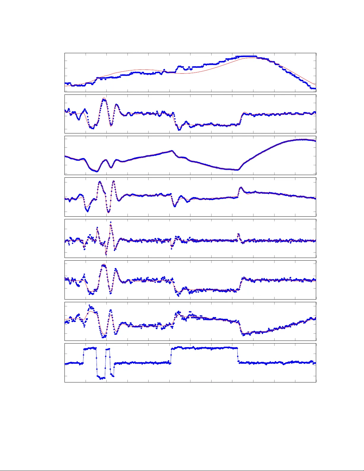
Collocation-Based Output-Error Method for Aircraft System Identification

Collocation-Based Output-Err or Method f or Air craft Sy stem Identification Dimas Abreu Arc hanjo Dutra ∗ U niv ersidade F ederal de Minas Ger ais, Belo Horizonte, Minas Gerais, Br azil, 31.270-901 The output-error me thod is a mainsta y of air craft sy stem identification from flight-test data. It is the me thod of c hoice f or a wide range of applications, from the estimation of stability and control deriv atives f or aerodynamic database generation to sensor bias estimation in flight-path reconstruction. Ho w ev er , notable limitations of the output-error method are that it r equir es ad hoc modifications for applications to unst able systems and it is an iterativ e method which is particularl y sensitiv e to the initial guess. In this paper , w e sho w how to r ef ormulate the estimation as a collocation pr oblem, an approac h common in other disciplines but seldomly used in flight v ehicle system identification. Both formulations are equiv alent in terms of ha ving the same solution, but the collocation-based can be applied without modifications or loss of efficiency to unstable systems. Examples with simulated and real-w orld flight-test data also sho w that conv ergence to the optimum is obt ained ev en with poor initial guesses. Nomenclatur e Mathematical symbols R the set of real numbers t time A − 1 matrix inv erse of A A T matrix (or vector) transpose of A Û x time derivativ e of x , i.e., d x / d t C D , C C , C L wind-axis f orce coefficients C ` , C m , C n body-axis moment coefficients n x , n y number of sys tem states and outputs n u , n θ number of sys tem inputs and unkno wn parameters N number of measurement instants in the experiment : = equal by definition, i.e., defined as ln natural logarithm (base e ) det matrix deter minant A cron yms CEA Centro de Estudos Aeronáuticos CEA CoEst CEA Control and Estimation Librar y CPU Central Processing U nit. COIN-OR Computational Infrastructure f or Operations Research. DLR German Aerospace Center . F AA Federal A viation Adminis tration. GPU Graphics Processing U nit. HAR V High Angle of Attac k Researc h V echicle. HA TP High Angle of Attac k T echnology Program. i.i.d. Independent and Identically Distributed. ∗ Adjunct Professor , Departamento de Engenharia Mecânica, A v . Pres. Antônio Carlos, 6627, Member AIAA. 1 IPOPT Interior Point OPTimizer . IVP Initial- V alue Problem. ML Maximum Likelihood. ODE Ordinary Differential Equation. OEM Output-Error Method. SIMD Single Instruction, Multiple Data. I. Introduction A s the need f or building mathematical models of dynamical sys tems from data, kno wn as syst em identification , arises in sev eral application areas, sev eral scientific communities are activ e in the dev elopment of its theory and algorithms, as noted by Ljung [ 1 , Sec. 3] in a recent surve y . The different uses of the identified models and the context of the systems and tests shapes the identification methods. In the sys tems and automatic control community , for e xample, a major need f or system identification was the obtention of models for control [ 1 , Sec. 3.9]. As in their main application onl y the input–output relationship matters, a f ocus can be seen on black -bo x, discrete-time, transfer function models and methods [ 1 – 4 ]. For aircraft system identification, how ev er , a major driver were research aircraft with no v el configurations or operating at previousl y unexplored flight regimes. Notable e xamples of no v el configurations are the lifting-body M2 prototypes and HL -10, tilt-wing X C-142A, thr ust-v ectored X -31, human-po w ered Gossamer Albatross, and the activ e aeroelastic wing prog ram. Among previousl y unexplored flight regimes we hav e hypersonic speeds as in the X -15 and the space shuttle; and high angles of attack w hich w ere studied in the High Angle of Attac k T echnology Program (HA TP), the F-18 High Angle of Attac k Researc h V echicle (HAR V), and in the X -29. F or more details on these aircraft and the role of sys tem identification in their programs, consult the revie ws and retrospectives of the area in Ref s. 5 – 9 and the ample references therein. The inv estigativ e nature of these programs fa v ored parameter estimation techniques that allo w ed for a deeper understanding of the underl ying aerodynamic phenomena, their relationship to the aircraft stability and control, and the validity of the theoretical and wind-tunnel results. System identification w as also a suppor ting technique in the saf e expasion of the operational flight env elope. T o some e xtent, these needs are also present in the flight-testing of production aircraft prototypes, for which sys tem identification is also routinely used [ 10 , 11 ]. For these, the estimated stability and control der iv ativ es are also used to build high-fidelity aerodynamic databases f or training, engineer ing and in-flight simulators meeting the F AA requirements. Finally , the identified models are also used for control law synthesis and controller tuning. Consequentl y , f or flight v ehicle system identification the focus has been on white-box or light-g ra y -bo x phenomenological models, whose parameters ha v e phy sical meaning and can be related across different reference flight conditions. Most models are multiple-input multiple-output and are represented in the state-space f orm. With respect to the estimation algorithms, for aircraft the maximum likelihood (ML) estimators ha v e dominated. Of these, the output-error method (OEM), which amounts to a nonlinear w eighted least-squares problem when the noise co v ariance matr ix is assumed known is the most widel y used [ 9 , p. 681], ev en for applications such as flight-path reconstruction [ 12 ] and aeroelastic modeling [ 13 , 14 ]. Notable limitations of the classical OEM, ho w e v er , are its inapplicability to unstable sys tems [ 15 ; 11 , Chap. 9] and its conv ergence to local minima when poor initial estimates are used. A field with similar requirements f or system identification as f or flight vehicles is chemical engineer ing, in which the output er ror method w as also dev eloped independently ∗ [ 16 – 20 ]. Their applications also required estimation of parameters of white-bo x continuous-time models in state-space, usually reaction rates in chemical equations. The application of the maximum likelihood pr inciple to this class of problems leads, naturally , to the output-error method. Differences in their application conte xt, how ev er , resulted in alter nativ e implementations routes. Some estimation problems in chemical engineering inv olv e ill-conditioned differential equations which may not hav e a valid solution f or some parameter values. Additionall y , not much a-pr iori information is av ailable on the parameters for the initial guess of iterative methods. This should be contrasted with aircraft parameter estimation, for which reasonably good guesses f or the stability and control der ivativ es can be obtained from theoretical analy ses, wind-tunnel e xperiments and computational-fluid-dynamics calculations. As a result, the chemical reaction system identification community dev eloped implementations of the OEM capable of coping with these issues: multiple shooting and collocation [ 17 , 18 ]. In these approaches to implement the output-er ror ∗ The author’ s search did not yield any references to the aircraft literature when the OEM w as dev eloped in the chemical engineer ing literature. 2 method, the decision variables of the optimization problem are augmented with the states at sev eral mesh points across the e xperiment time inter val. Equality constraints are then added to encode the sys tem dynamics and enf orce continuity of the solution. These methods are also v ery common in optimal control [ 21 ], as there is a cer tain duality between estimation and control, and w ere dev eloped by researchers active in both fields like H. G. Bock [ 22 ]. The author has also used collocation methods in state and parameter estimation problems [ 23 , 24 ]. T raditionally , in the aeronautical literature, the output-error method is implemented using the single shooting or initial-value problem (IVP) approach, in which only the unkno wn parameters and initial v alues of the states are used as decision variables of the nonlinear optimization problem. Good e xplanations of the problems that arise with this f ormulation were given by Bock [ 17 , Sec. 8.2; 18 , p. 97]: neglecting the inf ormation of the states by rewriting the problem only in ter ms of the parameters results in a “reinv ersion of the inv erse problem” which spoils “the very nature of the inv erse problem”, leading to a “deterioration of efficiency” and a “substantial loss of stability”. A defining property of the sys tem identification problems is that there is plentiful inf ormation on the states but comparativel y little on the parameters. This information is efficiently exploited by estimation methods implemented with the collocation and multiple-shooting approaches. A notable improv ement allow ed by collocation and multiple shooting to aircraft system identification with the output-er ror method is applicability to unstable systems without ad hoc modifications. The multiple shooting f ormulation has already been applied to unstable flight v ehicles f or that end [ 15 ; 11 , Sec. 9.12], but is generall y shunned in fa v or of the stabilized OEM due to programming comple xity and reuse of exis ting code [ 11 , Sec. 9.15]. Another disadvantag e of the single shooting problem f ormulation with respect to the state-augmented ones is diver g ence of the optimization and con v er g ence to suboptimal local minima. While these issues may not be a problem f or estimation of the r igid-body dynamics, they are an issue for aeroelastic or aeroser v oelastic sys tem identification which f eature larg er and more comple x models with parameters that are more difficult to predict accurately [ 25 , Sec. I]. In this paper , we present the collocation f or mulation of the output-er ror method, which is seldomly used f or sy stem identification of aircraft from flight-test data—one of the fe w ex amples av ailable was presented b y Betts [ 21 , Sec. 7.4 ] . The method is applied to e xperimental and simulated flight data bundled with the supplemental mater ial of Jategaonkar [ 11 ] and ground vibration test data from the experiment descr ibed by Gupta et al. [ 26 ] . The conv er g ence basin of the collocation implementation is e xplored to inv estigate its robustness agains t poor star ting v alues f or the parameters. This paper is organized as follo ws. In Sec. II , the output-er ror method is presented, together with the three main approaches to implement it: single shooting, multiple shooting and collocation. In Sec. III the proper ties of the collocation implementation are illustrated with three e xamples. Finally , in Sec. IV the conclusions are drawn out and directions f or future work are outlined. II. The output-error method In this section w e f ormulate the output-error method f or parameter estimation and descr ibe the three main implementations used to write it as a nonlinear optimization problem in a form suitable f or computational solution. A. Problem formulation 1. Gener al case The g eneral problem consists of estimating the vector of unkno wn parameters θ ∈ R n θ of a system descr ibed by ordinary differential equations (ODEs) of the f orm Û x ( t ) = f  x ( t ) , u ( t ) , θ  , x ( 0 ) = x 0 ( θ ) , (1) where t ∈ R is the time, x : R → R n x is the state-path of the system, u : R → R n u are the e xternal inputs, f : R n x × R n u × R n θ → R n x is a possibly nonlinear function encoding the sys tem dynamics, and x 0 : R n θ → R n x is the initial state of the e xperiment which is, without loss of generality , assumed to start at t = 0 . The parameter vector θ holds all unkno wn system parameters, which may include aerodynamic stability and control der ivativ es, initial states, sensor bias, and ev en parameters of the stochas tic noise model such as variance. The sys tem outputs y : R → R n y are described by a static function g : R n x × R n u × R n θ → R n y which can also depend on the unknown parameters, y ( t ) = g  x ( t ) , u ( t ) , θ  . (2) 3 While the outputs y represent the ideal measurables, we onl y hav e access to the measurements z k , sampled at a finite number N of time instants ˜ t k . Under the statistical framew ork of maximum likelihood estimation, the z k are inter preted as noise-corr upted measurements of the outputs, z k = y ( ˜ t k ) + e k , where the measurement noise e k is descr ibed b y some suitable probability distribution. The maximum likelihood estimate ˆ θ ML is then the value which maximizes the likelihood function: the joint conditional probability density p z 1 : N of all measurements, giv en the parameters ˆ θ ML : = arg max θ p z 1 : N  z 1 , . . . , z N   θ  . (3) U nder the assumption that the noise is idenpendent and identicall y distr ibuted (i.i.d.) across measurement instants, Eq. ( 3 ) can be simplified b y noting that p z 1 : N  z 1 , . . . , z N   θ  = N Ö k = 1 p e  z k − ˆ y ( ˜ t k , θ )   θ  , where p e (· | θ ) is the conditional probability density of the noise vectors e k and ˆ y ( t , θ ) is the predicted sys tem output f or a giv en value of θ , i.e., the solution of Eqs. ( 1 ) and ( 2 ), Û ˆ x ( t , θ ) = f  ˆ x ( t , θ ) , u ( t ) , θ  , ˆ x ( 0 , θ ) = x 0 ( θ ) , ˆ y ( t , θ ) : = g  ˆ x ( t , θ ) , u ( t ) , θ  . As the logarithm is a monotonic function which does not change the location of maxima, the logarithm of the likelihood function, known as the log-likelihood, is usually maximized in ( 3 ) as it leads to better-conditioned problems: ` ( θ ) : = ln p z 1 : N ( z 1 , . . . , z N | θ ) = N Õ k = 1 ln p e  z k − ˆ y ( ˜ t k , θ )   θ  = N Õ k = 1 ` e ( z k − ˆ y ( ˜ t k , θ ) , θ ) , ` e (  , θ ) : = ln p e (  | θ ) . The most general form of the output-er ror method estimation problem is then maximize θ ∈ R n θ N Õ k = 1 ` e ( z k − ˆ y ( ˜ t k , θ ) , θ ) (6a) subject to ˆ x ( 0 , θ ) = x 0 ( θ ) (6b) Û ˆ x ( t , θ ) = f  ˆ x ( t , θ ) , u ( t ) , θ  (6c) ˆ y ( t , θ ) = g  ˆ x ( t , θ ) , u ( t ) , θ  . (6d) 2. Special case: Gaussian measurement noise Due to the tractability of the maximization problems it produces and its ubiquity in statis tical models, the noise is often assumed to be zero-mean and normally distributed. In that case, denoting by R : R n θ → R n y × n y its cov ariance matrix, e k ∼ N  0 , R ( θ )  k = 1 , . . . , N , the noise log-density is ` e (  , θ ) = − 1 2  T R ( θ ) − 1  − 1 2 ln det  R ( θ )  − n y 2 ln ( 2 π ) . (7) 4 When the noise co v ariance is kno wn or fix ed ( R does not depend on θ ), the last tw o ter ms in the right-hand side of ( 7 ) can be dropped as they are constants which do not influence the location of maxima. The maximum likelihood estimator reduces to a nonlinear w eighted least-squares problem with R − 1 as the w eighting matr ix, minimize θ ∈ R n θ N Õ k = 1  z k − ˆ y ( ˜ t k , θ )  T R − 1  z k − ˆ y ( ˜ t k , θ )  (8a) subject to ˆ x ( 0 , θ ) = x 0 ( θ ) (8b) Û ˆ x ( t , θ ) = f  ˆ x ( t , θ ) , u ( t ) , θ  (8c) ˆ y ( t , θ ) = g  ˆ x ( t , θ ) , u ( t ) , θ  , (8d) in which the sign of ` was inv er ted and the maximization conv erted to a minimization. If, fur thermore, the elements of the noise v ector e k are assumed to be independent of each other , then R is diagonal, R =           r 1 0 · · · 0 0 r 2 · · · 0 . . . . . . . . . . . . 0 0 · · · r n y           and the maximum likelihood estimation problem is minimize θ ∈ R n θ N Õ k = 1 n y Õ i = 1  z k − ˆ y ( ˜ t k , θ )  2 i r i (9a) subject to ˆ x ( 0 , θ ) = x 0 ( θ ) (9b) Û ˆ x ( t , θ ) = f  ˆ x ( t , θ ) , u ( t ) , θ  (9c) ˆ y ( t , θ ) = g  ˆ x ( t , θ ) , u ( t ) , θ  , (9d) in which [  ] i denotes the i -th element of the  vector . 3. A pr agmatic view on the statistical model W e note that although the maximum likelihood estimator is der ived from a statiscal framew ork f or which it is an optimal solution, it makes sense regardless of the probabilistic iterpretation [see 4 , pp. 16, 222]. From a pragmatic vie wpoint, we could regard the noise log-density ` e in ( 6a ) as a metr ic or norm on the er ror size. In ( 8a ) and ( 9a ) , for e xample, the estimate minimizes the mean squared Mahalanobis distance between the measurements and the model outputs. When the log-density ` e depends on the parameter θ as in ( 7 ) , the “best” metric is not known bef orehand [ 4 , p. 200] so it is chosen by the help of a cr iterion which penalizes “small” metrics, e.g., the ln det  R ( θ )  term of ( 7 ). The choice of the output noise distribution p e can then be transformed to the choice of a metr ic L : R n y × R n θ → R f or the er ror size in the optimization problem minimize θ ∈ R n θ N Õ k = 1 L ( z k − ˆ y ( ˜ t k , θ ) , θ ) (10a) subject to ˆ x ( 0 , θ ) = x 0 ( θ ) (10b) Û ˆ x ( t , θ ) = f  ˆ x ( t , θ ) , u ( t ) , θ  (10c) ˆ y ( t , θ ) = g  ˆ x ( t , θ ) , u ( t ) , θ  . (10d) The estimation yields the “smallest” mean er ror , acording to L . Sev eral metr ics ha v e emerged as robust alternatives to the quadratic form associated with the normal distribution [ 27 – 31 ]. B. Single shooting implementation The optimization problems in the preceding section, represented in ( 6 ) , ( 8 ) , ( 9 ) and ( 10 ) , are still in an abstract f orm, as the tr ue solution of the ODE ( 1 ) is ref erenced. Ex cept for the case of linear or affine sys tems, the predicted 5 state-path does not admit closed-form solutions. Hence, the most ob vious wa y to implement the output-er ror method is to compute an appro ximate solution of the sys tem state-path by using a numer ical integration scheme like a Rung e–Kutta method. This is known as the single shooting or initial-value problem (IVP) implementation. For a sur v e y of numer ical integration methods as it per tains to aircraft sys tem identification using single shooting, see Jategaonkar [ 11 , Sec. 3.8.1 ] . A single time mesh of m distinct instants τ k of the e xperiment inter val [ 0 , T ] , including the endpoints, is selected to perform the integration: 0 = τ 1 < τ 2 < · · · < τ m = T . W e will assume here that the mesh includes all measurement times ˜ t k , as this simplifies the implementation and notation. Ho w e v er, this is not needed if an associated inter polation scheme (dense output) is used with the integration method [e.g., 32 ]. In an y case, it is impor tant that the mesh be kept fixed dur ing the optimization as its variation f or different θ , which can occur when using variable-step methods, can introduce noise into the objective function and its der ivativ es [ 21 , pp. 44, 110]. Nev er theless, estimates of the integration error are useful to ev aluate the need f or mesh refinement or alternative integration schemes. Let us denote b y I one step of the integration method, ˆ x k + 1 = I ( ˆ x k , τ k , τ k + 1 , u , θ, f ) , (11) i.e., the method applied to the solution of the differential equation defined by f , with the input function u , starting with the v alue ˆ x k at the time τ k and returning the value ˆ x k + 1 corresponding to τ k + 1 . With Euler’ s method, f or example, w e w ould hav e I ( ˆ x k , τ k , τ k + 1 , u , θ, f ) = ˆ x k + ( τ k + 1 − τ k ) f  ˆ x k , u ( τ k ) , θ  . The output-error method is then maximize θ ∈ R n θ N Õ k = 1 τ i = ˜ t k ` e ( z k − ˆ y i , θ ) (12a) subject to ˆ x 1 = x 0 ( θ ) (12b) ˆ x k + 1 = I ( ˆ x k , τ k , τ k + 1 , u , θ, f ) , k = 1 , . . . , m − 1 (12c) ˆ y k = g  ˆ x k , u ( τ k ) , θ  , k = 1 , . . . , m . (12d) Eqs. ( 12b )–( 12d ) are e xplicit and can be calculated one after the other, iterativ el y . When the f , g and ` e functions are continuous and differentiable the problem is amenable to solution with Ne wton ’ s method. The gradients can be obtained by finite differences [ 11 , Sec. 4.8], automatic differentiation or symbolic differentiation of the model functions. The resulting nonlinear programming problem can then be readil y sol v ed with a wide range of av ailable software packag es like the open-source IPOPT from the COIN-OR initiativ e [ 33 ]. If the Gaussian distribution is assumed for the measurement error in the f orm of ( 7 ) , ( 8 ) or ( 9 ) , nonlinear least-squares optimization methods such as the Gauss–Ne wton or Lev enberg–Marquardt algor ithms can be used to obtain the solution [ 11 , Sec. 4.6 and 4.13]. The problem is dense but relativ el y small-sized, usually with up to hundreds of decision variables which are the elements of the unkno wn parameter vector θ . Ho w e v er, it should be noted that the numer ical solution of the differential equation might div erg e or deviate far from the measurements f or parameter values far from the optimum. This can, in tur n, lead to diver g ence of the optimization or con v er g ence to suboptimal local maxima. Further more, in unstable, marginally stable, poorl y damped or sy stems with slo w dynamics the er rors in the integ ration method can accumulate or be amplified by the sys tem dynamics, degrading the estimates. C. Multiple shooting implementation In the multiple shooting implementation [ 17 ; 18 ; 11 , Sec. 9.12] of the output-er ror method, a numer ical integration scheme is used as in the single shooting approach, but divided into multiple segments with independent initial states which are appended to the decision variables of the optimization. Equality constraints are then included to enf orce continuity of the state solution across segments. By the choice of a gr id 0 = t ( 1 ) < t ( 2 ) < · · · < t ( n s + 1 ) = T . (13) 6 the e xperiment inter val is divided into n s segments, each of which is fur ther subdivided b y a finer mesh of m k points f or numerical integ ration, t ( k ) = τ ( k ) 1 < τ ( k ) 2 < · · · < τ ( k ) m k = t ( k + 1 ) , k = 1 , . . . , n s . (14) The v ector ξ of decision variables of the optimization is then augmented with the state at the beginning of each segment after the first, ξ = h θ ˆ x ( 2 ) 1 ˆ x ( 3 ) 1 · · · ˆ x ( n s ) 1 i and the state equations ( 1 ) are integ rated using the chosen numer ical scheme along the mesh of each segment, independently . Using the same notation for the integration scheme as in ( 11 ) , the multiple shooting approach f or the output-er ror method is maximize θ, ˆ x ( 2 ) 0 , . . . , ˆ x ( n s ) 0 N Õ k = 1 τ ( j ) i = ˜ t k ` e  z k − ˆ y ( j ) i , θ  (15a) subject to ˆ x ( 1 ) 1 = x 0 ( θ ) (15b) ˆ x ( i ) k + 1 = I ( ˆ x ( i ) k , τ ( i ) k , τ ( i ) k + 1 , u , θ, f ) , k = 1 , . . . , m i − 1; i = 1 , . . . , n s (15c) ˆ y ( i ) k = g  ˆ x ( i ) k , u ( τ ( i ) k ) , θ  , k = 1 , . . . , m i ; i = 1 , . . . , n s (15d) ˆ x ( i ) m k − ˆ x ( i + 1 ) 1 = 0 i = 1 , . . . , n s − 1 . (15e) Eqs. ( 15b ) – ( 15d ) are explicit and can be calculated one after the other , iterativel y . In addition, the iterations of each segment i are independent, per mitting a considerable speedup when using moder n computer hardw are with parallel capabilities. Finall y , we note that ( 15e ) are the continuity constraints, requir ing that the final point of each segment coincide with the initial point of the next. They are, generall y , nonlinear functions of the decision variables ev en f or linear dynamical sys tems. The optimization problem resulting from ( 15 ) is larg er , due to the inclusion of the additional variables and constraints, but it is sparse. This method is far more robust against diver g ence of the numer ical solution to the differential equation than single shooting. As each segment is kept shor t, e v en when f or inadequate parameter values, the solution does not deviate much from the first point of the segment. Fur thermore, from the very inv erse nature of the in v erse problem, more inf or mation on the states is usually av ailable than on the parameters, allowing f or better star ting v alues f or the optimization. The continuity constraints are enf orced by the optimization solv er with a small tolerance which can offset the integration er rors accumulated on unstable, marginall y stable or poorl y damped systems. This allow s the method to be used without modifications on this impor tant class of systems, yielding good results. Fur thermore, the e xpansion of the search domain gives more degrees of freedom to the optimization solv er , which can no w explore search directions which violate the continuity constraints. This endow s the method with better numer ical and conv er g ence proper ties, allo wing it to ov ercome local minima which w ould other wise capture the single shooting implementation. D. Collocation implementation The collocation approach f or f ormulating the output-er ror method consists of adding all (or most) state points used b y the integ ration scheme as decision v ariables of the optimization and encoding the integration method as equality constraints. Instead of iterating the integration scheme, the integration error of the candidate solution is ev aluated and passed on to the optimization routine, which dr iv es it to zero at the same time it w orks to maximize the objective. Because of this, implicit integration schemes are a natural choice f or collocation methods. The method is very general with many variations, so we will e x emplify it here with a famil y of Lobatto methods which includes the trapezoidal method. A v ery thorough ref erence on collocation methods f or parameter estimation, with implementation details and ex amples is Betts [ 21 ] . Additional inf ormation can also be f ound in the works of Betts and Huffman [ 34 ] and Williams and T rivailo [ 35 ]. Like in the multiple shooting, the experiment inter val is divided into a g rid of n s segments ( 13 ) , each of which is fur ther subdivided into a finer mesh ( 14 ) of m k points, including the endpoints. The vector ξ of decision variables of the 7 optimization problem is then augmented with the state at all mesh points, ξ = h θ ˆ x ( 1 ) 1 · · · ˆ x ( 1 ) m 1 ˆ x ( 2 ) 2 · · · ˆ x ( 2 ) m 2 ˆ x ( 3 ) 2 · · · ˆ x ( 3 ) m 3 · · · ˆ x ( n s ) m n s i . Notice that the end of each segment coincides with the star t of the ne xt, but only one decision variable is needed to represent it. T o simplify notation in what f ollo w s, we will use both ˆ x ( i ) m i and ˆ x ( i + 1 ) 1 to ref er to these variables. T o der iv e the method, we first note that both sides of the differential equation ( 1 ) can be integ rated, leading to the integral f orm of the system equations: x ( t b ) − x ( t a ) = ∫ t b t a f  x ( τ ) , u ( τ ) , θ  d τ ∀ t a , t b ∈ [ 0 , T ] . (16) This integ ral relation holds for an y tw o time values in the e xperiment interval. A wa y of appro ximating this relation is to build a polynomial appro ximation ˆ f ( t ) of the function f at the mesh points and enf orce ( 16 ) to hold f or ˆ f and an y pair t a , t b in the mesh. Let λ ( i ) k ( t ) denote the k -th Lag rang e basis polynomial f or the mesh of the i -th segment: λ ( i ) k ( t ) = Ö 1 ≤ j ≤ m i j , k t − τ ( i ) j τ ( i ) k − τ ( i ) j . This basis is defined such that λ ( i ) k ( τ ( i ) k ) = 1 , λ ( i ) k ( τ ( i ) j ) = 0 , ∀ j , k , simplifying the construction of a polynomial inter polant of f at the g rid points: ˆ f ( i ) ( t ) = m i Õ k = 1 λ ( i ) k ( t ) f  ˆ x ( i ) k , u ( τ ( i ) k ) , θ  . If we apply the integ ral form of the system equation ( 16 ) to ˆ f , we obtain the collocation constraints for this famil y of Lobatto methods: ˆ x ( i ) k + 1 − ˆ x ( i ) k = ∫ τ ( i ) k + 1 τ ( i ) k ˆ f ( i ) ( τ ) d τ = m i Õ j = 1 f  ˆ x ( i ) j , u ( τ ( i ) j ) , θ  ∫ τ ( i ) k + 1 τ ( i ) k λ ( i ) j ( τ ) d τ . (17) W e note that the last integ ral on the r ight-hand side of ( 17 ) depends only on the location of the mesh points and can be calculated bef orehand C ( i ) j , k : = ∫ τ ( i ) k + 1 τ ( i ) k λ ( i ) j ( τ ) d τ . Further more, as the integral of a polynomial it has a simple analytic solution. The mesh points must be carefully chosen to av oid Rung e ’ s phenomenon and guarantee a low bound on the solution er ror . A good general choice are the Legendre–Gauss–Lobatto nodes of the segment [ 35 , Sec. 3]. The collocation-based output-error method then amounts to the follo wing optimization problem maximize θ, ˆ x ( 1 ) 1 , . . . , ˆ x ( 1 ) m 1 , ˆ x ( 2 ) 2 , . . . , ˆ x ( n s ) m n s N Õ k = 1 τ ( j ) i = ˜ t k ` e  z k − ˆ y ( j ) i , θ  (18a) subject to 0 = ˆ x ( 1 ) 1 − x 0 ( θ ) (18b) 0 = ˆ x ( i ) k + 1 − ˆ x ( i ) k − m i Õ j = 1 f  ˆ x ( i ) j , u ( τ ( i ) j ) , θ  C ( i ) j , k , k = 1 , . . . , m i − 1; i = 1 , . . . , n s (18c) ˆ y ( i ) k = g  ˆ x ( i ) k , u ( τ ( i ) k ) , θ  , k = 1 , . . . , m i ; i = 1 , . . . , n s . (18d) 8 Of the three approaches presented in this section, collocation leads to the larges t optimization problem, but also the most sparse. Both the objectiv e function and the constraints are very simple and can be parallelly ev aluated. Each segment ’ s mesh and length is usually kept small, such that there is little variation of the state and inputs within it, which makes the linear ization of the constraints b y sequential quadratic prog ramming sol v ers reasonable approximations. When most states are measured, good initial values of the states can be used f or the optimization, improving conv er g ence ev en starting with inadequate parameter values. The same considerations made on the end of Sec. II.C about the multiple shooting approach also apply here, ev en to a higher deg ree. Diver g ence of the numer ical integ ration does not make sense unless the whole v ector of decision variables diver ges. The er ror tolerance on the constraint violation prev ents integration error from accumulating ev en in a single integration step. The segments are ev en smaller and the collocation constraint is closer to a linear function, as the function f is not applied recursiv el y into itself. This makes the problem more amenable to solution with Ne wton’ s method, which emplo y s quadratic approximations f or the objective and linear approximations f or the constraints. III. Examples W e illustrate the collocation-based output-er ror method with three experiments: a linear model parameter estimation of the shor t per iod dynamics from a simulated unstable aircraft; a nonlinear longitudinal model estimation of a HFB-320 Hansa Jet from e xperimental data collected by the DLR; and a high order (24 states) black -bo x linear model estimation from an e xperimental ground vibration test of a unmanned flexible flying wing aircraft. The e xamples were chosen to demonstrate the robustness of the collocation approach to poor start parameters; its applicability , without modifications, to parameter estimation in unstable sys tems; and its use in a challenging larg e-scale problem, with sev eral states and man y samples, typical of fle xible vehicle parameter estimation. The source code of the analy ses per f or med f or this article were released as open-source software † . The estimation routines were implemented in the open-source CEA Control and Estimation Librar y (CEA CoEst) ‡ , under dev elopment by the author . It is wr itten in the Python prog ramming language and uses the open-source large-scale interior point nonlinear optimization solv er IPOPT [ 33 ], part of the COIN-OR initiativ e. The solv er, in tur n, uses the efficient sparse linear sys tem sol v ers of the HSL Mathematical Software Library § to obtain the search direction of Ne wton’ s method. The HSL and OpenBLAS [ 36 ] librar ies in the implementation used were compiled with the OpenMP parallel computing frame w ork [ 37 ] enabled, exploiting the parallelism inherent in the collocation f ormulation. A. HFB-320 Hansa Jet longitudinal motion Experimental data collected from a HFB-320 Hansa Jet aircraft by the DLR are a v ailabe with the supplemental material ¶ of the book b y Jategaonkar [ 11 ]. It consists of an elev ator 3-2-1-1 input f ollo wed by a pulse. A nonlinear model was estimated with 4 states, the airspeed V , angle of attack α , pitch angle ϑ , pitch rate q ; 2 inputs, the elev ator deflection δ e and the thrust f orce T ; and 7 measurements, ˜ V , ˜ α , ˜ ϑ , ˜ q and the pitch acceleration ˜ a q , longitidinal acceleration ˜ a x , and v ertical acceleration ˜ a z . A total of 28 unknown parameters θ w ere estimated: the dimensionless stability and control der ivativ es C D 0 , C D V , C D α , C L 0 , C L V , C L α , C m 0 , C m V , C m α , C m q , and C m δ e ; the measurement biasses b q , b a q , b a x , and b a z ; the measurement noise standard deviations σ V , σ α , σ ϑ , σ q , σ a q , σ a x , and σ a z ; and the initial states V 0 , α 0 , θ 0 , and q 0 . The function f of the dynamics is defined by the follo wing relations: Û V = − ρ S 2 m V 2  C D 0 + C D V ( V V ref − 1 ) + C D α α  + T m cos ( α +  T ) − g 0 sin ( θ − α ) Û α = − ρ S 2 m V  C L 0 + C L V ( V V ref − 1 ) + C L α α  − T mV sin ( α +  T ) + g 0 V cos ( θ − α ) + q Û ϑ = q Û q = ρ S ¯ c 2 I y V 2  C m 0 + C m V ( V V ref − 1 ) + C m α α + C m q ¯ c q 2 V + C m δ e δ e  + ` T I y T . † A vailable for download at https://github.com/dimasad/aviation- 2019- code ‡ A vailable for download at https://github.com/cea- ufmg/ceacoest § HSL. A collection of Fortran codes for large scale scientific computation. http://www.hsl.rl.ac.uk/ ¶ Freely available for download at https://arc.aiaa.org/doi/suppl/10.2514/4.102790 9 parameter low er starting value upper star ting v alue optimal C D 0 0 0 . 5 0 . 0580 C D V − 0 . 5 0 . 5 − 0 . 0316 C D α 0 1 0 . 2453 C L 0 0 2 0 . 1808 C L V − 2 2 0 . 2012 C L α 0 10 3 . 0904 C m 0 0 0 . 5 0 . 1184 C m V 0 0 . 5 0 . 0137 C m α − 5 1 − 0 . 9941 C m q − 50 0 − 28 . 6517 C m δ e − 10 0 − 1 . 4714 T able 1 Limits of the uniform distribution from which the st arting parameters of the HFB-320 exam ple w ere dra wn, together with their optimal values. Similarl y , the function g of the outputs is defined by ˜ V = V ˜ α = α ˜ ϑ = ϑ ˜ q = q + b q ˜ a q = b a q + ρ S ¯ c 2 I y V 2  C m 0 + C m V ( V V ref − 1 ) + C m α α + C m q ¯ c q 2 V + C m δ e δ e  + ` T I y T ˜ a x = b a x + ρ S 2 m V 2 h sin α  C L 0 + C L V ( V V ref − 1 ) + C L α α  − cos α  C D 0 + C D V ( V V ref − 1 ) + C D α α  i + T m cos (  T ) ˜ a z = b a z + ρ S 2 m V 2 h − cos α  C L 0 + C L V ( V V ref − 1 ) + C L α α  − sin α  C D 0 + C D V ( V V ref − 1 ) + C D α α  i − T m sin (  T ) . Finall y , the ` e log-density associated with Gaussian noise ( 7 ) was used, with a diagonal R ( θ ) consisting of the measurement variances σ 2 V to σ 2 a z . The estimation was performed a total of 1000 times with random star ting values f or the stability and control derivativ es, drawn from uniform distributions whose intervals are shown in T ab. 1 . The starting value for the bias parameters were zero and for the noise standard deviations was one. The mesh states were initialized with the measured values. Of all starting points of the optimization, 98 . 6 % con v er g ed to the global optimum whose parameter values are listed in the last column of T ab. 1 and model outputs are shown in Fig. 1 . W e note that the optimization conv erg es e v en for very bad v alues of θ which pose problems for the single shooting implementation. Particularl y , if we set all aerodynamic der ivativ es to zero, there is no lift, drag or aerodynamic pitching moment and the model plummets down, its initial-value problem simulation div er ging. Ho w e v er, the collocation-based estimation manages to reach the optimal solution. B. Simulated unstable aircraft short period T o demonstrate that the collocation-based output-er ror method can be used without modifications to estimate unstable dynamics, we apply it on data from an unstable simulated aircraft. The data was used by Jategaonkar [ 11 , Sec. 9.16.1 ] to compare v arious methods f or unstable aircraft system identification. It should be noted that, f or this sys tem, the initial-value problem approach f or the output-er ror method obtains v ery poor estimates. A linear model of the shor t period dynamics was used with 2 states, the vertical velocity w and pitch rate q ; only 1 input, the elev ator deflection δ e ; and 3 outputs, ˜ w , ˜ q , and the vertical acceleration ˜ a z . A total of 11 parameters were estimated, the dimensional stability and control der ivativ es Z w , Z q , Z δ e , M w , M q , and M δ e ; the measurement noise 10 104 106 108 110 112 V [ m / s ] 5 6 7 α [ ° ] 2 4 6 8 10 θ [ ° ] − 2 0 2 q [ ° / s ] − 5 0 5 a q [ ° / s 2 ] 0 . 8 1 1 . 2 a x [ m / s 2 ] − 11 − 10 − 9 − 8 a z [ m / s 2 ] 0 5 10 15 20 25 30 35 40 45 50 55 60 − 1 − 0 . 5 0 t [ s ] δ e [ ° ] Fig. 1 Estimation results for the HFB320 data. The marks are the measured values and the solid lines are the estimated model output. The ele v ator input for the manuev er is the bottommost plot. 11 − 2 0 2 w [ m / s ] − 10 0 10 q [ ° / s ] − 5 0 5 a z [ m / s 2 ] 0 1 2 3 4 5 6 7 8 9 10 11 12 − 5 0 5 t [ s ] δ e [ ° ] Fig. 2 Estimation results for the simulted unstable aircraft data. The marks are the measured values and the solid lines are the estimated model output. The elev ator input f or the manuev er is the bottommost plot. standard deviations σ w , σ q , and σ a z ; and the initial states w 0 and q 0 . The sys tem dynamics is defined by Û w = Z w w + ( U 0 + Z q ) q + Z δ e δ e , Û q = M w w + M q q + M δ e δ e , and its outputs b y ˜ w = w , ˜ q = q , ˜ a z = Z w w + Z q q + Z δ e δ e . The ` e log-density associated with Gaussian noise ( 7 ) was used, with a diagonal R ( θ ) consisting of the measurement variances σ 2 w to σ 2 a z . The star ting mesh states were the measured values, the stability and control der ivativ es were zero, and the measurement noise standard de viations w ere one. The estimation model outputs for the collocation-based output-error method are shown in Fig. 2 . C. Black -bo x high-order ground vibration test For the estimation of models of the r igid-body flight dynamics of aircraft, most states are measured directl y and the model structure is w ell-kno wn. The estimation of flexible aircraft dynamics poses additional challeng es as the structural states are not usually measured and the model order is much larger . Many of these issues also ar ise in the system identification of str uctural models from g round vibration tests. T o illustrate the application of the collocation-based output-er ror method to this class of problems, it w as applied to accelerometer data from a ground vibration test repor ted b y Gupta et al. [ 26 ], par t of the Perf ormance Adaptiv e Aeroelastic Wing prog ram ‖ . A single-input single-output model with 24 states was estimated f or the force input u and acceleration output y . The ‖ http://www.paaw.net/ 12 ω 1 ω 2 ω 3 ω 4 ω 5 ω 6 199 . 06 186 . 17 178 . 44 172 . 64 144 . 37 121 . 47 ω 7 ω 8 ω 9 ω 10 ω 11 ω 12 96 . 52 59 . 57 58 . 57 59 . 03 48 . 99 48 . 90 T able 2 Starting values for the pole frequencies in the ground vibration test exam ple. 10 15 20 25 30 35 − 60 − 40 − 20 0 20 f [Hz] Gain [dB] Frequency response Empirical estimate OEM estimated model Fig. 3 Frequency response magnitude of the empirical transf er function estimate and of the OEM-estimated model f or the ground vibration test. dynamics w ere represented in the state-space modal f orm: Û x 1 a = σ 1 x 1 a + ω 1 x 1 b + b 1 u Û x 1 b = − ω 1 x 1 a + σ 1 x 1 b . . . Û x 12 a = σ 12 x 12 a + ω 12 x 12 b + b 12 u Û x 12 b = − ω 12 x 12 a + σ 12 x 12 b , such that the sys tem poles are located at σ i ± j ω i . The sy stem output equation is y = c 1 a x 1 a + c 1 b x 1 b + · · · + c 12 a x 12 a + c 12 b x 12 b . The ` e log-density associated with Gaussian noise ( 7 ) was used, with R ( θ ) = σ 2 y . The unknown parameter v ector consists of the pole locations σ i and ω i , the measurement standard deviation σ y , and the coefficients b i , c i a , and c i b . The data collected contains high-frequency components which w e do not wish to consider , so both the input and output were filtered with band-pass filters with a passband of 6 Hz to 32 Hz , composed of cascaded 5th-order Butterworth filters. The data was then decimated by 20 f or the estimation, dropping the sampling rate from 2 kHz to 100 Hz . The starting value for the parameters was zero for the σ i and mesh states, one for the c i a , c i b and b i . The starting values of the ω i w ere obtained from the poles of a model identified with the N4SID algor ithm which are shown in T ab. 2 . The frequency response of the identified model is sho wn in Fig. 3 , together with that of the empir ical transfer function estimate from the test data. A portion of the estimated model outputs sho wn agains t the data can also be seen in Fig. 4 . 13 69 69 . 2 69 . 4 69 . 6 69 . 8 70 70 . 2 70 . 4 70 . 6 70 . 8 71 − 0 . 5 0 0 . 5 t [s] Measurement Estimated model output Fig. 4 P ortion of the time-response of the identified model in the ground vibration test example. IV . Conclusions and future wor k The collocation-based output-er ror method f or parameter estimation, although seldomly used in aircraft system identification, better e xploits the nature of the inv erse problem and has advantag es ov er the ubiquitous single shooting implementations: applicability to a wider class of sys tems, such as unstable, marginall y stable or poorl y damped sys tems; better numer ical and conv erg ence properties such as robustness against poor parameter values; parallelizable f ormulation of the objective function and constraints which can benefit from moder n computer hardware and capabilities such as single instruction, multiple data (SIMD), multicore central processing units (CPUs), graphics processing units (GPUs) and computer clusters. These proper ties can help ov ercome the challenges in demanding applications like the identification of fle xible aircraft dynamics which pose difficulties to the single shooting method. W e note, how e v er, that the main principle behind the collocation method is fair l y general: augmenting the optimization decision variables with the states and encoding their dynamics as equality constraints. This ov erall technique can also be applied to other more general parameter estimation methods as well, notably the filter-error method, lending it similar impro v ements as for the output-er ror method. Ref erences [1] Ljung, L., “Perspectiv es on system identification, ” Annual Review s in Control , V ol. 34, No. 1, 2010, pp. 1–12. doi: 10.1016/j.arcontrol.2009.12.001. [2] Åström, K. J., and T orsten, B., “Numerical Identification of Linear Dynamic Systems from Normal Operating Records, ” IF A C Proceedings V olumes , V ol. 2, No. 2, 1965, pp. 96–111. doi:10.1016/S1474- 6670(17)69024- 4. [3] Åström, K. J., and Eykhoff, P ., “System identification—A sur v e y , ” Automatica , V ol. 7, No. 2, 1971, pp. 123–162. doi: 10.1016/0005- 1098(71)90059- 8. [4] Ljung, L., Syst em Identification: Theor y for the User , 2 nd ed., Prentice Hall, Englew ood Cliffs, Ne w Jersey , 07632, 1999. [5] Klein, V ., “Estimation of aircraft aerodynamic parameters from flight data, ” Prog r ess in Aerospace Sciences , V ol. 26, No. 1, 1989, pp. 1–77. doi:10.1016/ 0376- 0421(89)90002- X. [6] Hamel, P . G., and Jategaonkar , R. V ., “Ev olution of Flight V ehicle Sys tem Identification, ” Jour nal of Aircr aft , V ol. 33, No. 1, 1996, pp. 9–28. doi:10.2514/ 3.46898. [7] W ang, K. C., and Iliff, K. W ., “Retrospectiv e and Recent Examples of Aircraft Parameter Identification at NAS A Dr yden Flight Researc h Center , ” Journal of Air craft , V ol. 41, No. 4, 2004, pp. 752–764. doi:10.2514/ 1.332. [8] Morelli, E. A., and Klein, V ., “ Application of System Identification to Aircraft at NAS A Langle y Researc h Center , ” Jour nal of Aircr af t , V ol. 42, No. 1, 2005, pp. 12–25. doi:10.2514/ 1.3648. 14 [9] Jategaonkar , R., Fischenberg, D., and von Gr uenhagen, W ., “ Aerodynamic Modeling and System Identification from Flight Data—Recent Applications at DLR, ” Journal of Aircraft , V ol. 41, No. 4, 2004, pp. 681–691. doi:10.2514/1.3165. [10] Klein, V ., and Morelli, E., Aircraft Syst em Identification: Theor y and Practice , No. 213 in AIAA Education Ser ies, AIAA, 1801 Ale xander Bell Drive, Reston, V A 20191, 2006. [11] Jategaonkar , R. V ., Flight V ehicle System Identification: A Time-Domain Methodology , 2 nd ed., No. 216 in Progress in Astronautics and A eronautics, AIAA, 1801 Ale xander Bell Drive, Reston, V A 20191, 2015. doi:10.2514/4.102790. [12] Mulder , J. A., Chu, Q. P ., Sr idhar , J. K., Breeman, J. H., and Laban, M., “Non-linear aircraft flight path reconstruction revie w and new advances, ” Progr ess in aerospace sciences , V ol. 35, No. 7, 1999, pp. 673–726. doi:10.1016/S0376- 0421(99)00005- 6. [13] Sil va, B. G. O., and Mönnich, W ., “Data Gathering and Preliminary Results of the System Identification of a Fle xible Aircraft Model, ” AIAA Atmospheric Flight Mechanics Confer ence , 2011. doi:10.2514/6.2011- 6355. [14] Sil va, B. G. O., and Mönnich, W ., “System Identification of Fle xible Aircraft in Time Domain, ” AIAA Atmospheric Flight Mec hanics Confer ence , 2012. doi:10.2514/6.2012- 4412. [15] Jategaonkar , R. V ., and Thielecke, F ., “Evaluation of Parameter Estimation Methods for Unstable Aircraft, ” Journal of Aircr af t , V ol. 31, No. 3, 1994, pp. 510–519. doi:10.2514/ 3.46523. [16] Swartz, J., and Bremer mann, H., “Discussion of parameter estimation in biological modelling: Algorithms f or estimation and ev aluation of the estimates, ” Jour nal of Mathematical Biology , V ol. 1, No. 3, 1975, pp. 241–257. doi:10.1007/BF01273746. [17] Bock, H. G., “Numerical Treatment of Inv erse Problems in Chemical Reaction Kinetics,” Modelling of Chemical Reaction Sys tems , Spr ing er Ser ies in Chemical Physics, V ol. 18, edited by K. H. Eber t, P . Deuflhard, and W . Jäger , Spr inger , Berlin, Heidelberg, 1981, pp. 102–125. doi:10.1007/978- 3- 642- 68220- 9_8. [18] Bock, H. G., “Recent A dv ances in Parameteridentification T echniques f or O.D.E. ” Numerical T r eatment of Inver se Problems in Differ ential and Integr al Equations , Progress in Scientific Computing, V ol. 2, edited by P . Deuflhard and E. Hairer , Birkhäuser Boston, 1983, pp. 95–121. doi:10.1007/978- 1- 4684- 7324- 7_7. [19] Schlöder , J., and Bock, H. G., “Identification of Rate Constants in Bistable Chemical Reactions, ” Numerical T reatment of Inv erse Problems in Differential and Integr al Equations , Prog ress in Scientific Computing, V ol. 2, edited by P . Deuflhard and E. Hairer , Birkhäuser Boston, 1982, pp. 27–47. doi:10.1007/ 978- 1- 4684- 7324- 7_3. [20] Lohmann, T ., Bock, H. G., and Schloeder , J. P ., “Numerical Methods f or Parameter Estimation and Optimal Exper iment Design in Chemical Reaction Sy stems, ” Industrial & Engineering Chemistry Researc h , V ol. 31, 1992, pp. 54–57. doi:10.1021/ ie00001a008. [21] Betts, J. T ., Practical methods for optimal control and estimation using nonlinear progr amming , 2 nd ed., Adv ances in Design and Control, SIAM, 2010. doi:10.1137/ 1.9780898718577. [22] Bock, H. G., and Plitt, K. J., “ A Multiple Shooting Algor ithm f or Direct Solution of Optimal Control Problems, ” IF AC Proceedings V olumes , V ol. 17, No. 2, 1984, pp. 1603–1608. doi:10.1016/S1474- 6670(17)61205- 9. [23] Dutra, D. A., T eixeira, B. O. S., and Aguirre, L. A., “Maximum a post eriori state path estimation: Discretization limits and their inter pretation, ” Automatica , V ol. 50, No. 5, 2014, pp. 1360–1368. doi:10.1016/j.automatica.2014.03.003. [24] Dutra, D. A. A., T eix eira, B. O. S., and Aguirre, L. A., “Joint maximum a posterior i state path and parameter estimation in stoc hastic differential equations, ” Automatica , 2017, pp. 403–408. doi:10.1016/j.automatica.2017.03.035. [25] Grauer , J. A., and Boucher , M. J., “Real- Time Parameter Estimation f or Fle xible Aircraft, ” AIAA Atmospheric Flight Mechanics Conf er ence , 2018. doi:10.2514/6.2018- 3155. [26] Gupta, A., Seiler, P . J., and Danow sky , B. P ., “Ground Vibration T ests on a Fle xible Flying Wing Aircraft, ” AIAA Atmospheric Flight Mechanics Confer ence , American Institute of Aeronautics and Astronautics, 2016. doi:10.2514/6.2016- 1753. [27] Ara vkin, A., Burke, J., and Pillonetto, G., “Nonsmooth reg ression and state estimation using piecewise quadratic log-conca v e densities, ” IEEE CDC , 2012, pp. 4101–4106. doi:10.1109/ CDC.2012.6426893. [28] Ara vkin, A., Burke, J., and Pillonetto, G., “Robus t and T rend-Follo wing Kalman Smoothers Using Student’ s t, ” SYSID , 2012, pp. 1215–1220. doi:10.3182/ 20120711- 3- BE- 2027.00283. [29] Ara vkin, A., Burke, J., and Pillonetto, G., “ A Statis tical and Computational Theor y for Robust and Sparse Kalman Smoothing, ” SYSID , 2012, pp. 894–899. doi:10.3182/20120711- 3- BE- 2027.00282. 15 [30] Ara vkin, A., Burke, J., and Pillonetto, G., “Sparse/Robus t Estimation and Kalman Smoothing with Nonsmooth Log-Concav e Densities, ” J. Mac h. Learn. Res. , V ol. 14, No. 9, 2013, pp. 2689–2728. [31] Ara vkin, A., Burke, J. V ., Ljung, L., Lozano, A., and Pillonetto, G., “Generalized Kalman smoothing: Modeling and algor ithms, ” Automatica , V ol. 86, 2017, pp. 63–86. doi:10.1016/j.automatica.2017.08.011. [32] Shampine, L. F ., “Inter polation for Rung e-Kutta Methods, ” SIAM Journal on Numerical Analy sis , V ol. 22, No. 5, 1985, pp. 1014–1027. doi:10.1137/0722060. [33] W ächter , A., and Biegler , L. T ., “On the implementation of an interior-point filter line-search algorithm f or larg e-scale nonlinear programming, ” Mathematical Progr amming , V ol. 106, No. 1, 2006, pp. 25–57. doi:10.1007/ s10107- 004- 0559- y. [34] Betts, J., and Huffman, W ., “Larg e Scale Parameter Estimation Using Sparse Nonlinear Programming Methods, ” SIAM Journal on Optimization , V ol. 14, No. 1, 2003, pp. 223–244. doi:10.1137/S1052623401399216. [35] Williams, P ., and T rivailo, P ., “Optimal parameter estimation of dynamical sy stems using direct transcr iption methods, ” Inv erse Problems in Science and Engineering , V ol. 13, No. 4, 2005, pp. 377–409. doi:10.1080/ 17415970500104499. [36] W ang, Q., Zhang, X., Zhang, Y ., and Yi, Q., “A UGEM: Automaticall y Generate High Perf ormance Dense Linear Algebra Kernels on x86 CPUs, ” Proceedings of the International Conf er ence on High P er formance Computing, Ne tw or king, Stor age and Analysis , A CM, Ne w Y ork, NY , USA, 2013, pp. 25:1–25:12. doi:10.1145/ 2503210.2503219. [37] OpenMP Architecture R e vie w Board, “OpenMP Application Program Inter face V ersion 4.0, ” , July 2013. 16