Evaluating Conformance Measures in Process Mining using Conformance Propositions (Extended version)

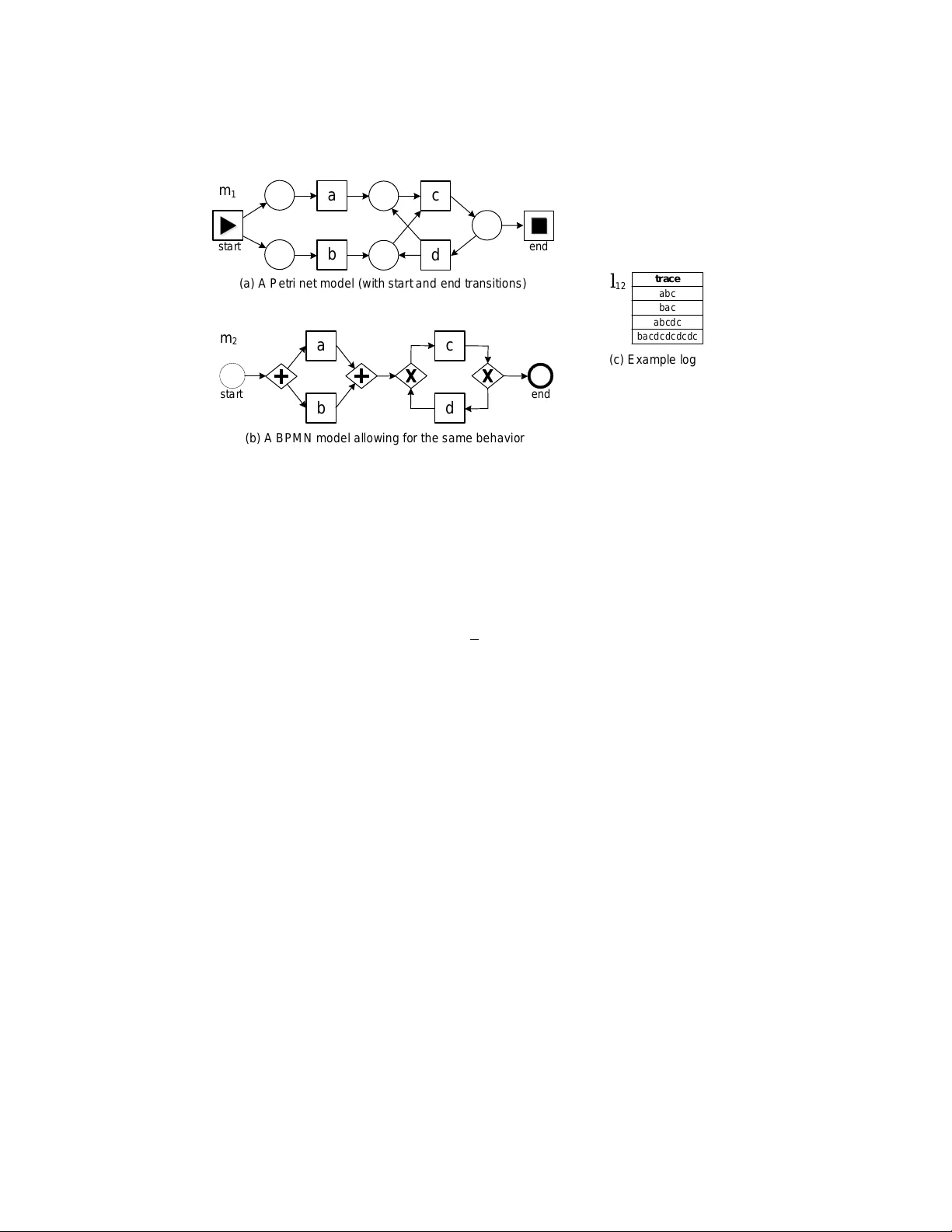
Evaluating Conf ormance Measur es in Process Mining using Conf ormance Propositions (Extended V ersion) Anja F . Syring 1 , Niek T ax 2 , and W il M.P . van der Aalst 1 , 2 , 3 1 Process and Data Science (Informatik 9), R WTH Aachen Univ ersity , D-52056 Aachen, Germany 2 Architecture of Information Systems, Eindhov en University of T echnology , Eindhov en, The Netherlands 3 Fraunhofer Institute for Applied Information T echnology FIT , Sankt Augustin, Germany Abstract. Process mining sheds new light on the relationship between process models and real-life processes. Process discovery can be used to learn process models from ev ent logs. Conformance checking is concerned with quantifying the quality of a business process model in relation to ev ent data that was logged during the execution of the business process. There exist different categories of conformance measures. Recall , also called ﬁtness, is concerned with quantify- ing how much of the beha vior that was observed in the e vent log ﬁts the process model. Precision is concerned with quantifying how much behavior a process model allo ws for that w as ne ver observed in the e vent log. Generalization is con- cerned with quantifying ho w well a process model generalizes to beha vior that is possible in the business process but was never observed in the event log. Many recall, precision, and generalization measures hav e been dev eloped throughout the years, but they are often deﬁned in an ad-hoc manner without formally deﬁn- ing the desired properties up front. T o address these problems, we formulate 21 conformance pr opositions and we use these propositions to ev aluate current and existing conformance measures. The goal is to trigger a discussion by clearly for - mulating the challenges and requirements (rather than proposing new measures). Additionally , this paper serves as an ov erview of the conformance checking mea- sures that are av ailable in the process mining area. Keyw ords: Process mining · Conformance checking · Evaluation measures 1 Introduction Process mining [1] is a fast gro wing discipline that focuses on the analysis of e vent data that is logged during the execution of a business process. Events in such an ev ent log contain information on what was done, by whom, for whom, where, when, etc. Such ev ent data are often readily available from information systems that support the execu- tion of the business process, such as ERP , CRM, or BPM systems. Pr ocess discovery , the task of automatically generating a process model that accurately describes a b usiness process based on such event data, plays a prominent role in process mining. Throughout the years, many process discovery algorithms have been developed, producing process models in various forms, such as Petri nets, process trees, and BPMN. Event logs are often incomplete, i.e., they only contain a sample of all possible be- havior in the b usiness process. This not only mak es process discov ery challenging; it is also difﬁcult to assess the quality of the process model in relation to the log. Process discov ery algorithms take an event log as input and aim to output a process model that satisﬁes certain properties, which are often referred to as the four quality dimensions [1] of process mining: (1) r ecall : the discovered model should allow for the behavior seen in the ev ent log (av oiding “non-ﬁtting” behavior), (2) pr ecision : the discov ered model should not allow for behavior completely unrelated to what was seen in the event log (av oiding “underﬁtting”), (3) generalization : the discov ered model should generalize the example behavior seen in the ev ent log (avoiding “ov erﬁtting”), and (4) simplicity : the discovered model should not be unnecessarily complex. The simplicity dimension refers to Occam’ s Razor: “one should not increase, be yond what is necessary , the num- ber of entities required to explain anything”. In the context of process mining, this is often operationalized by quantifying the complexity of the model (number of nodes, number of arcs, understandability , etc.). W e do not consider the simplicity dimension in this paper, since we focus on behavior and abstract from the actual model repre- sentation. Recall is often referred to as ﬁtness in process mining literature. Sometimes ﬁtness refers to a combination of the four quality dimensions. T o a void later confusion, we use the term recall which is commonly used in pattern recognition, information re- triev al, and (binary) classiﬁcation. Many conformance measures have been proposed throughout the years, e.g., [1,3,5,12,13,14,15,24,25,27,31,32]. So far it remains an open question whether existing measures for recall, precision, and generalization measure what they are aiming to measure. This motiv ates the need for a formal frame work for conformance measures. Users of existing conformance mea- sures should be aware of seemingly obvious quality issues of existing approaches and researchers and dev elopers that aim to create new measures should be clear on what conformance characteristics they aim to support. T o address this open question, this paper ev aluates state-of-the-art conformance measures based on 21 propositions intro- duced in [2]. The remainder is organized as follows. Section 2 discusses related work. Section 3 introduces basic concepts and notations. The rest of the paper is split into two parts where the ﬁrst one discusses the topics of recall and precision (Section 4) and the sec- ond part is dedicated to generalization (Section 5). In both parts, we introduce the corre- sponding conformance propositions and provide an overvie w of existing conformance measures. Furthermore, we discuss our ﬁndings of validating existing these measures on the propositions. Additionally , Section 4 demonstrates the importance of the propo- sitions on sev eral baseline conformance measures, while Section 5 includes a discussion about the different points of vie w on generalization. Section 6 concludes the paper . 2 Related work In early years, when process mining started to gain in popularity and the community around it grew , many process discovery algorithms were developed. But at that time there was no standard method to ev aluate the results of these algorithms and to compare them to the performance of other algorithms. Based on this, Rozinat et al. [28] called on the process mining community to de velop a standard frame work to e valuate process discov ery algorithms. This led to a variety of ﬁtness/recall, precision, generalization and simplicity notions [1]. These notions can be quantiﬁed in different ways and there are often trade-offs between the different quality dimensions. As shown using generic algorithms assigning weights to the different quality dimensions [10], one quickly gets degenerate models when leaving out one or two dimensions. For e xample, it is very easy to create a simple model with perfect recall (i.e., all observed behavior ﬁts perfectly) that has poor precision and provides no insights. Throughout the years, se veral conformance measures ha ve been de veloped for each quality dimension. Ho wever , it is unclear whether these measures actually measure what they are supposed to. An initial step to address the need for a framework to ev aluate conformance measures w as made in [29]. Fi ve so-called axioms for precision measures were deﬁned that characterize the desired properties of such measures. Additionally , [29] showed that none of the existing precision measures satisﬁed all of the formu- lated axioms. In comparison to [29] Janssenswillen et al. [19] did not rely on qualitative criteria, but quantitativ ely compared existing recall, precision and generalization mea- sures under the aspect of feasibility , validity and sensitivity . The results showed that all recall and precision measures tend to behav e in a similar way , while generalization measures seemed to differ greatly from each other . In [2] van der Aalst made a follow- up step to [29] by formalizing recall and generalization in addition to precision and by extending the precision requirements, resulting in a list of 21 conformance propo- sitions. Furthermore, [2] showed the importance of probabilistic conformance mea- sures that also tak e into account trace probabilities in process models. Beyond that, [29] and [2] motiv ated the process mining community to develop new precision mea- sures, taking the axioms and propositions as a design criterion, resulting in the measures among others the measures that are proposed in [26] and in [7]. Using the 21 propo- sitions of [2] we ev aluate state-of-the-art recall (e.g. [4,26,3,16,23,27,33]), precision (e.g. [3,16,17,23,13,26,27,30]) and generalization (e.g. [3,13,16]) measures. This paper uses the mainstream vie w that there are at least four quality dimensions: ﬁtness/recall, precision, generalization, and simplicity [1]. W e deliberately do not con- sider simplicity , since we focus on behavior only (i.e., not the model representation). Moreov er, we treat generalization separately . In a controlled experiment one can assume the existence of a so-called “system model”. This model can be simulated to create a synthetic e vent log used for disco very . In this setting, conformance checking can be re- duced to measuring the similarity between the discovered model and the system model [9,20]. In terms of the well-known confusion matrix, one can then reason about true positiv es, f alse positi ves, true neg atives, and f alse ne gatives. Howe ver , without a system model and just an ev ent log, it is not possible to ﬁnd false positiv es (traces possible in the model but not in reality). Hence, precision cannot be determined in the traditional way . Janssenswillen and Depaire [18] conclude in their ev aluation of state-of-the-art conformance measures that none of the e xisting approaches reliably measures this sim- ilarity . Howe ver , in this paper , we follo w the traditional vie w on the quality dimensions and exclude the concept of the system from our work. Whereas there are many ﬁtness/recall and precision measures there are fewer gen- eralization measures. Generalization deals with future cases that were not yet observed. There is no consensus on how to deﬁne generalization and in [19] it was shown that there is no agreement between existing generalization metrics. Therefore, we cover gen- eralization in a separate section (Section 5). Howe ver , as discussed in [1] and demon- strated through experimentation [10], one cannot leave out the generalization dimen- sion. The model that simply enumerates all the traces in the log has perfect ﬁtness/recall and precision. Ho wev er, ev ent logs cannot be assumed to be complete, thus pro ving that a generalization dimension is needed. 3 Preliminaries A multiset o ver a set X is a function B : X → N which we write as [ a w 1 1 , a w 2 2 , . . . , a w n n ] where for all i ∈ [1 , n ] we have a i ∈ X and w i ∈ N ∗ . B ( X ) denotes the set of all multisets over set X . For example, [ a 3 , b, c 2 ] is a multiset over set X = { a, b, c } that contains three a elements, one b element and two c elements. | B | is the num- ber of elements in multiset B and B ( x ) denotes the number of x elements in B . B 1 ] B 2 is the sum of two multisets: ( B 1 ] B 2 )( x ) = B 1 ( x ) + B 2 ( x ) . B 1 \ B 2 is the difference containing all elements from B 1 that do not occur in B 2 . Thus, ( B 1 \ B 2 )( x ) = max { B 1 ( x ) − B 2 ( x ) , 0 } . B 1 ∩ B 2 is the intersection of two multisets. Hence, ( B 1 ∩ B 2 )( x ) = min { B 1 ( x ) , B 2 ( x ) } . [ x ∈ B | b ( x )] is the multiset of all elements in B that satisfy some condition b . B 1 ⊆ B 2 denotes that B 1 is contained in B 2 , e.g., [ a 2 , b ] ⊆ [ a 2 , b 2 , c ] , but [ a 2 , b 3 ] 6⊆ [ a 2 , b 2 , c 2 ] and [ a 2 , b 2 , c ] 6⊆ [ a 3 , b 3 ] . Process mining techniques focus on the relationship between observed behavior and modeled beha vior . Therefore, we ﬁrst formalize e vent logs (i.e., observed behavior) and process models (i.e., modeled behavior). T o do this, we consider a very simple setting where we only focus on the control-ﬂow , i.e., sequences of acti vities. 3.1 Event Logs The starting point for process mining is an event log. Each event in such a log refers to an activity possibly ex ecuted by a resour ce at a particular time and for a particular case . An ev ent may have many more attributes, e.g., transactional information, costs, cus- tomer , location, and unit. Here, we focus on control-ﬂow . Therefore, we only consider activity labels and the ordering of e vents within cases. Deﬁnition 1 (T races). A is the universe of activities . A trace t ∈ A ∗ is a sequence of activities. T = A ∗ is the universe of traces. T race t = h a, b, c, d, a i refers to 5 events belonging to the same case (i.e., | t | = 5 ). An ev ent log is a collection of cases each represented by a trace. Deﬁnition 2 (Event Log). L = B ( T ) is the universe of event logs. An e vent log l ∈ L is a ﬁnite multiset of observed traces. τ ( l ) = { t ∈ l } ⊆ T is the set of traces appearing in l ∈ L . τ ( l ) = T \ τ ( l ) is the complement of the set of non-observed traces. Event log l = [ h a, b, c i 5 , h b, a, d i 3 , h a, b, d i 2 ] refers to 10 cases (i.e., | l | = 10 ). Fiv e cases are represented by the trace h a, b, c i , three cases are represented by the trace h b, a, d i , and two cases are represented by the trace h a, b, d i . Hence, l ( h a, b, d i ) = 2 . a c b d c d a b ( a ) A P e t r i n e t m o d e l ( w i t h st a r t a n d e n d t r a n si t i o n s ) ( b ) A B P M N m o d e l a l l o w i n g f o r t h e sa m e b e h a vi o r m 1 s t a r t s t a r t end end m 2 t r a c e a b c b a c a b c d c b a c d c d c d c d c ( c ) E xa m p l e l o g l 12 Fig. 1: T wo process models m 1 and m 2 allowing for the same set of traces ( τ ( m 1 ) = τ ( m 2 ) ) with an example log l 12 (c). 3.2 Process Models The behavior of a process model m is simply the set of traces allowed by m . In our deﬁnition, we will abstract from the actual representation (e.g. Petri nets or BPMN). Deﬁnition 3 (Process Model). M is the set of pr ocess models. A pr ocess model m ∈ M allows for a set of traces τ ( m ) ⊆ T . τ ( m ) = T \ τ ( m ) is the complement of the set of traces allowed by model m ∈ M . A process model m ∈ M may abstract from the real process and leave out unlik ely behavior . Furthermore, this abstraction can result in τ ( m ) allowing for traces that can- not happen (e.g., particular interleavings or loops). W e distinguish between r epresentation and behavior of a model. Process model m ∈ M can be represented using a plethora of modeling languages, e.g., Petri nets, BPMN models, UML acti vity diagrams, automata, and process trees. Here, we abstract from the actual representation and focus on behavioral characteristics τ ( m ) ⊆ T . Figure 1 (a) and (b) show two process models that have the same behavior: τ ( m 1 ) = τ ( m 2 ) = {h a, b, c i , h a, c, b i , h a, b, c, d, c i , h b, a, c, d, c i , . . . } . Figure 1(c) shows a pos- sible ev ent log generated by one of these models l 12 = [ h a, b, c i 3 , h b, a, c i 5 , h a, b, c, d, c i 2 , h b, a, c, d, c, d, c, d, c, d, c i 2 ] . The behavior τ ( m ) of a process model m ∈ M can be of inﬁnite size. W e use Figure 1 to illustrate this. There is a “race” between a and b . After a and b , activity c will occur . Then there is a probability that the process ends or d can occur . Let t a,k = h a, b i · ( h c, d i ) k · h c i be the trace that starts with a and where d is executed k times. t b,k = h b, a i · ( h c, d i ) k · h c i is the trace that starts with b and where d is executed k times. τ ( m 1 ) = τ ( m 2 ) = S k ≥ 0 { t a,k , t b,k } . Some examples are gi ven in Figure 1(c). Since any log contains only a ﬁnite number of traces, one can never observe all traces possible in m 1 or m 2 . a c b d s t a r t end Fig. 2: A process model m 3 discov ered based on log l 3 = [ h a, b, c i 5 , h b, a, d i 3 , h a, b, d i 2 ] . 3.3 Process Disco very A discov ery algorithm takes an event log as input and returns a process model. For example, the model m 3 in Figure 2 could have been discovered based on event log l 3 = [ h a, b, c i 5 , h b, a, d i 3 , h a, b, d i 2 ] . Ideally , the process model should capture the (dominant) behavior observed but it should also generalize without becoming too im- precise. For example, the model allows for trace t = h b, a, c i although this was nev er observed. Deﬁnition 4 (Discovery Algorithm). A discovery algorithm can be described as a function disc ∈ L → M mapping event logs onto pr ocess models. W e abstract from concrete discovery algorithms. Ov er 100 discovery algorithms hav e been proposed in literature [1]. Merely as a reference to explain basic notions, we deﬁne three simple, but extreme, algorithms: disc oﬁt , disc uﬁt , and disc nﬁt . Let l ∈ L be a log. disc oﬁt ( l ) = m o such that τ ( m o ) = τ ( l ) produces an overﬁtting model that allows only for the behavior seen in the log. disc uﬁt ( l ) = m u such that τ ( m u ) = T produces an underﬁtting model that allows for any beha vior . disc nﬁt ( l ) = m n such that τ ( m n ) = τ ( l ) produces a non-ﬁtting model that allows for all behavior not seen in the log. 4 Recall and Precision Many recall measures hav e been proposed in literature [1,3,5,12,13,14,15,24,25,27,31,32]. In recent years, also several precision measures hav e been proposed [6,29]. Only few generalization measures have been proposed [3]. The goal of this paper is to ev aluate these quality measures. T o achieve this, in the following the propositions introduced in [2] are applied to existing conformance measures. The notion of recall and precision are well established in the process mining com- munity . Deﬁnitions are in place and there is an agreement on what these two measures are supposed to measure. Howe ver , this is not the case for generalization. There exist different points of view on what generalization is supposed to measure. Depending on these, existing generalization measures might greatly dif fer from each other . T o account for the different lev els of maturity in recall, precision and generaliza- tion and to address the controv ersy in the generalization area, the follo wing section will solely handle recall and precision while Section 5 focuses on generalization. Both sections establish baseline measures, introduce the corresponding propositions of [2], present existing conformance measures and e valuate them using the propositions. 4.1 Baseline Recall and Precision measur es W e assume the existence of two functions: r e c () and pr e c () respectively denoting recall and precision. Both take a log and model as input and return a value between 0 and 1. The higher the value, the better . Deﬁnition 5 (Recall). A recall measure r e c ∈ L × M → [0 , 1] aims to quantify the fraction of observed behavior that is allowed by the model. Deﬁnition 6 (Precision). A precision measure pr e c ∈ L × M → [0 , 1] aims to quantify the fraction of behavior allowed by the model that was actually observed. If we ignore frequencies of traces, we can simply count fractions of traces yielding the following tw o simple measures. Deﬁnition 7 (T race-Based L2M Precision and Recall). Let l ∈ L and m ∈ M be an e vent log and a pr ocess model. T race-based L2M pr ecision and r ecall ar e deﬁned as follows: r e c TB ( l, m ) = | τ ( l ) ∩ τ ( m ) | | τ ( l ) | pr e c TB ( l, m ) = | τ ( l ) ∩ τ ( m ) | | τ ( m ) | (1) Since | τ ( l ) | is bounded by the size of the log, r e c TB ( l, m ) is well-deﬁned. Howe ver , pr e c TB ( l, m ) is undeﬁned when τ ( m ) is unbounded (e.g., in case of loops). One can argue, that the frequenc y of traces should be taken into account when e val- uating conformance which yields the follo wing measure. Note that it is not possible to deﬁne frequency-based precision based on a process model that does not deﬁne the probability of its traces. Since probabilities are speciﬁcally excluded from the scope of this paper , the following approach only deﬁnes frequenc y-based recall. Deﬁnition 8 (Frequency-Based L2M Recall). Let l ∈ L and m ∈ M be an event log and a pr ocess model. F r equency-based L2M recall is deﬁned as follows: r e c FB ( l, m ) = | [ t ∈ l | t ∈ τ ( m )] | | l | (2) 4.2 A Collection of Conformance Pr opositions In [2], 21 conformance pr opositions covering the dif ferent conformance dimensions (except simplicity) were given. In this section, we focus on the general, recall and pre- cision propositions introduced in [2]. W e discuss the generalization propositions sepa- rately , because they reason about unseen cases not yet recorded in the ev ent log. Most of the conformance propositions hav e broad support from the community , i.e., there is broad consensus that these propositions should hold. These are marked with a “ + ”. More controv ersial propositions are marked with a “ 0 ” (rather than a “ + ”). General Propositions The ﬁrst two propositions are commonly accepted; the com- putation of a quality measure should be deterministic ( DetPro + ) and only depend on behavioral aspects ( BehPro + ). The latter is a design choice. W e deliberately exclude simplicity notions. Proposition 1 (DetPro + ). r e c () , pr e c () , gen () are deterministic functions, i.e., the measur es r e c ( l , m ) , pr e c ( l , m ) , gen ( l , m ) ar e fully determined by l ∈ L and m ∈ M . Proposition 2 (BehPro + ). F or any l ∈ L and m 1 , m 2 ∈ M such that τ ( m 1 ) = τ ( m 2 ) : r e c ( l , m 1 ) = r e c ( l, m 2 ) , pr e c ( l , m 1 ) = pr e c ( l, m 2 ) , and gen ( l , m 1 ) = gen ( l , m 2 ) , i.e., the measures ar e fully determined by the behavior observed and the behavior described by the model (r epresentation does not matter). Recall Propositions In this subsection, we consider a few recall pr opositions . r e c ∈ L × M → [0 , 1] aims to quantify the fraction of observed behavior that is allowed by the model. Proposition RecPro1 + states that extending the model to allow for more behavior can ne ver result in a lo wer recall. From the deﬁnition follo ws, that this propo- sition implies BehPro + . Recall measures violating BehPro + also violate RecPro1 + which is demonstrated as follows: For two models m 1 , m 2 with τ ( m 1 ) = τ ( m 2 ) it follo ws from RecPro1 + that r e c ( l , m 1 ) ≤ r e c ( l , m 2 ) because τ ( m 1 ) ⊆ τ ( m 2 ) . From RecPro1 + follows that r e c ( l , m 2 ) ≤ r e c ( l, m 1 ) because τ ( m 2 ) ⊆ τ ( m 1 ) . Combined, r e c ( l , m 2 ) ≤ r e c ( l, m 1 ) and r e c ( l , m 1 ) ≤ r e c ( l, m 2 ) giv es r e c ( l, m 2 ) = r e c ( l, m 1 ) , thus, recall measures that fulﬁll RecPro1 + are fully determined by the behavior observed and the behavior de- scribed by the model, i.e., representation does not matter . Proposition 3 (RecPro1 + ). F or any l ∈ L and m 1 , m 2 ∈ M such that τ ( m 1 ) ⊆ τ ( m 2 ) : r e c ( l , m 1 ) ≤ r e c ( l, m 2 ) . Similarly to RecPro1 + , it cannot be the case that adding ﬁtting behavior to the e vent logs, lowers recall ( RecPro2 + ). Proposition 4 (RecPro2 + ). F or any l 1 , l 2 , l 3 ∈ L and m ∈ M such that l 2 = l 1 ] l 3 and τ ( l 3 ) ⊆ τ ( m ) : r e c ( l 1 , m ) ≤ r e c ( l 2 , m ) . Similarly to RecPro2 + , one can ar gue that adding non-ﬁtting behavior to e vent logs should not be able to increase recall ( RecPro3 0 ). Howe ver , one could also argue that recall should not be measured on a trace-lev el, but should instead distinguish between non-ﬁtting traces by measuring the de gree in which a non-ﬁtting trace is still ﬁtting. Therefore, unlike the pre vious propositions, this requirement is debatable as is indicated by the “ 0 ” tag. Proposition 5 (RecPro3 0 ). F or any l 1 , l 2 , l 3 ∈ L and m ∈ M such that l 2 = l 1 ] l 3 and τ ( l 3 ) ⊆ τ ( m ) : r e c ( l 1 , m ) ≥ r e c ( l 2 , m ) . For any k ∈ N : l k ( t ) = k · l ( t ) , e.g., if l = [ h a, b i 3 , h c i 2 ] , then l 4 = [ h a, b i 12 , h c i 8 ] . W e use this notation to enlarge ev ent logs without changing the original distribution. One could argue that this should not inﬂuence recall ( RecPro4 0 ), e.g., r e c ([ h a, b i 3 , h c i 2 ] , m ) = r e c ([ h a, b i 12 , h c i 8 ] , m ) . On the other hand, larger logs can provide more conﬁdence that the log is indeed a representativ e sample of the possible behavior . There- fore, it is debatable whether the size of the event log should hav e inﬂuence on recall as indicated by the “ 0 ” tag. Proposition 6 (RecPro4 0 ). F or any l ∈ L , m ∈ M , and k ≥ 1 : r e c ( l k , m ) = r e c ( l , m ) . Finally , we provide a proposition stating that recall should be 1 if all traces in the log ﬁt the model ( RecPro5 + ). As a result, the empty log has recall 1 for any model. Based on this proposition, r e c ( l , disc oﬁt ( l )) = r e c ( l , disc uﬁt ( l )) = 1 for any log l . Proposition 7 (RecPro5 + ). F or any l ∈ L and m ∈ M such that τ ( l ) ⊆ τ ( m ) : r e c ( l , m ) = 1 . Precision Pr opositions Precision ( pr e c ∈ L × M → [0 , 1] ) aims to quantify the frac- tion of behavior allowed by the model that was actually observed. Initial work in the area of checking requirements of conformance checking measures started with [29], where ﬁve axioms for precision measures were introduced. The precision propositions that we state below partly overlap with these axioms, but some hav e been added and some hav e been strengthened. Axiom 1 of [29] speciﬁes DetPro + for the case of pre- cision, while we have generalized it to the recall and generalization dimension. Fur- thermore, BehPro + generalizes axiom 4 of [29] from its initial focus on precision to also cover recall and generalization. PrecPr o1 + states that removing behavior from a model that does not happen in the event log cannot lead to a lower precision. From the deﬁnition follows, that this proposition implies BehPro + . Precision measures violat- ing BehPro + also violate PrecPr o1 + . Adding ﬁtting traces to the ev ent log can also not lower precision ( PrecPro2 + ). Howe ver , adding non-ﬁtting traces to the ev ent log should not change precision ( PrecPr o3 0 ). Proposition 8 (PrecPro1 + ). F or any l ∈ L and m 1 , m 2 ∈ M such that τ ( m 1 ) ⊆ τ ( m 2 ) and τ ( l ) ∩ ( τ ( m 2 ) \ τ ( m 1 )) = ∅ : pr e c ( l, m 1 ) ≥ pr e c ( l, m 2 ) . This proposition captures the same idea as axiom 2 in [29], but it is more general. Axiom 2 only put this requirement on precision when τ ( l ) ⊆ τ ( m 1 ) , while PrecPro1 + also concerns the situation where this does not hold. Proposition 9 (PrecPro2 + ). F or any l 1 , l 2 , l 3 ∈ L and m ∈ M such that l 2 = l 1 ] l 3 and τ ( l 3 ) ⊆ τ ( m ) : pr e c ( l 1 , m ) ≤ pr e c ( l 2 , m ) . This proposition is identical to axiom 5 in [29]. Proposition 10 (PrecPro3 0 ). F or any l 1 , l 2 , l 3 ∈ L and m ∈ M such that l 2 = l 1 ] l 3 and τ ( l 3 ) ⊆ τ ( m ) : pr e c ( l 1 , m ) = pr e c ( l 2 , m ) . One could also argue that duplicating the ev ent log should not inﬂuence precision because the distribution remains the same ( PrecPro4 0 ), e.g., pr e c ([ h a, b i 20 , h c i 20 ] , m ) = pr e c ([ h a, b i 40 , h c i 40 ] , m ) . Similar to ( RecPro3 0 ) and ( RecPro4 0 ), the equiv alents on the precision side are tagged with “0”. Proposition 11 (PrecPro4 0 ). F or any l ∈ L , m ∈ M , and k ≥ 1 : pr e c ( l k , m ) = pr e c ( l , m ) . If the model allows for the behavior observed and nothing more, precision should be maximal ( PrecPro5 + ). One could also argue that if all modeled beha vior w as observ ed, precision should also be 1 ( PrecPro6 0 ). The latter proposition is debatable because it implies that the non-ﬁtting behavior cannot inﬂuence perfect precision, as indicated by the “0” tag. Consider for example extreme cases where the model covers just a small fraction of all observed behavior (or even more extreme situations like τ ( m ) = ∅ ). According to PrecPr o5 + and PrecPr o6 0 , r e c ( l , disc oﬁt ( l )) = 1 for any log l . Proposition 12 (PrecPro5 + ). F or any l ∈ L and m ∈ M such that τ ( m ) = τ ( l ) : pr e c ( l , m ) = 1 . Proposition 13 (PrecPro6 0 ). F or any l ∈ L and m ∈ M such that τ ( m ) ⊆ τ ( l ) : pr e c ( l , m ) = 1 . 4.3 Evaluation of Baseline Conf ormance Measures T o illustrate the presented propositions and justify their formulation, we ev aluate the conformance measures deﬁned as baselines in Section 4.1. Note that these 3 baseline measures were introduced to provide simple examples that can be used to discuss the propositions. W e conduct this ev aluation under the assumption that l 6 = [ ] , τ ( m ) 6 = ∅ and hi 6∈ τ ( m ) . T able 5 in Appendix A.1 summarizes the e valuation. General Propositions. Based on the deﬁnition of r e c TB and r e c FB it is clear that all measures can be fully determined by the log and the model. Consequently , DetPro + hold for these two baseline conformance measures. Howe ver , pr e c TB is undeﬁned when τ ( m ) is unbound and, therefore, non-deterministic. The behavior of the model is deﬁned as sets of traces τ ( m ) , which abstracts from the representation of the process model itself. Therefore, all recall and precision baseline conformance measures fulﬁll BehPro + . Recall Propositions. Considering measure r e c TB , it is obvious that RecPro1 + holds if τ ( m 1 ) ⊆ τ ( m 2 ) , because the intersection between τ ( m 2 ) and τ ( l ) will always be equal or bigger to the intersection of τ ( m 1 ) and τ ( l ) . The RecPro2 + proposi- tion holds for r e c TB , if l 2 = l 1 ] l 3 and τ ( l 3 ) ⊆ τ ( m ) , because the additional ﬁt- ting behavior is added to the nominator as well as the denominator of the formula: | τ ( l 1 ) ∩ τ ( m ) | + | τ ( l 3 ) | ) / ( | τ ( l 1 ) | + | τ ( l 3 ) | . This can nev er decrease recall. Further- more, RecPro3 0 propositions holds for r e c TB since adding unﬁtting behavior cannot increase the intersection between traces of the model and the log if l 2 = l 1 ] l 3 and τ ( l 3 ) ⊆ τ ( m ) . Consequently , only the denominator of the formula grows, which de- creases recall. Similarly , we can show that these two proposition hold for r e c FB . Duplication of the e vent log cannot affect r e c TB , since it is deﬁned based on the set of traces and not the multiset. The proposition also holds for r e c FB since nominator and denominator of the formula will grow in proportion. Hence, RecPro4 0 holds for both baseline measures. Considering r e c TB , RecPro5 + holds, since τ ( l ) ∩ τ ( m ) = τ ( l ) if τ ( l ) ⊆ τ ( m ) and consequently | τ ( l ) ∩ τ ( m ) | / | τ ( l ) | = | τ ( l ) | / | τ ( l ) | = 1 . The same conclusions can be drawn for r e c FB . Precision Propositions. Consider proposition PrecPro1 + together with pr e c TB . The proposition holds, since removing beha vior from the model that does not happen in the ev ent log will not affect the intersection between the traces of the model and the log: τ ( l ) ∩ τ ( m 2 ) = τ ( l ) ∩ τ ( m 1 ) if τ ( m 1 ) ⊆ τ ( m 2 ) and τ ( l ) ∩ ( τ ( m 2 ) \ τ ( m 1 )) = ∅ . At the same time the denominator of the formula decreases, which can nev er decrease precision itself. PrecPro2 + also holds for pr e c TB , since the ﬁtting behavior increases the intersection between traces of the model and the log, while the denominator of the formula stays the same. Furthermore, PrecPro3 0 holds for pr e c TB , since unﬁtting behavior cannot af fect the intersection between traces of the model and the log. Duplication of the ev ent log cannot affect pr e c TB , since it is deﬁned based on the set of traces and not the multiset, i.e. PrecPr o4 0 holds. Considering pr e c TB , Pr ecPro5 + holds, since τ ( l ) ∩ τ ( m ) = τ ( m ) if τ ( m ) = τ ( l ) and consequently | τ ( l ) ∩ τ ( m ) | / | τ ( m ) | = | τ ( m ) | / | τ ( m ) | = 1 . Similarly , PrecPro6 0 holds for pr e c TB . 4.4 Existing Recall Measures The pre vious e valuation of the simple baseline measures sho ws that the recall measures fulﬁll all propositions and the baseline precision measure only violates one proposition. Howe ver , the work presented in [29] demonstrated for precision, that most of the ex- isting approaches violate seemingly obvious requirements. This is surprising compared to the results of our simple baseline measure. Inspired by [29], this paper takes a broad look at existing conformance measures with respect to the previously presented propo- sitions. In the following section, existing recall and precision measures are introduced, before they will be e valuated in Section 4.6. Causal footprint recall ( r ec A ). V an der Aalst et al. [4] introduce the concept of the footprint matrix, which captures the relations between the different acti vities in the log. The technique relies on the principle that if acti vity a is follo wed by b but b is ne ver fol- lowed by a , then there is a causal dependency between a and b . The log can be described using four different relations types. In [1] it is stated that a footprint matrix can also be deriv ed for a process model by generating a complete event log from it. Recall can be measured by counting the mismatches between both matrices. Note that this approach assumes an ev ent log which is complete with respect to the directly follows relations. T oken replay recall ( r ec B ). T oken replay measures recall by replaying the log on the model and counting mismatches in the form of missing and remaining tokens. This approach was proposed by Rozinat and v an der Aalst [27]. During replay , four types of tokens are distinguished: p the number of pr oduced tokens, c the number of consumed tokens, m the number of missing tokens that had to be added because a transition was not enabled during replay and r the number of r emaining tokens that are left in the model after replay . In the beginning, a token is produced in the initial place. Similarly , the approach ends by consuming a token from the ﬁnal place. The more missing and remaining tokens are counted during replay the lo wer recall: rec B = 1 2 (1 − m c ) + 1 2 (1 − r p ) Note that the approach assumes a relaxed sound workﬂo w net, but it allows for duplicate and silent transitions. Alignment recall ( rec C ). Another approach to determine recall was proposed by v an der Aalst et al. [3]. It calculates recall based on alignments, which detect process de- viations by mapping the steps taken in the ev ent log to the ones of the process model. This map can contain three types of steps (so-called moves): synchr onous moves when ev ent log and model agree, log moves if the ev ent was recorded in the event log but should not hav e happened according to the model and model moves if the e vent should hav e happened according to the model but did not in the ev ent log. The approach uses a function that assigns costs to log mov es and model moves. This function is used to compute the optimal alignment for each trace in the log (i.e. the alignment with the least cost associated). T o compute recall, the total alignment cost of the log is normalized with respect to the cost of the worst-case scenario where there are only mov es in the log and in the model but nev er together . Note, that the approach assumes an accepting Petri net with an initial and ﬁnal state. Howe ver , it allows for duplicate and silent transitions in the process model. Behavioral recall ( r ec D ). Goedertier et al. [16] deﬁne recall according to its deﬁ- nition in the data mining ﬁeld using true positive (TP) and false negativ e (FN) coun- ters. T P ( l , m ) denotes the number of true positiv es, i.e., the number of events in the log that can be parsed correctly in model m by ﬁring a corresponding enabled tran- sition. F N ( l, m ) denotes the number of false negati ves, i.e., the number of ev ents in the log for which the corresponding transition that was needed to mimic the ev ent was not enabled and needed to be force-ﬁred. The recall measure is deﬁned as follows: r ec D ( l, m ) = T P ( l,m ) T P ( l,m )+ F N ( l,m ) . Projected recall ( r ec E ). Leemans et al. [23] dev eloped a conformance checking ap- proach that is also able to handle big event logs. This is achiev ed by projecting the ev ent log as well as the model on all possible subsets of activities of size k . The behavior of a projected log and projected model is translated into the minimal deterministic ﬁnite automata (DF A) 4 . Recall is calculated by checking the fraction of the beha vior that is allowed for by the minimal log-automaton that is also allowed for by the minimal model-automaton for each projection and by av eraging the recall over each projection. Continued parsing measure ( rec F ). This continued parsing measure was dev eloped in the context of the heuristic miner by W eijters et al. [33]. It abstracts from the rep- resentation of the process model by translating the Petri net into a causal matrix. This 4 Every re gular language has a unique minimal DF A according to the Myhill–Nerode theorem. matrix deﬁnes input and output expressions for each activity , which describe possible in- and output behavior . When replaying the ev ent log on the causal matrix, one has to check whether the corresponding input and output expressions are activ ated and there- fore enable the ex ecution of the activity . T o calculate the continued parsing measure the number of events e in the event log, as well as the number of missing activ ated in- put e xpressions m and remaining acti vated output expressions r are counted. Note, that the approach allows for silent transitions in the process model but excludes duplicate transitions. Eigen value recall ( r ec G ). Polyvyan yy et al. [26] introduce a framework for the deﬁ- nition of language quotients that guarantee se veral properties similar to the propositions introduced in [2]. T o illustrate this framework, the y apply it in the process mining con- text and deﬁne a recall measure. Hereby the y rely on the relation between the language of a deterministic ﬁnite automaton (DF A) that describes the behavior of the model and the language of the log. In principle, recall is deﬁned as in Deﬁnition 7. Howe ver , the measure is undeﬁned if the language of the model or the log are inﬁnite. Therefore, instead of using the cardinality of the languages and their intersection, the measure computes their corresponding eigenv alues and sets them in relation. T o compute these eigen values, the languages have to be irreducible. Since this is not the case for the language of ev ent logs, Polyvyanyy et al. [26] introduce a short-circuit measure over languages and proved that it is a deterministic measure over any arbitrary regular lan- guage. 4.5 Existing Precision Measur es Soundness ( pr ec H ). The notion of soundness as deﬁned by Greco et al. [17] states that a model is precise if all possible enactments of the process have been observed in the ev ent log. Therefore, it di vides the number of unique traces in the log compliant with the process model by the number of unique traces through the model. Note, that this approach assumes the process model in the shape of a workﬂow net. Furthermore, it is equiv alent to the baseline precision measure pr ec T B . Simple behavioral appropriateness ( pr ec I ). Rozinat and van der Aalst [27] intro- duce simple behavioral appropriateness to measure the precision of process models. The approach assumes that imprecise models enable a lot of transitions during replay . Therefore, the approach computes the mean number of enabled transitions x i for each unique trace i and puts it in relation to the visible transitions T V in the process model. Note, that the approach assumes a sound workﬂo w net. Howe ver , it allows for duplicate and silent transitions in the process model. Advanced beha vioral appropriateness ( pr ec J ). In the same paper , Rozinat and van der Aalst [27] deﬁne advanced behavioral appropriateness. This approach abstracts from the process model by describing the relation between acti vities of both the log and model with respect to whether these acti vities follow and/or precede each other . Hereby they differentiate between never , sometimes and always precede/follow relations. T o calculate precision the set of sometimes follo wed relations of the log S l F and the model S m F are considered, as well as their sometimes precedes relations S l P and S m P . The frac- tion of sometimes follows/precedes relations of the model which are also observed by the ev ent log deﬁnes precision. Note, that the approach assumes a sound workﬂow net. Howe ver , it allo ws for duplicate and silent transitions in the process model. ETC-one/ETC-rep ( pr ec K ) and ETC-all ( pr ec L ). Munoz-Gama and Carmona [25] introduced a precision measure which constructs an automaton that reﬂects the states of the model which are visited by the ev ent log. For each state, it is ev aluated whether there are activities which were allowed by the process model but not observed by the ev ent log. These activities are added to the automaton as so-called escaping edges. Since this approach is not able to handle unﬁtting behavior , [6] and [3] extended the approach with a preprocessing step that aligned the log to the model before the construction of the automaton. Since it is possible that traces result in multiple optimal alignments, there are three v ariations of the precision measure. One can randomly pick one alignment and construct the alignment automaton based on it (ETC-one), select a representative set of multiple alignments (ETC-rep) or use all optimal alignments (ETC-all). F or each variation, [3] deﬁnes an approach that assigns appropriate weights to the edges of the automaton. Precision is then computed by comparing for each state of the automaton, the weighted number of non-escaping edges to the total number of edges. Behavioral speciﬁcity ( pr ec M ) and Behavioral precision ( pr ec N ). Goedertier et al. [16] introduced a precision measure based on the concept of negati ve ev ents that is de- ﬁned based on the concept of a confusion matrix as used in the data mining ﬁeld. In this confusion matrix, the induced negativ e e vents are considered to be the ground truth and the process model is considered to be a prediction machine that predicts whether an event can or cannot occur . A negati ve event expresses that at a certain position in a trace, a particular event cannot occur . T o induce the negativ e events into an event log, the traces are split in subsequences of length k . For each event e in the trace, it is checked whether another ev ent e n could be a negativ e ev ent. Therefore the approach searches whether the set of subsequences contains a similar sequence to the one pre- ceding e . If no matching sequence is found that contains e n at the current position of e , e n is recorded as a ne gative event of e . T o check conformance the log, that was induced with negati ve e vents, is replayed on the model. For both measures, the log that w as induced with negati ve e vents is replayed on the model. Speciﬁcity and precision are measured according to their data mining deﬁnition using true positiv e (TP), false positiv e (FP) and true negati ve (TN) counts. Goedertier et al. [16] ( pr ec M ) deﬁned behavioral speciﬁcity precision as pr ec M ( l, m ) = T N ( l,m ) T N ( l,m )+ F P ( l,m ) , i.e., the ratio of the induced ne gative ev ents that were also disallo wed by m . More recently , De W eerdt et al. [32] gave an in verse deﬁni- tion, called behavioral precision ( pr ec N ), as the ratio of behavior that is allowed by m that does not conﬂict an induced negati ve e vent, i.e. pr ec N ( l, m ) = T P ( l,m ) T P ( l,m )+ F P ( l ,m ) . W eighted negative event precision ( pr ec O ). V an den Broucke et al. [30] proposed an improvement to the approach of Goedertier et al. [16], which assigns weights to negati ve ev ents. These weights indicate the conﬁdence of the negativ e ev ents actually being negati ve. T o compute the weight, the approach takes the sequence preceding event e and searches for the matching subsequences in the event log. All ev ents that have nev er followed such a subsequence are identiﬁed as negativ e ev ents for e and their weight is computed based on the length of the matching subsequence. T o calculate precision the enhanced log is replayed on the model, similar to the approach introduced in [32]. Howe ver , instead of increasing the counters by 1 they are increased by the weight of the ne gativ e ev ent. Furthermore, v an den Brouck e et al. [30] also introduced a modiﬁed trace replay procedure which ﬁnds the best ﬁtting ﬁring sequence of transitions, taking force ﬁring of transitions as well as paths enabled by silent transitions into account. Projected pr ecision ( pr ec P ). Along with projected recall ( rec E ) Leemans et al. [23] introduce projected precision. T o compute precision, the approach creates a DF A which describes the conjunction of the behavior of the model and the event log. The num- ber of outgoing edges of D F A ( m | A ) and the conjunctive automaton D F Ac ( l , m, A ) are compared. Precision is calculated for each subset of size k and av eraged over the number of subsets. Anti-alignment precision ( pr ec Q ). V an Dongen et al. [13] propose a conformance checking approach based on anti-alignments. An anti-alignment is a run of a model which differs from all the traces in a log. The principle of the approach assumes that a very precise model only allows for the observed traces and nothing more. If one trace is remov ed from the log, it becomes the anti-alignment for the remaining log. Therefore, trace-based precision computes an anti-alignment for each trace in the log. Then the distance d between the anti-alignment and the trace σ is computed. This is summed up for each trace and av eraged over the number of traces in the log. The more precise a model, the lower the distance. Howe ver , the anti-alignment used for trace-based precision is limited by the length of the removed trace | σ | . Therefore, log- based precision uses an anti-alignment between the model and the complete log which has a length which is much greater than the traces observed in the log. Anti-alignment precision is the weighted combination of trace-based and log-based anti-alignment pre- cision. Note, that the approach allows for duplicate and silent transitions in the process model. Eigen value precision ( pr ec R ). Polyvyanyy et al. [26] also deﬁne a precision measure along with the Eigen value recall ( r ec G ). For precision, they rely on the relation between the language of a deterministic ﬁnite automaton (DF A) that describes the behavior of the model and the language of the log. T o overcome the problems arising with inﬁnite languages of the model or log, they compute their corresponding eigenv alues and set them in relation. T o compute these eigen values, the languages have to be irreducible. Since this is not the case for the language of e vent logs, Polyvyan yy et al. [26] introduce a short-circuit measure ov er languages and proof that it is a deterministic measure ov er any arbitrary re gular language. T able 1: Overview of the recall propositions that hold for the existing measures (under the assumption that l 6 = [ ] , τ ( m ) 6 = ∅ and hi 6∈ τ ( m ) ): √ means that the proposition holds for any log and model and × means that the proposition does not always hold. Proposition Name re c A r e c B r e c C r e c D r e c E r e c F r e c G 1 DetPro + √ × √ × √ × √ 2 BehPro + √ × √ × √ √ √ 3 RecPro1 + × × √ × √ √ √ 4 RecPro2 + √ √ √ √ √ √ √ 5 RecPro3 0 × × × × × × √ 6 RecPro4 0 √ √ √ √ √ √ √ 7 RecPro5 + × √ √ √ √ × √ 4.6 Evaluation of Existing Recall and Pr ecision Measures Sev eral of the existing precision measures are not able to handle non-ﬁtting behavior and remove it by aligning the log to the model. W e use a baseline approach for the alignment, which results in a deterministic event log: l is the original event log, which is aligned in a deterministic manner . The resulting ev ent log l 0 corresponds to unique paths through the model. W e use l 0 to ev aluate the propositions. Evaluation of Existing Recall Measures The previously presented recall measures are ev aluated using the corresponding propositions. The results of the ev aluation are displayed in T able 1. T o ensure the readability of this paper, only the most interesting ﬁndings of the ev aluation are addressed in the following section. For full details refer to Appendix A.2. a c b d e f Fig. 3: A process model m 4 . The e valuation of the causal footprint r ecall measur e ( rec A ) sho wed that it is deter- ministic and solely relies on the behavior of the process model. Howe ver , the measure violates se veral propositions such as RecPro 1 + , RecPr o 3 0 , and RecPro 5 + . These vio- lations are caused by the fact that recall records every dif ference between the footprint of the log and the model. Beha vior that is described by the model b ut is not observed in the ev ent log has an impact on recall, although Deﬁnition 5 states otherwise. T o illus- trate this, consider m 4 in Figure 3, ev ent log l 4 = [ h a, b, c, d, e, f i , h a, b, d, c, e, f i ] and RecPro 5 + . The traces in l 4 perfectly ﬁt process model m 4 . The footprint of l 4 is sho wn T able 2: The causal footprints of m 4 (a), l 4 (b). Mismatching relations are marked in red . (a) a b c d e f a # → # → # # b ← # → || || # c # ← # || || → d ← || || # → # e # || || ← # → f # # ← # ← # (b) a b c d e f a # → # # # # b ← # → → # # c # ← # || → # d # ← || # → # e # # ← ← # → f # # # # ← # in T able 2 (b). Comparing it to the footprint of m 4 in T able 2 (a) shows mismatches although l 4 is perfectly ﬁtting. These mismatches are caused by the fact that the log does not show all possible behavior of the model and, therefore, the footprint cannot completely detect the parallelism of the model. Consequently 10 of 36 relations of the footprint represent mismatches: r ec A ( l 4 , m 4 ) = 1 − 10 36 = 0 . 72 6 = 1 . V an der Aalst mentions in [1] that checking conformance using causal footprints is only meaningful if the log is complete in term of directly follo wed relations. Moreov er, the measure also includes precision and generalization aspects, next to recall. In comparison, recall based on token replay ( r ec B ) depends on the path taken through the model. Due to duplicate activities and silent transitions, multiple paths through a model can be taken when replaying a single trace. Different paths can lead to dif ferent numbers of produced, consumed, missing and remaining tokens. Therefore, the approach is neither deterministic nor independent from the structure of the process model and, consequently , violates RecPro 1 + . The continued parsing measur e ( r ec F ) builds on a similar replay principle as token-based replay and also violates DetPro + . Howe ver , the approach translates the process model into a causal matrix and is therefore independent of its structure. T able 1 also sho ws that most measures violate RecPr o 3 0 . This is caused by the fact, that we deﬁne non-ﬁtting behavior in this paper on a trace le vel: traces either ﬁt the model or they do not. Howe ver , the ev aluated approaches measure non-ﬁtting behavior on an ev ent lev el. A trace consists of ﬁtting and non-ﬁtting events. In cases where the log contains traces with a large number of deviating ev ents, recall can be improved by adding non-ﬁtting traces which contain several ﬁtting and only a few de viating ev ents. T o illustrate this, consider token replay ( r ec B ), process model m 5 in Figure 4, l 5 = [ h a, b, f , g ] and l 6 = l 5 ] [ h a, d, e, f , g i ] . The log l 5 is not perfectly ﬁtting and replaying it on the model results in 6 produced and 6 consumed tokens, as well as 1 missing and 1 remaining token. r ec B ( l 5 , m 5 ) = 1 2 (1 − 1 6 ) + 1 2 (1 − 1 6 ) = 0 . 833 . Event log l 6 was created by adding non-ﬁtting beha vior to l 5 . Replaying l 6 on m 5 results in p = c = 13 , r = m = 2 and rec B ( l 7 , m 6 ) = 1 2 (1 − 2 13 ) + 1 2 (1 − 2 13 ) = 0 . 846 . Hence, the additional unﬁtting trace results in proportionally more ﬁtting ev ents than de viating ones which improv es recall: r ec B ( l 6 , m 6 ) < r ec B ( l 7 , m 6 ) . T o overcome the problems arising with the differences between trace-based and ev ent-based ﬁtness, one could alter the deﬁnition of RecPro 3 0 by requiring, that the a c b d e f h g Fig. 4: Petri net m 5 T able 3: Overvie w of the precision propositions that hold for the existing measures (under the assumption that l 6 = [ ] , τ ( m ) 6 = ∅ and hi 6∈ τ ( m ) ): √ means that the proposition holds for any log and model and × means that the proposition does not always hold. Prop. Name pr e c H pr e c I pr e c J pr e c K pr e c L pr e c M pr e c N pr e c O pr e c P pr e c Q pr e c R 1 DetPro + × × × × √ × × × √ √ √ 2 BehPro + √ × × × × × × × √ √ √ 8 PrecPro1 + √ × × × × × × × × √ √ 9 PrecPro2 + √ × √ × × × × × × × √ 10 PrecPr o3 0 √ × × × × × × × × × √ 11 PrecPr o4 0 √ √ √ √ √ √ √ √ √ √ √ 12 PrecPro5 + √ × √ × × √ √ √ √ √ √ 13 PrecPr o6 0 √ × √ × × √ √ √ √ √ √ initial log l 1 only contains ﬁtting behavior ( τ ( l 1 ) ⊆ τ ( m ) ). Ho wev er , to stay within the scope of this paper , we decide to use the propositions as deﬁned in [2] and keep this suggestion for future work. Evaluation of Existing Precision Measur es The pre viously presented precision mea- sures are ev aluated using the corresponding propositions. The results of the ev aluation are displayed in T able 3. T o ensure the readability of this paper, only the most interest- ing ﬁndings of the e valuation are addressed in the follo wing section. For full details, we refer to Appendix A.3. The ev aluation showed that several measures violate the determinism DetPro + proposition. For example, the soundness measure ( pr ec H ) solely relies on the number of unique paths of the model | τ ( m ) | and unique traces in the log that comply with the process model | τ ( l ) ∩ τ ( m ) | . Hence, precision is not deﬁned if the model has inﬁnite possible paths. Additionally to DetPro + , behavioral speciﬁcity ( r ec M ) and behavioral precision ( r ec N ) also violate BehPro + . If during the replay of the trace duplicate or silent transitions are encountered, the approach explored which of the av ailable transi- tions enables the next event in the trace. If no solution is found, one of the transitions is randomly ﬁred, which can lead to different recall values for traces with the same behavior . a d b g c e f (a) (b) Fig. 5: Petri net m 6 (a) and the alignment automaton describing the state space of σ = h a, b, c, g i (b) T able 3 shows that simple beha vioral appropriateness ( pr ec I ) violates all b ut one of the propositions. One of the reason is that it relies on the av erage number of enabled transitions during replay . Even when the model allo ws for all e xactly observed behavior (and nothing more), precision is not maximal when the model is not strictly sequential. Advanced beha vioral appropriateness ( pr ec J ) ov ercomes these problems by relying on follow relations. Howe ver , it is not deterministic and depends on the structure of the process model. The results presented in [29] sho w that ETC precision ( pr ec K and pr ec L ), weighted negati ve ev ent precision ( pr ec O ) and projected precision ( pr ec P ) violate PrecPr o1 + . Additionally , all remaining measures aside from anti-alignment precision ( pr ec Q ) and eigen value precision ( pr ec R ) violate the proposition. The proposition states that remo v- ing behavior from a model that does not happen in the e vent log cannot lo wer precision. Consider , projected precision ( pr ec P ) and a model with a length-one-loop. W e remove behavior from the model by restricting the model to only ex ecute the looping activity twice. This changes the DF A of the model since future behavior now depends on how often the looping acti vity was executed: the DF A contains dif ferent states for each exe- cution. If these states show a low local precision, overall precision decreases. Further- more, [29] showed that ETC precision ( prec K and prec L ), projected precision ( pr ec P ) and anti-alignment precision ( pr ec Q ) also violate PrecPr o2 + . In general, looking at T able 3 shows that all precision measures, except for sound- ness ( pr ec H ) and eigen value precision ( prec R ) violate PrecPr o3 0 , which states that adding unﬁtting behavior to the ev ent log should not change precision. Howe ver , for example, all variations of the ETC-measure ( pr ec K , pr ec L ) align the log before con- structing the alignment automaton. Unﬁtting beha vior can be aligned to a trace that was not seen in the log before and introduce new states to the automaton. Consider process model m 6 , together with trace σ = h a, b, c, g i and its alignment automaton dis- played in Figure 5. Adding the unﬁtting trace h a, d, g i could result in the aligned trace h a, d, e, g i or h a, d, f , g i . Both aligned traces introduce new states into the alignment automaton, alter the weights assigned to each state and, consequently , change preci- sion. W eighted negati ve precision ( pr ec O ) also violates this proposition. The measure accounts for the number of negati ve ev ents that actually could ﬁre during trace replay (FP). These false positives are caused by behavior that is shown in the model but not observed in the log. As explained in the context of RecPro 3 0 , although the trace is not ﬁtting when considered as a whole, certain parts of the trace can ﬁt the model. These parts can possibly represent the previously missing behavior in the event log that leads to the wrong classiﬁcation of negati ve events. Adding these traces will, therefore, lead to a decrease in false positiv es and changes precision. F P ( l 1 , m ) > F P ( l 2 , m ) and T P ( l 1 ,m ) ( T P ( l 1 ,m )+ F P ( l 1 ,m )) < T P ( l 2 ,m ) ( T P ( l 2 ,m )+ F P ( l 2 ,m )) . T able 3 shows that pr ec I , pr ec K and pr ec L violate proposition PrecPr o6 0 , which states that if all modeled behavior was observed, precision should be maximal and un- ﬁtting behavior cannot ef fect precision. prec I only reports maximal precision if the model is strictly sequential and both ETC measures ( pr ec K and pr ec L ) can run into problems with models containing silent or duplicate transitions. The ETC ( pr ec K , pr ec L ) and anti-alignment measures ( pr ec Q ) form a special group of measures as they are unable to handle unﬁtting behavior without pre-processing unﬁtting traces and aligning them to the process model. Accordingly , we ev aluate the conformance measure based on this aligned log. The ev aluation of PrecPr o3 0 and the ETC measure ( pr ec K , pr ec L ) is an example of the alignment of the log resulting in a vi- olation. Howe ver , there are also cases where the proposition only holds because of this alignment. Consider, for e xample, anti-alignment precision ( pr ec Q ) and proposition PrecPr o6 0 . By deﬁnition, an anti-alignment will always ﬁt the model. Consequently , when computing the distance between the unﬁtting trace and the anti-alignment it will nev er be minimal. Howe ver , after aligning the log, it exactly contains the modeled be- havior , precision is maximal and the proposition holds. 5 Generalization Generalization is a challenging concept to deﬁne, in contrast to recall and precision. As a result, there are different viewpoints within the process mining community on what generalization precisely means. The main reason for this is, that generalization needs to reason about behavior that was not observed in the ev ent log and establish its relation to the model. The need for a generalization dimension stems from the fact that, gi ven a log, a model can be ﬁtting and precise, but be overﬁtting. The algorithm that simply creates a model m such that τ ( m ) = { t ∈ l } is useless because it is simply enumerating the ev ent log. Consider an unknown process. Assume we observe the ﬁrst four traces l 1 = [ h a, b, c i , h b, a, c i , h a, b, d i , h b, a, d i ] . Based on this we may construct the model m 3 in Figure 2 with τ ( m 3 ) = {h a, b, c i , h b, a, c i , h a, b, d i , h b, a, d i} . This model al- lows for all the traces in the ev ent log and nothing more. Howe ver , because the real underlying process in unknown, this model may be ov erﬁtting event log l 1 . Based on just four example traces we cannot be conﬁdent that the model m 3 in Figure 2 will be able to explain future behavior of the process. The next trace may as well be h a, c i or h a, b, b, c i . Now assume that we observe the same process for a longer time and consider the ﬁrst 100 traces (including the initial four): l 2 = [ h a, b, c i 25 , h b, a, c i 25 , h a, b, d i 25 , h b, a, d i 25 ] . After observing 100 traces, we are more conﬁdent that model m 3 in Fig- ure 2 is the right model. Intuitively , the probability that the next case will hav e a trace not allowed by m 3 gets smaller . Now assume that we observ e the same process for an e ven longer time and obtain the ev ent log l 2 = [ h a, b, c i 53789 , h b, a, c i 48976 , h a, b, d i 64543 , h b, a, d i 53789 ] . Although we do not know the underlying process, intuitiv ely , the prob- ability that the next case will have a trace not allowed by m 3 is close to 0. This simple example sho ws that recall and precision are not enough for conformance checking. W e need a generalization notion to address the risk of ov erﬁtting example data. It is dif ﬁcult to reason about generalization because this refers to unseen cases. V an der Aalst et al. [3] was the ﬁrst to quantify generalization. In [3], each event is seen as an observation of an activity a in some state s . Suppose that state s is visited n times and that w is the number of different activities observed in this state. Suppose that n is very large and w is very small, then it is unlikely that a new event visiting this state will correspond to an activity not seen before in this state. Howe ver , if n and w are of the same order of magnitude, then it is more likely that a ne w ev ent visiting state s will correspond to an acti vity not seen before in this state. This reasoning is used to provide a generalization metric. This estimate can be derived under the Bayesian assumption that there is an unknown number of possible activities in state s and that probability distribution o ver these activities follo ws a multinomial distribution. It is not easy to de velop an approach that accurately measures generalization. There- fore, some authors deﬁne generalization using the notion of a “system” (i.e., a model of the real underlying process). The system refers to the real beha vior of the underlying process that the model tries to capture. This can also include the context of the process such as the organization or rules. For example, employees of a company might excep- tionally be allo wed to de viate from the deﬁned process model in certain situations [20]. In this view , system ﬁtness measures the fraction of the behavior of the system that is captured by the model and system pr ecision measures how much of the behavior of the model is part of the system. Buijs et al. [11] link this view to the traditional un- derstanding of generalization. They state that both system ﬁtness and system precision are difﬁcult to obtain under the assumption that the system is unkno wn. Therefore, state-of-the-art disco very algorithms assume that the process model disco vered from an ev ent log does not contain behavior outside of the system. In other words, they assume system precision to be 1. Given this assumption, system ﬁtness can be seen as general- ization [11]. Janssenswillen et al. [20] agree that in this comparison between the system and the model, especially the system ﬁtness, in fact is what deﬁnes generalization. Fur - thermore, Janssenswillen and Depaire [18] demonstrated the differences between the traditional and the system-based view on conformance checking by sho wing that state- of-the-art conformance measures cannot reliably assess the similarity between a process model and the underlying system. Although capturing the unobserved behavior by assuming a model of the system is a theoretically eleg ant solution, practical applicability of this solution is hindered by the fact that is often impossible to retrieve full knowledge about the system itself. Further- more, [2] sho wed the importance of trace probabilities in process models. T o accurately represent reality , the system w ould also need to include probabilities for each of its traces. Howe ver , to date, there is only one conformance measure that can actually sup- port probabilistic process models [22]. This approach uses the Earth Movers’ distance which measures the effort to transform the distributions of traces of the event log into the distribution of traces of the model. Some people would argue that one should use cross-validation (e.g., k -fold check- ing). Howe ver , this is a very different setting. Cross validation aims to estimate the quality of a discov ery approach and not the quality of a gi ven model given an e vent log. Of course, one could produce multiple process models using fragments of the e vent log and compare them. Howe ver , such forms of cross-validation ev aluate the quality of the discov ery technique and are unrelated to generalization. For these reasons, we deﬁne generalization in the traditional sense. Deﬁnition 9 (Generalization). A generalization measure gen ∈ L × M → [0 , 1] aims to quantify the pr obability that new unseen cases will ﬁt the model. 5 This deﬁnition assumes that a process generates a stream of newly ex ecuted cases. The more traces that are ﬁtting and the more redundanc y there is in the ev ent, the more certain one can be that the next case will hav e a trace that ﬁts the model. Note that we deliberately do not formalize the notion of probability , since in real-life we cannot know the real process. Also phenomena like concept drift and contextual factors make it unrealistic to reason about probabilities in a formal sense. Based on this deﬁnition, we present a set of propositions. Note that we do not claim our set of propositions to be complete and in vite other researchers who represent a different vie wpoint on generalization to contribute to the discussion. 5.1 Generalization Propositions Generalization ( gen ∈ L × M → [0 , 1] ) aims to quantify the probability that new un- seen cases will ﬁt the model. This conformance dimension is a bit different than the two previously discussed conformance dimensions because it reasons about future unseen cases (i.e., not yet in the ev ent log). If the recall is good and the log is complete with lots of repeating behavior , then future cases will most likely ﬁt the model. Analogous to recall, model e xtensions cannot lo wer generalization ( GenPr o1 + ), e xtending the log with ﬁtting behavior cannot lower generalization ( GenPro2 + ), and extending the log with non-ﬁtting behavior cannot impro ve generalization ( GenPro3 0 ). Proposition 14 (GenPro1 + ). F or any l ∈ L and m 1 , m 2 ∈ M such that τ ( m 1 ) ⊆ τ ( m 2 ) : gen ( l , m 1 ) ≤ gen ( l , m 2 ) . Similar to recall, this proposition implies BehPro + . Generalization measures vio- lating BehPro + also violate GenPro1 + . Proposition 15 (GenPro2 + ). F or any l 1 , l 2 , l 3 ∈ L and m ∈ M such that l 2 = l 1 ] l 3 and τ ( l 3 ) ⊆ τ ( m ) : gen ( l 1 , m ) ≤ gen ( l 2 , m ) . Proposition 16 (GenPro3 0 ). F or any l 1 , l 2 , l 3 ∈ L and m ∈ M such that l 2 = l 1 ] l 3 and τ ( l 3 ) ⊆ τ ( m ) : gen ( l 1 , m ) ≥ gen ( l 2 , m ) . 5 Note that the term “probability” is used here in an informal manner . Since we only ha ve e xam- ple observations and no knowledge of the underlying (possibly changing) process, we cannot compute such a probability . Of course, unseen cases can hav e traces that hav e been observed before. Duplicating the event log does not necessarily inﬂuence recall and precision. Ac- cording to propositions RecPro4 0 and PrecPr o4 0 this should have no effect on recall and precision. Ho wever , making the ev ent log more redundant, should hav e an effect on generalization. For ﬁtting logs, adding redundancy without changing the distrib ution can only improve generalization ( GenPr o4 + ). For non-ﬁtting logs, adding redundancy without changing the distrib ution can only lo wer generalization ( GenPro5 + ). Note that GenPro4 + and GenPro5 + are special cases of GenPro6 0 and GenPro7 0 . GenPro6 0 and GenPro7 0 consider logs where some traces are ﬁtting and others are not. F or a log where more than half of the traces is ﬁtting, duplication can only improv e generaliza- tion ( GenPro6 0 ). For a log where more than half of the traces is non-ﬁtting, duplication can only lower generalization ( GenPr o7 0 ). Proposition 17 (GenPro4 + ). F or any l ∈ L , m ∈ M , and k ≥ 1 such that τ ( l ) ⊆ τ ( m ) : gen ( l k , m ) ≥ gen ( l , m ) . Proposition 18 (GenPro5 + ). F or any l ∈ L , m ∈ M , and k ≥ 1 such that τ ( l ) ⊆ τ ( m ) : gen ( l k , m ) ≤ gen ( l , m ) . Proposition 19 (GenPro6 0 ). F or any l ∈ L , m ∈ M , and k ≥ 1 such that most traces ar e ﬁtting ( | [ t ∈ l | t ∈ τ ( m )] | ≥ | [ t ∈ l | t 6∈ τ ( m )] | ): gen ( l k , m ) ≥ gen ( l , m ) . Proposition 20 (GenPro7 0 ). F or any l ∈ L , m ∈ M , and k ≥ 1 such that most traces ar e non-ﬁtting ( | [ t ∈ l | t ∈ τ ( m )] | ≤ | [ t ∈ l | t 6∈ τ ( m )] | ): gen ( l k , m ) ≤ gen ( l , m ) . When the model allows for any behavior , clearly the next case will also be ﬁtting ( GenPro8 0 ). Ne vertheless, it is marked as controv ersial because the proposition would also need to hold for an empty ev ent log. Proposition 21 (GenPro8 0 ). F or any l ∈ L and m ∈ M such that τ ( m ) = T : gen ( l , m ) = 1 . 5.2 Existing Generalization Measures The following sections introduce several state-of-the-art generalization measures, be- fore they will be e valuated using the corresponding propositions. Alignment generalization ( g en S ). V an der Aalst et al. [3] also introduce a measure for generalization. This approach considers each occurrence of a given ev ent e as ob- servation of an activity in some state s . The approach is parameterized by a state M function that maps ev ents onto states in which they occurred. For each ev ent e that oc- curred in state s the approach counts how many different acti vities w were observed in that state. Furthermore, it counts the number of visits n to this state. Generalization is high if n is very large and w is small, since in that case, it is unlikely that a new trace will correspond to unseen behavior in that state. T able 4: An o verview of the generalization propositions that hold for the measures: (assuming l 6 = [ ] , τ ( m ) 6 = ∅ and hi 6∈ τ ( m ) ): √ means that the proposition holds for any log and model and × means that the proposition does not always hold. Proposition Name gen S gen T gen U 1 DetPro + √ × √ 2 BehPro + √ × × 14 GenPro1 + × × × 15 GenPro2 + × × × 16 GenPro3 0 × × × 17 GenPro4 + √ √ √ 18 GenPro5 + × √ √ 19 GenPro6 0 √ √ √ 20 GenPro7 0 × √ √ 21 GenPro8 0 × √ × W eighted negative event generalization ( g en T ). Aside from improving the approach of Goedertier et al. [16] van den Broucke et al. [30] also dev eloped a generalization mea- sure based on weighted negati ve events. It deﬁnes allowed generalizations AG which represent events, that could be replayed without errors and conﬁrm that the model is general and disallowed generalizations DG which are generalization e vents, that could not be replayed correctly . If during replay a negativ e event e is encountered that actu- ally was enabled the AG value is increased by 1 − w eig ht ( e ) . Similarly , if a negati ve ev ent is not enabled the DG v alue is increased by 1 − w eig ht ( e ) . The more disallo wed generalizations are encountered during log replay the lower generalization. Anti-alignment generalization ( g en U ). V an Dongen et al. [13] also introduce an anti-alignment generalization and build on the principle that with a generalizing model, newly seen behavior will introduce new paths between the states of the model, how- ev er no new states themselves. Therefore, they deﬁne a recov ery distance d rec which measures the maximum distance between the states visited by the log and the states visited by the anti-alignment γ . A perfectly generalizing model according to van Don- gen et al. [13] has the maximum distance to the anti-alignment with minimal recovery distance. Similar to recall they deﬁne trace-based and log-based generalization. Finally , anti-alignment generalization is the weighted combination of trace-based and log-based anti-alignment generalization. 5.3 Evaluation of Existing Generalization Measur es The previously presented generalization measures are ev aluated using the correspond- ing propositions. The results of the ev aluation are displayed in T able 4. T o improve the readability of this paper , only the most interesting ﬁndings of the ev aluation are addressed in the following section. F or full details refer to Appendix A.4. T able 4 displays that alignment based generalization ( g en S ) violates se veral propo- sitions. Generalization is not deﬁned if there are unﬁtting traces since they cannot be mapped to states of the process model. Therefore, unﬁtting ev ent logs should be aligned to ﬁt to the model before calculating generalization. Aligning a non-ﬁtting log and du- plicating it will result in more visits to each state visited by the log. Therefore, adding non-ﬁtting behavior increases generalization and violates the propositions GenPro3 0 , GenPro5 + and GenPro7 0 . In comparison, weighted negativ e event generalization ( g en T ) is robust against the duplication of the ev ent log, e ven if it contains non-ﬁtting behavior . Ho wev er, this mea- sure violates DetPro + , BehPr o + , GenPr o1 + , GenPr o2 + and GenPr o3 0 , which states that extending the log with non-ﬁtting behavior cannot improv e generalization. How- ev er , in this approach, negati ve ev ents are assigned a weight which indicates how certain the log is about these ev ents being negati ve ones. Even though the added behavior is non-ﬁtting it might still provide evidence for certain negati ve events and therefore in- crease their weight. If these events are then not enabled during log replay the value for disallowed generalizations (DG) decreases D G ( l 1 , m ) < D G ( l 2 , m ) and generaliza- tion improv es: AG ( l 1 ,m ) AG ( l 1 ,m )+ DG ( l 1 ,m ) < AG ( l 2 ,m ) AG ( l 2 ,m )+ DG ( l 2 ,m ) . T able 4 shows that anti-alignment generalization ( g en U ) violates sev eral propo- sitions. The approach considers markings of the process models as the basis for the generalization computation which violates the behavioral proposition. Furthermore, the measure cannot handle if the model displays behavior that has not been observed in the event log. If the unobserved model behavior and therefore also the anti-alignment introduced a lot of new states which were not visited by the e vent log, the value of the re- cov ery distance increases and generalization is lowered. This clashes with propositions GenPro1 + and GenPro8 + . Finally , the approach also excludes unﬁtting beha vior from its scope. Only after aligning the e vent log, generalization can be computed. As a result, the measure fulﬁlls GenPro5 + , GenPro6 0 and GenPro7 0 , but violates GenPr o3 0 . 6 Conclusion W ith the process mining ﬁeld maturing and more commercial tools becoming av ailable [21], there is an urgent need to have a set of agreed-upon measures to determine the quality of discovered processes models. W e have revisited the 21 conformance propo- sitions introduced in [2] and illustrated their relev ance by applying them to baseline measures. Furthermore, we used the propositions to ev aluate currently existing confor- mance measures. This ev aluation uncovers large differences between existing confor- mance measures and the properties that they possess in relation to the propositions. It is surprising that seemingly obvious requirements are not met by today’ s conformance measures. Howe ver , there are also measures that do meet all the propositions. It is important to note that we do not consider the set of propositions to be complete. Instead, we consider them to be an initial step to start the discussion on what properties are to be desired from conformance measures, and we encourage others to contribute to this discussion. Moreo ver , we motiv ate researchers to use the conformance propositions as design criteria for the dev elopment of novel conformance measures. One relev ant direction of future work is in the area of conformance propositions that hav e a more ﬁne-grained focus than the trace-le vel, i.e., that distinguish between almost ﬁtting and completely non-ﬁtting beha vior . Another rele vant area of future w ork is in the direction of probabilistic conformance measures, which take into account branching probabilities in models, and their desired properties. Acknowledgements W e thank the Alexander von Humboldt (A vH) Stiftung for sup- porting our research. References 1. W .M.P . van der Aalst. Pr ocess Mining: Data Science in Action . Springer -V erlag, Berlin, 2016. 2. W .M.P . van der Aalst. Relating Process Models and Event Logs: 21 Conformance Propo- sitions. In W .M.P . van der Aalst, R. Bergenthum, and J. Carmona, editors, W orkshop on Algorithms & Theories for the Analysis of Event Data (AT AED 2018) , pages 56–74. CEUR W orkshop Proceedings, 2018. 3. W .M.P . van der Aalst, A. Adriansyah, and B. van Dongen. Replaying History on Process Models for Conformance Checking and Performance Analysis. WIREs Data Mining and Knowledge Discovery , 2(2):182–192, 2012. 4. W .M.P . van der Aalst, A.J.M.M. W eijters, and L. Maruster . W orkﬂo w Mining: Discov ering Process Models from Event Logs. IEEE T ransactions on Knowledge and Data Engineering , 16(9):1128–1142, 2004. 5. A. Adriansyah, B. van Dongen, and W .M.P . van der Aalst. Conformance Checking using Cost-Based Fitness Analysis. In C.H. Chi and P . Johnson, editors, IEEE International En- terprise Computing Confer ence (EDOC 2011) , pages 55–64. IEEE Computer Society , 2011. 6. A. Adriansyah, J. Munoz-Gama, J. Carmona, B. F . van Dongen, and W . M. P . van der Aalst. Alignment based precision checking. In M. La Rosa and P . Soffer , editors, Business Pr ocess Management W orkshops , pages 137–149. Springer, 2013. 7. A. Augusto, A. Armas-Cervantes, R. Conforti, M. Dumas, M. La Rosa, and D. Reissner . Abstract-and-compare: A family of scalable precision measures for automated process dis- cov ery . In M. W eske, M. Montali, I. W eber , and J. vom Brocke, editors, Pr oceedings of the International Confer ence on Business Process Management , pages 158–175, Cham, 2018. Springer International Publishing. 8. S.K.L.M. V anden Broucke, J. De W eerdt, J. V anthienen, and B. Baesens. On replaying pro- cess ex ecution traces containing positi ve and neg ative e vents. T echnical report, KU Leuven- Faculty of Economics and Business, 2013. 9. J.C.A.M. Buijs. Flexible evolutionary algorithms for mining structured pr ocess models . PhD thesis, Department of Mathematics and Computer Science, 2014. 10. J.C.A.M. Buijs, B.F . van Dongen, and W .M.P . van der Aalst. On the Role of Fitness, Pre- cision, Generalization and Simplicity in Process Discovery . In R. Meersman, S. Rinderle, P . Dadam, and X. Zhou, editors, O TM F ederated Confer ences, 20th International Confer- ence on Cooperative Information Systems (CoopIS 2012) , volume 7565 of Lecture Notes in Computer Science , pages 305–322. Springer-V erlag, Berlin, 2012. 11. J.C.A.M. Buijs, B.F . v an Dongen, and W .M.P . v an der Aalst. Quality Dimensions in Process Discov ery: The Importance of Fitness, Precision, Generalization and Simplicity . Interna- tional Journal of Cooper ative Information Systems , 23(1):1–39, 2014. 12. J. Carmona, B. van Dongen, A. Solti, and M. W eidlich. Conformance Checking: Relating Pr ocesses and Models . Springer-V erlag, Berlin, 2018. 13. B.F . van Dongen, J. Carmona, and T . Chatain. A Uniﬁed Approach for Measuring Precision and Generalization Based on Anti-alignments. In M. La Rosa, P . Loos, and O. Pastor , editors, International Conference on Business Pr ocess Management (BPM 2016) , volume 9850 of Lectur e Notes in Computer Science , pages 39–56. Springer-V erlag, Berlin, 2016. 14. B.F . v an Dongen, J. Carmona, T . Chatain, and F . T aymouri. Aligning Modeled and Observed Behavior: A Compromise Between Computation Complexity and Quality. In E. Dubois and K. Pohl, editors, International Conference on Advanced Information Systems Engineering (Caise 2017) , volume 10253 of Lecture Notes in Computer Science , pages 94–109. Springer- V erlag, Berlin, 2017. 15. L. Garcia-Banuelos, N. v an Beest, M. Dumas, M. La Rosa, and W . Mertens. Complete and Interpretable Conformance Checking of Business Processes. IEEE T ransactions on Softwar e Engineering , 44(3):262–290, 2018. 16. S. Goedertier, D. Martens, J. V anthienen, and B. Baesens. Robust Process Discovery with Artiﬁcial Negati ve Events. Journal of Machine Learning Resear ch , 10:1305–1340, 2009. 17. G. Greco, A. Guzzo, L. Pontieri, and D. Sacc ` a. Disco vering Expressi ve Process Models by Clustering Log T races. IEEE T ransaction on Knowledge and Data Engineering , 18(8):1010– 1027, 2006. 18. G. Janssenswillen and B. Depaire. T ow ards conﬁrmatory process discov ery: Making asser- tions about the underlying system. Business & Information Systems Engineering , Dec 2018. 19. G. Janssenswillen, N. Donders, T . Jouck, and B. Depaire. A comparativ e study of existing quality measures for process discov ery . Information Systems , 50(1):2:1–2:45, 2017. 20. G. Janssenswillen, T . Jouck, M. Creemers, and B. Depaire. Measuring the quality of mod- els with respect to the underlying system: An empirical study . In M. La Rosa, P . Loos, and O. Pastor , editors, Business Process Manag ement , pages 73–89, Cham, 2016. Springer International Publishing. 21. M. Kerremans. Gartner Market Guide for Process Mining, Research Note G00353970. www. gartner.com , 2018. 22. S. Leemans, A. Syring, and W .M.P . van der Aalst. Earth Movers’ Stochastic Conformance Checking. In T . Hildebrandt, B.F . van Dongen, M. R ¨ oglinger , and J. Mendling, editors, Business Pr ocess Manag ement F orum (BPM F orum 2019) , volume 360 of Lectur e Notes in Business Information Pr ocessing , pages 1–16. Springer-V erlag, Berlin, 2019. 23. S.J.J. Leemans, D. Fahland, and W .M.P . van der Aalst. Scalable Process Discovery and Conformance Checking. Software and Systems Modeling , 17(2):599–631, 2018. 24. F . Mannhardt, M. de Leoni, H.A. Reijers, and W .M.P . van der Aalst. Balanced Multi- Perspectiv e Checking of Process Conformance. Computing , 98(4):407–437, 2016. 25. J. Munoz-Gama and J. Carmona. A Fresh Look at Precision in Process Conformance. In R. Hull, J. Mendling, and S. T ai, editors, Business Pr ocess Management (BPM 2010) , volume 6336 of Lectur e Notes in Computer Science , pages 211–226. Springer-V erlag, Berlin, 2010. 26. A. Polyvyan yy , A. Solti, M. W eidlich, C. Di Ciccio, and J. Mendling. Behavioural Quotients for Precision and Recall in Process Mining. T echnical report, Univ ersity of Melbourne, 2018. 27. A. Rozinat and W .M.P . van der Aalst. Conformance Checking of Processes Based on Moni- toring Real Behavior . Information Systems , 33(1):64–95, 2008. 28. A. Rozinat, A.K. Alv es de Medeiros, C.W . G ¨ unther , A.J.M.M. W eijters, and W .M.P . van der Aalst. The Need for a Process Mining Evaluation Framework in Research and Practice. In M. Castellanos, J. Mendling, and B. W eber, editors, Informal Pr oceedings of the Interna- tional W orkshop on Business Pr ocess Intelligence (BPI 2007) , pages 73–78. Q UT , Brisbane, Australia, 2007. 29. N. T ax, X. Lu, N. Sidorov a, D. Fahland, and W .M.P . van der Aalst. The Imprecisions of Precision Measures in Process Mining. Information Pr ocessing Letters , 135:1–8, 2018. 30. S. K. L. M. vanden Broucke, J. De W eerdt, J. V anthienen, and B. Baesens. Determining process model precision and generalization with weighted artiﬁcial negati ve ev ents. IEEE T ransactions on Knowledge and Data Engineering , 26(8):1877–1889, Aug 2014. 31. J. De W eerdt, M. De Backer , J. V anthienen, and B. Baesens. A Multi-Dimensional Quality Assessment of State-of-the-Art Process Discov ery Algorithms Using Real-Life Event Logs. Information Systems , 37(7):654–676, 2012. 32. J. De W eerdt, M. De Backer, J. V anthienen, and B. Baesens. A Robust F-measure for Eval- uating Discovered Process Models. In N. Chawla, I. King, and A. Sperduti, editors, IEEE Symposium on Computational Intelligence and Data Mining (CIDM 2011) , pages 148–155, Paris, France, April 2011. IEEE. 33. A.J.M.M. W eijters, W .M.P . van der Aalst, and A.K. Alves de Medeiros. Process Mining with the Heuristics Miner-algorithm. BET A W orking Paper Series, WP 166, Eindhoven Univ ersity of T echnology , Eindhoven, 2006. A A ppendix A.1 Evaluation r esults of the baseline conformance measures T able 5: Overvie w of the conformance propositions that hold for the three baseline measures (under the assumption that l 6 = [ ] , τ ( m ) 6 = ∅ and hi 6∈ τ ( m ) ): √ means that the proposition holds for an y log and model and × means that the proposition does not always hold. Proposition Name r e c TB r e c FB pr e c FB 1 DetPro + √ √ × 2 BehPr o + √ √ √ 3 RecPro1 + √ √ 4 RecPro2 + √ √ 5 RecPro3 0 √ √ 6 RecPro4 0 √ √ 7 RecPro5 + √ √ 8 PrecPr o1 + √ 9 PrecPr o2 + √ 10 PrecPr o3 0 √ 11 PrecPr o4 0 √ 12 PrecPr o5 + √ 13 PrecPr o6 0 √ A.2 Detailed Results of the Recall Measure Ev aluation Proposition DetPr o + Causal footprint recall ( rec A ). Pr oposition holds. Reasoning. The causal footprint fully describes the log as well as the model in terms of directly follo wed relations. By comparing the footprints of the model and the log recall can be determined. T oken replay recall ( rec B ). Pr oposition does not hold. Reasoning. This technique depends on the path taken through the model. Due to dupli- cate activities and silent transitions, multiple paths through a model can be taken when replaying a single trace. Dif ferent paths can lead to different numbers of produced, consumed, missing and remaining tokens and recall is not deterministic. Alignment recall ( r ec C ). Pr oposition holds. Reasoning. When computing alignments the algorithm searches per trace for the opti- mal alignment: the alignment with the least cost associated to it. There may be multiple alignments, but these all hav e the same cost. Recall is computed based on this cost. Therefore, giv en a log, a model and a cost function the recall computation is determin- istic. Behavioral recall ( r ec D ). Pr oposition does not hold. Reasoning. If duplicate or silent transitions are encountered during replay of the traces, which were enhanced with negativ e events, it is explored which of the av ailable transi- tions enables the next ev ent in the trace. If no solution is found one of the transitions is randomly ﬁred, which can lead to different recall values for traces with the same behavior . Projected recall ( r ec E ). Pr oposition holds. Reasoning. This technique splits log and model into subsets and calculates how many traces in the sub-log can be replayed on the corresponding sub-model, which is rep- resented as a deterministic ﬁnite automaton. The sub-logs and models are created by projection on a subset of activities which is a deterministic process. Therefore, the com- putation of the av erage recall value ov er all subsets is also deterministic. Continued parsing measure ( r ec F ). Pr oposition does not hold. Reasoning. The continued parsing measure translates the behavior of the process model into a causal matrix. This translation is not deﬁned if the model contains duplicate or silent transitions. Consequently , the continued parsing measure is not deﬁned for these models, which violates this proposition. Eigen value recall ( r ec G ). Pr oposition holds. Reasoning. The measure compares the languages of the model and the language of the process model. These hav e to be irreducible, to compute their eigen value. Since the language of an event log is not irreducible, Polyvyanyy et al. [26] introduce a short- circuit measure ov er languages and proof that it is a deterministic measure ov er any arbitrary regular language. Proposition 2 BehPr o + Causal footprint recall ( rec A ). Pr oposition holds. Reasoning. The causal footprint completely describes the log as well as the model in terms of directly follo wed relations and therefore does not depend on the representation of the model. T oken replay recall ( rec B ). Pr oposition does not hold. Reasoning. Due to duplicate activities and silent transitions, one can think of models with the same behavior but a different structure. It is also possible to have implicit places that do not change the behavior but do inﬂuence the number of produced, consumed, missing and remaining tokens. For example, if a place often has missing tokens, then duplicating this place will lead to even more missing tokens (also relati vely). Moreo ver , nondeterminism during replay can lead to a difference in the replay path and therefore in different numbers of produced, consumed, missing and remaining tokens and shows that token replay-based recall depends on the representation of the model. Alignment recall ( r ec C ). Pr oposition holds. Reasoning. Silent transitions are used for routing behavior of the Petri net and are not linked to the actual behavior of the process. During alignment computation, there is no cost associated with silent transitions. Also, the places do not play a role (e.g., implicit places hav e no effect). Therefore, the structure of the model itself has no inﬂuence on the alignment computation and two dif ferent models expressing the same beha vior will result in the same recall measures. Behavioral recall ( r ec D ). Pr oposition does not hold. Reasoning. If duplicate or silent transitions are encountered during the replay of the traces, which were enhanced with ne gative e vents on the model, it is e xplored which of the av ailable transitions enables the next event in the trace. If no solution is found, one of the transitions is randomly ﬁred, which can lead to different recall values for a trace on two beha viorally equiv alent but structurally different models. Projected recall ( r ec E ). Pr oposition holds. Reasoning. This technique translates the event log as well as the process model into deterministic ﬁnite automata before computing recall. Therefore, it is independent of the representation of the model itself. Continued parsing measure ( r ec F ). Pr oposition holds. Reasoning. The continued parsing measure translates the possible beha vior into so- called input expressions and output expressions, which describe possible behavior be- fore and after the execution of each acti vity . Therefore, it abstracts from the structure of the process model. Eigen value recall ( r ec G ). Pr oposition holds. Reasoning. The approach computes recall based on the languages of the event log and the language of the process model. This abstracts from the representation of the process model and, therefore, the proposition holds. a c b d e f g t r a c e a b d e f a d b e f a b c d e f a b d c e f ( b ) E xam p l e l o g l 7 ( a ) P e t r i N e t m 4 a n d i t s e xt e n si o n m 5 w h i ch i n cl u d e s t h e d o t t e d t r a n si t i o n Fig. 6: Petri net m 4 and its extension m 5 which includes the dotted transition (b), as well as example log l 7 . T able 6: The Causal footprints of m 4 (a), l 7 (b) and m 5 (c). Mismatching relations are marked in red . (a) a b c d e f a # → # → # # b ← # → || || # c # ← # || || → d ← || || # → # e # || || ← # → f # # ← # ← # (b) a b c d e f a # → # → # # b ← # → || → # c # ← # || → # d ← || || # → # e # ← ← ← # → f # # # # ← # (c) a b c d e f g a # → # → # # → b ← # → || || # || c # ← # || || → || d ← || || # → # # e # || || ← # → # f # # ← # ← # ← g ← || || # # ← # Proposition 3 RecPr o1 + Causal footprint recall ( rec A ). Pr oposition does not hold. Reasoning. Recall is calculated by di viding the number of relations where log and model dif fer by the total number of relations. When adding behavior to the model while keeping the log as is, the causal footprint of the model changes while the causal footprint of the log stays the same. This may introduce more differences between both footprints and therefore lowers recall. Process model m 4 , its extension m 5 in Figure 6 (a) and ev ent log l 7 = [ h a, d, b, e, f i , h a, b, d, e, f i , h a, b, c, d, e, f i , h a, b, d, c, e, f i ] illustrate this. The corresponding causal footprints are displayed in T able 6. Since the log l 7 does not contain activity g , when computing recall between l 7 and m 5 , we assume that all activities show a #-relation with g . Computing recall based on the footprints results in a r ec A ( l 7 , m 4 ) = 1 − 6 36 = 0 . 83 and r ec A ( l 7 , m 5 ) = 1 − 14 49 = 0 . 71 . The proposition is violated since r ec A ( l 7 , m 4 ) < r ec A ( l 7 , m 5 ) . V an der Aalst mentions in [1] that checking conformance using causal footprints is only meaningful if the log is complete in term of directly followed relations. Furthermore, the approach intended to cov er precision, generalization and recall in one conformance value. T oken replay recall ( rec B ). Pr oposition does not hold. Reasoning. BehPr o + does not hold, which implies that RecPro1 + does not hold. Alignment recall ( r ec C ). Pr oposition holds. Reasoning. Note that the model extension only adds behavior to the model and does not restrict it further . During alignment computation, this means that either the initial align- ments are computed or that the additional behavior resulted in an optimal alignment with ev en lower cost (i.e. alignments with less log/model moves). Therefore, recall of the extended model cannot be lo wer than the value calculated for the initial model. Behavioral recall ( r ec D ). Pr oposition does not hold. Reasoning. BehPr o + does not hold, which implies that RecPro1 + does not hold. Projected recall ( r ec E ). Pr oposition holds. Reasoning. Based on the deﬁnition of projected recall it can only be lowered if fewer traces of the log can be replayed on the model. This is only possible if the model e xten- sion also restricts parts of its behavior . Hence, by purely extending the model the num- ber of ﬁtting traces can only be increased: | [ t ∈ l | A | t ∈ D F A ( m 1 | A )] | ≤ | [ t ∈ l | A | t ∈ D F A ( m 2 | A )] | if τ ( m 1 ) ⊆ τ ( m 2 ) . As a result, recall cannot be lowered and the proposition holds. Continued parsing measure ( r ec F ). Pr oposition holds. Reasoning. Note that the model extension only adds behavior to the model and does not restrict it further . When replaying the log on the extended causal matrix the num- ber of missing and remaining activ ated expressions stays the same or decreases which consequently cannot lower recall. Eigen value recall ( r ec G ). Pr oposition holds. Reasoning. T rivially , adding behavior to the model can only increase the intersection between the language of the log and the model.: L ( l ) ∩ L ( m 1 ) ≤ L ( l ) ∩ L ( m 2 ) if τ ( m 1 ) ⊆ τ ( m 2 ) . Polyvyanyy et al. [26] proved in lemma 5.6 that the short-circuit measure based on eigen value is increasing, i.e. that eig ( L ( l ) ∩L ( m 1 )) eig ( L ( l )) ≤ eig ( L ( l ) ∩L ( m 2 )) eig ( L ( l )) . Proposition 4 RecPr o2 + Causal footprint recall ( rec A ). Pr oposition holds. Reasoning. Adding ﬁtting behavior to the event log either does not change the footprint of the log because no new relations were observed or it changes the corresponding causal footprint in a way that more of its relations match the causal footprint of the model. The only three options are, that a #-relation changes to → , → becomes || or ← becomes || . Hence the differences between the two footprints are minimized and recall improv ed. T oken replay recall ( rec B ). Pr oposition holds. Reasoning. Adding ﬁtting beha vior to the e vent log means that these traces can be replayed on the model without any problems. Here we assume that if a trace is perfectly replayable it will also be replayed perfectly . In case of duplicate and silent transitions this does not need to be the case. Consider two very long branches in the process model allowing for the same behavior . Only at the end, they hav e differences. This may lead to the situation where initially the wrong branch was chosen. In this paper , we make the assumption that ﬁtting behavior is replayed correctly . Hence, adding ﬁtting traces results in more produced and consumed tok ens without additional missing or remaining tokens ( c 1 < c 2 and p 1 < p 2 ). Therefore, recall can only be improv ed by adding ﬁtting behavior . 1 2 (1 − m c 1 ) + 1 2 (1 − r p 1 ) ≤ 1 2 (1 − m c 2 ) + 1 2 (1 − r p 2 ) . Alignment recall ( r ec C ). Pr oposition holds. Reasoning. Fitting behavior results in a perfect alignment which only consists of syn- chronous mov es. Consequently , this alignment has no costs assigned and adding it to the existing log cannot lo wer recall. Behavioral recall ( r ec D ). Pr oposition holds. Reasoning. For ﬁtting log l 3 , F N ( l 3 , m ) = 0 and T P ( l 3 , m ) is proportional to the size of l 3 . For l 2 = l 1 ] l 3 , we have T P ( l 2 , m ) = T P ( l 1 , m )+ T P ( l 3 , m ) , and F N ( l 2 , m ) = F N ( l 1 , m ) + F N ( l 3 , m ) = F N ( l 1 , m ) . Therefore, rec D ( l 2 , m ) = T P ( l 1 ,m )+ T P ( l 3 ,m ) F N ( l 1 ,m ) and since r ec D ( l 1 , m ) = T P ( l 1 ,m ) F N ( l 1 ,m ) , we hav e r ec D ( l 2 , m ) ≥ r ec D ( l 1 , m ) . Projected recall ( r ec E ). Pr oposition holds. Reasoning. Based on the deﬁnition of projected recall it can only be lowered if fewer traces of the log can be replayed on the model. Fitting traces can be replayed and recall cannot be lo wered by adding them to the log. | [ t ∈ l 1 | A | t ∈ D F A ( m | A )] | ≤ | [ t ∈ l 2 | A | t ∈ D F A ( m | A )] | if l 2 = l 1 ] l 3 and τ ( l 3 ) ⊆ τ ( m ) . A veraging recall over all subsets of a giv en length also does not inﬂuence this. Continued parsing measure ( r ec F ). Pr oposition holds. Reasoning. Adding ﬁtting behavior to the ev ent log means that these traces can be re- played on the causal matrix without any problems. Here we assume, similar to r ec B , that if a trace is perfectly replayable it will also be replayed perfectly . Hence ﬁtting be- havior does not yield additional missing or remaining activ ated expressions. Therefore recall can only be improv ed. Eigen value recall ( r ec G ). Pr oposition holds. Reasoning. Tri vially , adding ﬁtting behavior to the e vent log can only increase the intersection between the language of the log and the model, i.e., L ( l 1 ) ∩ L ( m ) ≤ L ( l 2 ) ∩ L ( m ) if l 2 = l 1 ] l 3 and τ ( l 3 ) ⊆ τ ( m ) . Polyvyanyy et al. [26] proved in lemma 5.6 that the short-circuit measure based on eigenv alue is increasing, and therefore it also holds that eig ( L ( l 1 ) ∩L ( m )) eig ( L ( l 1 )) ≤ eig ( L ( l 2 ) ∩L ( m )) eig ( L ( l 2 )) . Proposition 5 RecPr o3 0 Causal footprint recall ( rec A ). Pr oposition does not hold. Reasoning. The causal footprint technique deﬁnes ﬁtting and non-ﬁtting behavior on an ev ent level, while the proposition states that a trace is either ﬁtting or non-ﬁtting. The added non-ﬁtting behavior could consist of multiple ﬁtting and one non-ﬁtting event. T able 7: The causal footprints of l 8 . The differences to the footprint of m 4 in Figure 6 are marked in red a b c d e f a # → # → → # b ← # → || || → c # ← # || || # d ← || || # → # e ← || || ← # → f # ← # # ← # a c b d e f h g Fig. 7: Petri net m 6 The ﬁtting e vents could actually decrease the differences between the log and the model while the single non-ﬁtting ev ent introduces an additional difference. The added non- ﬁtting trace in total introduce more similarities than differences and therefore improve recall. Beyond that, it is possible that the other traces in the log already resulted in the appropriate causal relations and the non-ﬁtting ev ent does not change anything. T o illustrate that, consider m 4 and l 7 in Figure 6. W e extend l 4 with four clearly unﬁtting traces: l 8 = l 7 ] [ h a, d, b, f i , h a, e, b, f i , h a, e, c i , h a, b, c, e i ] . The footprint of l 8 is displayed in T able 7. It shows that adding the unﬁtting traces reveals the parallelism between the activities d, e and b , and decreases the differences to the footprint of m 4 in Figure 6 (a). Consequently , r ec A ( l 8 , m 4 ) = 1 − 4 36 = 0 . 88 and r ec A ( l 7 , m 4 ) < r ec A ( l 8 , m 4 ) . T oken replay recall ( rec B ). Pr oposition does not hold. Reasoning. In the recall formula used during tok en replay , the number of produced and consumed tokens is in the denominator , while the number of missing and remaining token is in the nominator . If we add a very long non-ﬁtting trace to the e vent log, which yields a lot of produced and consumed token but only a few missing and remaining token, recall is improv ed. For long cases with only a few deviations, the approach giv es too much weight to the ﬁtting part of the trace. T o illustrate this consider process model m 6 of Figure 7 and log l 9 = [ h a, b, f , g ] . This log is not perfectly ﬁtting and therefore results in 6 produced and 6 consumed tokens, as well as 1 missing and 1 remaining token. Rec B ( l 9 , m 6 ) = 1 2 (1 − 1 6 ) + 1 2 (1 − 1 6 ) = 0 . 833 . W e extend the log l 9 with non-ﬁtting behavior: l 10 = l 9 ] [ h a, d, e, f , g i ] . Replaying l 10 on m 6 results in p = c = 13 , r = m = 2 and rec B ( l 10 , m 6 ) = 1 2 (1 − 2 13 ) + 1 2 (1 − 2 13 ) = 0 . 846 . Hence, r ec B ( l 9 , m 6 ) < r ec B ( l 10 , m 6 ) . Alignment recall ( r ec C ). Pr oposition does not hold. Reasoning. Consider model m 4 in Figure 6 and ev ent log l 11 = [ h f , a i ] , which result in costs f cost ( L, M ) = 6 and worst-case cost mov e L ( L ) = 2 and mov e M ( M ) = 6 . Consequently , recall is r ec C ( l 11 , m 4 ) = 1 − 6 2+6 = 0 . 25 . W e add a non-ﬁtting trace to the log l 12 = l 11 ] h a, b, c, d, e i , which shows less de viations than l 11 . This re- sults in an additional cost of 1 and additional worst-case costs of 5 + 6 . This leads to r ec C ( l 12 , m 4 ) = 1 − 7 (2+5)+2 × 6 = 0 . 64 . Hence, adding a non-ﬁtting trace with fewer deviations improves recall r ec C ( l 11 , m 4 ) < r ec C ( l 12 , m 4 ) and violates the proposi- tion. Behavioral recall ( r ec D ). Pr oposition does not hold. Reasoning. In the recall formula used during token replay , the number correctly re- played ev ents (TP) is in the denominator as well as in the nominator , while the number of transitions that were forced to ﬁre although the y were not enabled (FN) is only in the denominator . If we no w add a very long non-ﬁtting trace to the event log, which consists of a large number of correctly replayed e vents but only a fe w force ﬁrings, recall is im- prov ed. Furthermore, remaining tokens during replay are not considered in the formula and cannot lower recall, although these tok ens are clear indications for unﬁtting traces. Consider m 6 of Figure 7 and log l 9 = [ h a, b, f , g ] . After replaying the log on the model there are 3 recorded true positive ev ents and 1 recorded false negativ e ev ents. This results in r ec D ( l 9 , m 6 ) = 3 3+1 = 0 . 75 . W e extend the log l 9 with non-ﬁtting behavior: l 10 = l 9 ] [ h a, d, e, f , g i ] . Replaying l 10 on m 6 results in 7 recorded true positiv e events and 2 recorded false negati ve ev ents. Consequently r ec D ( l 10 , m 6 ) = 7 7+2 = 0 . 77 and r ec D ( l 9 , m 6 ) < r ec D ( l 10 , m 6 ) . Projected recall ( r ec E ). Pr oposition does not hold. Reasoning. According to this approach, there can be traces that are ﬁtting most of the automata and traces that are ﬁtting only a few automata. The counter-example of r ec C illustrates this and shows that the proposition does not hold. Projecting the model and both logs on {h a, b i} results in recall values for both logs of r ec E ( l 9 | h a,b i , m 6 | h a,b i ) = 0 1 and r ec E ( l 10 | h a,b i , m 6 | h a,b i ) = 1 2 . The additional non-ﬁtting trace in l 10 similarly ﬁts the other projected DF As of size 2, except for the ones containing f . Howe ver , ev ent log l 9 ﬁts none of the projected DF As of size 2. Therefore adding non-ﬁtting traces that ﬁt most projected automata can increase the aggregated recall. Continued parsing measure ( r ec F ). Pr oposition does not hold. Reasoning. In the recall formula, the number of ev ents e in the log is present in the denominator as well as in the nominator while the number of missing m and remain- ing acti vated expressions r is subtracted from the nominator . Similar to token replay recall (B), adding a v ery long non-ﬁtting trace to the e vent log which introduces a large number of e vents but only a fe w missing and remaining activ ated e xpressions, impro ves recall. Eigen value recall ( r ec G ). Pr oposition holds. Reasoning. T rivially , unﬁtting beha vior to the event log cannot change the intersection between the language of the log and the model and consequently also not their eigen- value. Howe ver , the language of the log might increase which lowers recall. L ( l 1 ) ∩ L ( m ) = L ( l 2 ) ∩ L ( m ) if l 2 = l 1 ] l 3 and τ ( l 3 ) ⊆ τ ( m ) . Polyvyanyy et al. [26] prov ed in lemma 5.6 that the short-circuit measure based on eigen value is increasing, and therefore it also holds that eig ( L ( l 1 ) ∩L ( m )) eig ( L ( l 1 )) ≥ eig ( L ( l 2 ) ∩L ( m )) eig ( L ( l 2 )) . Proposition 6 RecPr o4 0 Causal footprint recall ( rec A ). Pr oposition holds. Reasoning. The causal footprint does not account for frequencies of traces and events. Therefore, multiplying the log has no inﬂuence on the causal footprint and therefore recall does not change. T oken replay recall ( rec B ). Pr oposition holds. Reasoning. Multiplying the log k times will equally increase the number of produced, consumed, missing and remaining token. Their ratios stay the same and recall does not change. 1 2 (1 − k · m k · c ) + 1 2 (1 − k · r k · p ) = 1 2 (1 − m c ) + 1 2 (1 − r p ) , rec B ( l k , m ) = r ec B ( l, m ) . Alignment recall ( r ec C ). Pr oposition holds. Reasoning. Multiplying the ev ent log k times has no inﬂuence on recall since the for- mula accounts for trace frequency in denominator and nominator . The ratio of replay cost and cost of the worst case scenario stays the same and recall does not change. 1 − k × f cost ( L,M ) k × mov e L ( L )+ k ×| L |× mov e M ( M ) = 1 − f cost ( L,M ) mov e L ( L )+ | L |× mov e M ( M ) , r ec C ( l k , m ) = r ec C ( l, m ) . Behavioral recall ( r ec D ). Pr oposition holds. Reasoning. Multiplying the log k times will equally increase the number of correctly replayed ev ents and force ﬁred transitions. For any l ∈ L , r ec D ( l k , m ) = k × T P ( l,m ) k × T P ( l,m )+ k × F N ( l,m ) = k × T P ( l,m ) k × ( T P ( l,m )+ F N ( l,m )) = T P ( l,m ) ( T P ( l,m )+ F N ( l,m )) = r ec D ( l, m ) . Projected recall ( r ec E ). Pr oposition holds. Reasoning. Multiplying the log will equally increase the total number of traces and ﬁt- ting traces. Their ratio stays the same and recall does not change. k ·| [ t ∈ l | A | t ∈ DF A ( m | A )] | ( k ·| l | A | ) = | [ t ∈ l | A | t ∈ DF A ( m | A )] | | l | A | , r ec E ( l k , m ) = r ec E ( l, m ) . A veraging ov er all subsets of a given length also does not inﬂuence this. Continued parsing measure ( r ec F ). Pr oposition holds. Reasoning. Multiplying the log will equally increase the number of parsed events, miss- ing and remaining activ ated expressions. Their ratio stays the same and recall does not change. 1 2 k · ( e − m ) k · e + 1 2 k · ( e − r ) k · e = 1 2 ( e − m ) e + 1 2 ( e − r ) e , r ec F ( l k , m ) = r ec F ( l, m ) . Eigen value recall (G.) Pr oposition holds. Reasoning. Eigenv alue recall is deﬁned purely on the language of the log and the model and it does not take into account trace frequencies in the log, therefore, this proposition holds. T able 8: The causal footprints of l 13 . Mismatches with the footprint of m 4 are marked in red. a b c d e f a # → # # # # b ← # → → # # c # ← # || → # d # ← || # → # e # # ← ← # → f # # # # ← # Proposition 7 RecPr o5 + Causal footprint recall ( rec A ). Pr oposition does not hold. Reasoning. The recall measure based on causal footprints compares the behavior in both directions. If the model has additional behavior that is not present in the log, even in the case where all traces in the log ﬁt the model, the footprint comparison will show the difference and recall will not be maximal. T o illustrate this, consider m 4 in Figure 6. W e compute recall for m 4 and l 13 = [ h a, b, c, d, e, f i , h a, b, d, c, e, f i ] . The traces in l 13 perfectly ﬁt process model m 4 . The footprint of l 13 is shown in T able 8. Comparing it to the footprint of m 4 in T able 6 (a) shows mismatches although l 13 is perfectly ﬁtting. These mismatches are caused by the fact that the log does not show all possible paths of the model and therefore the footprint cannot completely detect the parallelism of the model. Consequently , r ec A ( l 13 , m 4 ) = 1 − 10 36 = 0 . 72 6 = 1 even though τ ( l ) ⊆ τ ( m ) . V an der Aalst mentions in [1] that checking conformance using causal footprints is only meaningful if the log is complete in term of directly followed relations. T oken replay recall ( rec B ). Pr oposition holds. Reasoning. There will be no missing and remaining tokens if all traces in the log ﬁt the model. Hence, recall is maximal, if τ ( l ) ⊆ τ ( m ) . 1 2 (1 − 0 p ) + 1 2 (1 − 0 c = 1 . Note, that again we make the assumption that perfectly ﬁtting behavior is replayed perfectly . Due to the nondeterministic nature of replay in the presence of silent and duplicate transition, this is not guaranteed. Alignment recall ( r ec C ). Pr oposition holds. Reasoning. The alignments only consist of synchronous moves if all traces in the log ﬁt the model. Consequently , the alignment costs f cost ( L, M ) are 0 and recall is maximal. r ec C = 1 − f cost ( L,M ) ( mov e L ( L )+ | L |× mov e M ( M )) = 1 − 0 ( mov e L ( L )+ | L |× mov e M ( M )) = 1 , if τ ( l ) ⊆ τ ( m ) . Behavioral recall ( r ec D ). Pr oposition holds. Reasoning. If all traces in log l ﬁt model m , then F N ( l, m ) = 0 . As a result, r ec D ( l, m ) = T P ( l,m ) T P ( l,m )+ F N ( l,m ) = T P ( l,m ) T P ( l,m ) = 1 . Projected recall ( r ec E ). Pr oposition holds. Reasoning. If all traces in the log ﬁt the model, the number of correctly replayed traces equals the number of traces in the log | [ t ∈ l | A | t ∈ D F A ( m | A )] | = | l | A | , if τ ( l ) ⊆ τ ( m ) and recall is maximal. The approach also deﬁnes that recall is maximal if the log is empty . [23]. Continued parsing measure ( r ec F ). Pr oposition does not hold. Reasoning. Flower models consisting of one place that connects to all transitions do not have a ﬁnal place. T ranslating this model into a causal matrix will cause that there is no acti vity with an empty output expression. Hence, after replaying the ﬁtting log, there will always be remaining acti vated output e xpressions and recall is not maximal. Eigen value recall (G.) Pr oposition holds. Reasoning. Pro ven in Corollary 5.15 of [26]. A.3 Detailed Results of the Precision Measur e Evaluation Proposition 1 DetPr o + Soundness ( pr ec H ). Pr oposition does not hold. Reasoning. The formula divides the unique traces observed in the log by the unique paths through the model. If the model contains loops there are inﬁnitely many unique paths and precision is not deﬁned. Simple behavioral appropriateness ( pr ec I ). Pr oposition does not hold. Reasoning. Shown to be non-deterministic in [29] and was already stressed in the orig- inal paper [27] that introduced the measure. Advanced behavioral appropriateness ( pr ec J ). Pr oposition does not hold. Reasoning. Sho wn to be undeﬁned for some combinations of logs and models in [29]. Note, that implementation of the approach in the process mining tool ProM 6 deﬁnes precision for these combinations and is, therefore, deterministic. Howe ver , in this paper , we only consider the approach as formally deﬁned in the paper [27]. ETC-one/ETC-rep ( pr ec K ). Pr oposition does not hold. Reasoning. For the construction of the state space and its escaping edges, the aligned log is used. In the case of multiple optimal alignments, one (ETC-one) or a set of rep- resentativ e alignments (ETC-rep) is used to construct the state space. During regular conformance checking based on alignments, all optimal alignments are equal. How- ev er different alignments can lead to dif ferent escaping edges and therefore to dif ferent precision measures. Consider process m 7 in Figure 8 along with ev ent log l 14 = [ h a, g i ] . It is clear that the log does not ﬁt the process model and after aligning log and model there are three possible aligned traces: σ 1 = h a, b, c, g i , σ 2 = h a, d, e, g i and σ 3 = h a, d, f , g i . The 6 http://www .promtools.org a d b g c e f Fig. 8: Petri net m 7 ɛ a a b c g ab a b c a b c g d (a) ɛ a a d e g ad a d e a d e g b f (b) ɛ a a b c g ab a b c a b c g d (c) ɛ a a d e g ad a d e a d e g b f (d) Fig. 9: T wo alignment automata describing the state space of σ 1 = h a, b, c, g i (a) and σ 2 = h a, d, e, g i (b). ETC-one approach randomly picks one of the traces and construct the corresponding alignment automaton. The automata of σ 1 and σ 2 in Figure 9 show the dif ferent escap- ing edges that result from both traces. As a result, precision is different for these two aligned traces: pr ec K ( σ 1 , m 7 ) = 4 5 = 0 . 8 and pr ec K ( σ 2 , m 7 ) = 4 6 = 0 . 67 . ETC-all ( pr ec L ). Pr oposition holds. Reasoning. For ETC-all all optimal alignments are used. Which leads to a complete state space and a deterministic precision measure. Behavioral speciﬁcity ( pr ec M ). Pr oposition does not hold. Reasoning. If during the replay of the trace duplicate or silent transitions are encoun- tered, the approach explored which of the av ailable transitions enables the next ev ent in the trace. If no solution is found, one of the transitions is randomly ﬁred, which can lead to different recall v alues for traces with the same behavior . Furthermore, to balance the proportion of negativ e and positiv e e vents in the log, the algorithm induces the log with the calculated negativ e ev ents based on a probabilistic parameter . Only if this parameter is set to 1 all negativ e events are added to the log. Hence the recall measure is non-deterministic for parameter settings smaller than 1. Finally , it is possible that the negativ e ev ent induction algorithm does not induce any negati ve events. This, for example, happens when the algorithm assesses that all activity types in the log are in parallel. When there are no negativ e events found, it fol- lows from the deﬁnition that precision is 0 0 and thus undeﬁned. Behavioral precision ( pr ec N ). Pr oposition does not hold. Reasoning. pr ec N uses the same non-deterministic replay procedure and the same neg- ativ e ev ent induction approach (possibly also non-deterministic, depending on parame- ter settings) as pr ec M . pr ec N does not hav e the same problem as pr ec M with regards to being undeﬁned when there are no negati ve events, as this measure additionally has the number of true positiv es in the formula. W eighted negative ev ent precision ( pr ec O ). Pr oposition does not hold. Reasoning. pr ec O uses a non-deterministic replay procedure, which is detailed in [8]. Therefore, the precision calculation is non-deterministic. Projected precision ( pr ec P ). Pr oposition holds. Reasoning. This technique projects the beha viors of the log and the model onto subsets of acti vities and compares their deterministic ﬁnite automata to calculate precision. The sub-logs and models are created by projection on a subset of activities which is a de- terministic process. Moreo ver , the process of creating a deterministic automaton is also deterministic. There is a unique DF A which has the minimum number of states, called the minimal automaton. Therefore, the computation of the average precision v alue ov er all subsets is also deterministic. Anti-alignment precision ( pr ec Q ). Pr oposition holds. Reasoning. Precision is computed based on the maximal anti-alignment. Even if there are multiple maximal anti-alignments, the distance will always be maximal and, there- fore, precision is deterministic. Note, that we assume in case of non-ﬁtting behavior that the log is ﬁrst aligned before ev aluating this proposition. Eigen value precision ( pr ec R ). Pr oposition holds. Reasoning. The measure compares the languages of the model and the language of the process model. These hav e to be irreducible, to compute their eigen value. Since the language of an event log is not irreducible, Polyvyanyy et al. [26] introduce a short- circuit measure ov er languages and proof that it is a deterministic measure ov er any arbitrary regular language. Proposition 2 BehPr o + Soundness ( pr ec H ). Pr oposition holds. Reasoning. The behavior of the model is deﬁned as sets of traces τ ( m ) , which abstracts from the representation of the process model itself. a b c (a) c b c (b) Fig. 10: T wo process models m 8 (a) and m 9 (b) that sho w the same behavior b ut differ - ent representations. Simple behavioral appropriateness ( pr ec I ). Pr oposition does not hold. Reasoning. A counter -example to Axiom 4 (as introduced in [29]), which is equi valent to BehPro + , was sho wn in [29]. Advanced behavioral appropriateness ( pr ec J ). Pr oposition does not hold. Reasoning. A counter -example to Axiom 4 (as introduced in [29]), which is equi valent to BehPro + , was sho wn to hold in [29]. ETC-one/ETC-rep ( pr ec K ). Pr oposition does not hold. Reasoning. A counter -example to Axiom 4 (as introduced in [29]), which is equi valent to B ehPro + , was sho wn in [29]. ETC-all ( pr ec L ). Pr oposition does not hold. Reasoning. This technique depends on the path taken through the model to examine the visited states and its escaping edges. One can think of Petri nets with the same behavior but described by different paths through the net which then also results in different escaping edges and hence different precision. The tw o models shown in Figure 10 prov e this case. Behavioral speciﬁcity ( pr ec M ). Pr oposition does not hold. Reasoning. If duplicate or silent transitions are encountered while replaying a trace, the approach checks if one of the available transitions enables the next event in the trace. Whether this is the case can depend on the structure of the model. Behavioral precision ( pr ec N ). Pr oposition does not hold. Reasoning. For prec M , BehPro + did not hold because of its replay procedure. pr ec N uses the same replay procedure as pr ec M . W eighted negative ev ent precision ( pr ec O ). Pr oposition does not hold. Reasoning. Like with pr ec M and pr ec N the outcome of the replay procedure can be impacted by duplicate transitions and by silent transitions. Therefore, this proposition does not hold. Projected precision ( pr ec P ). Pr oposition holds. Reasoning. This technique translates the event log as well as the process model into deterministic ﬁnite automata before computing recall (recall that the minimal determin- istic automaton is unique due to the Myhill–Nerode theorem). Therefore, it is indepen- dent of the representation of the model itself. Anti-alignment precision ( pr ec Q ). Pr oposition holds. Reasoning. The authors deﬁne an anti-alignment as a run of a model which dif fers sufﬁciently from the observed traces in a log. This anti-alignment is solely constructed based on the possible behavior of the process model and the observed behavior of the log. It is independent of the structure of the net. Eigen value precision ( pr ec R ). Pr oposition holds. Reasoning. The approach calculates precision based on the languages of the model and the language of the process model. This abstracts from the representation of the process model and, consequently , the proposition holds. Proposition 8 Pr ecPro1 + Soundness ( pr ec H ). Pr oposition holds. Reasoning. This proposition holds since, removing behavior from the model that does not happen in the e vent log decreases the set of traces allo wed by the model | τ ( m 1 ) | ≥ | τ ( m 2 ) | , while the set of traces of the event log complying with the model stays the same | τ ( l ) ∩ τ ( m 1 ) | = | τ ( l ) ∩ τ ( m 2 ) | . Simple behavioral appropriateness ( pr ec I ). Pr oposition does not hold. Reasoning. BehPr o + does not hold, which implies that PrecPr o1 + does not hold. Advanced behavioral appropriateness ( pr ec J ). Pr oposition does not hold. Reasoning. BehPr o + does not hold, which implies that PrecPr o1 + does not hold. ETC-one/ETC-rep ( pr ec K ). Pr oposition does not hold. Reasoning. A counter-e xample to Axiom 2 (as introduced in [29]) was presented in [29]. Since Pr ecPro1 + is a generalization of Axiom 2, the same counter-e xample sho ws that PrecPr o1 + does not hold. Furthermore, BehPro + does not hold, which implies that PrecPr o1 + does not hold. ETC-all ( pr ec L ). Pr oposition does not hold. Reasoning. A counter-e xample to Axiom 2 (as introduced in [29]) was presented in [29]. Since Pr ecPro1 + is a generalization of Axiom 2, this implies that PrecPro1 + does not hold. Furthermore, BehPro + does not hold, which implies that PrecPro1 + does not hold. Behavioral speciﬁcity ( pr ec M ). Pr oposition does not hold. Reasoning. BehPr o + does not hold, which implies that PrecPr o1 + does not hold. Behavioral precision ( pr ec N ). Pr oposition does not hold. Reasoning. BehPr o + does not hold, which implies that PrecPr o1 + does not hold. W eighted negative ev ent precision ( pr ec O ). Pr oposition does not hold. Reasoning. A counter-e xample to Axiom 2 (as introduced in [29]) was presented in [29]. Since Pr ecPro1 + is a generalization of Axiom 2, this implies that PrecPro1 + does not hold. Furthermore, BehPro + does not hold, which implies that PrecPro1 + does not hold. Projected precision ( pr ec P ). Pr oposition does not hold. Reasoning. A counter-e xample to Axiom 2 (as introduced in [29]) was presented in [29]. T o illustrate this, the paper considers a model with a length-one-loop and its more precise corresponding model that unrolled the loop up to two executions. The DF A of the unrolled model will contain more states since the future allowed behavior depends on the number of executions of the looping activity , while the DF A of the initial model will contain only one state for this activity . This can cause that the unrolled model is considered less precise which violates the proposition. Anti-alignment precision ( pr ec Q ). Pr oposition holds. Reasoning. The behavior of the model that is not observed in the log will become the anti-alignment between the log and the model. The distance between the log and the anti-alignment is big which leads to lo w precision. If this beha vior is remov ed from the model an anti-alignment closer to the log is found which leads to a higher precision. Eigen value precision ( pr ec R ). Pr oposition holds. Reasoning. Pro ven in Lemma 5.6 of [26]. Proposition 9 Pr ecPro2 + Soundness ( pr ec H ). Pr oposition holds. Reasoning. Adding ﬁtting behavior to the e vent log can lead to additional unique process executions that comply with the process model: | τ ( l 1 ) ∩ τ ( m ) | ≤ | τ ( m ) | ≤ | τ ( l 2 ) | . This cannot lower precision according to the deﬁnition of soundness. | τ ( l 1 ) ∩ τ ( m ) | | τ ( m ) | ≤ | τ ( l 2 ) ∩ τ ( m ) | | τ ( m ) | , if l 2 = l 1 ] l 3 . Simple behavioral appropriateness ( pr ec I ). Pr oposition does not hold. Reasoning. This approach does not consider whether the behavior of the log ﬁts the model or not, but it focuses on the av erage number of enabled transitions during log replay . It is possible that the additional behavior enables a large number of transitions, this increases the av erage count and thereby lowers precision. Advanced behavioral appropriateness ( pr ec J ). Pr oposition holds. Reasoning. Adding ﬁtting behavior to the log can only increase the intersection be- tween the follow relations of the log and the model.   S l 1 F ∩ S m F   ≤   S l 2 F ∩ S m F   and   S l 1 P ∩ S m P   ≤   S l 2 P ∩ S m P   , if l 2 = l 1 ] l 3 and τ ( l 3 ) ⊆ τ ( m ) . Hence by adding ﬁtting behavior to the log precision can only be increased. ɛ s sa sa b s a b sb b sb a a 2 2 1 1 1 1 sa b c c d 1 sa b ce e 1 sb a c c 1 d sb a ce e 1 (a) ɛ s sa sa b s a b sb b sb a a 3 3 2 2 1 1 sa b c c d 2 sa b ce e 1 sb a c c 1 d sb a ce e 1 sa b cd sa b cd c c 1 sa b cd cd d 1 e sa b cd cd c c 1 sa b cd cd cd d 1 e sa b cd cd cd c c 1 sa b cd c d cd cd d 1 e sa b cd cd cd cd c c 1 sa b cd c d cd cd cd d 1 e sa b cd cd cd cd cd c c 1 sa b cd cd cd cd cd cd d 1 e sa b cd cd cd cd cd cd c c 1 sa b cd cd cd cd cd cd ce e 1 d (b) Fig. 11: T wo alignment automata describing the state space of m 1 and l 15 (a) and the state space of m 1 and l 10 (b). ETC-one/ETC-rep ( pr ec K ). Pr oposition does not hold. Reasoning. A counter-e xample to Axiom 5 (as introduced in [29]) was presented in [29]. Since Pr ecPro2 + is a generalization of Axiom 5, this implies that PrecPro2 + does not hold. ETC-all ( pr ec L ). Pr oposition does not hold. Reasoning. The conclusions drawn in [29] for ETC-one can also be transferred to ETC-all. When adding ﬁtting behavior it is possible that the ne w trace visits states that introduce a lot of new escaping edges. The increase in escaping edges is big- ger than the increase in non-escaping ones which lowers precision. Consider process model m 1 in Figure 1 (a) and the ev ent log l 15 = [ h s, a, b, c, e i , h s, b, a, c, e i ] and its extension with a ﬁtting trace l 16 = l 15 ] [ h s, a, b, c, d, c, d, c, d, c, d, c, d, c, e i ] . Note, that the “start” and “end” activities of m 1 are abbreviated to “s” and “e”. The corre- sponding automata in Figure 11 show that the additional ﬁtting trace adds additional states and escaping edges. This decreases precision: pr ec L ( l 15 , m 1 ) = 12 14 = 0 . 857 and pr ec L ( l 16 , m 1 ) = 31 37 = 0 . 838 . Behavioral speciﬁcity ( pr ec M ). Pr oposition does not hold. Reasoning. This proposition does not hold when the additional ﬁtting trace introduces proportionally more negati ve ev ents that could actually ﬁre (FP) than correctly identi- ﬁed negati ve events (TN). T o illustrate this, consider process model m 10 in Figure 12 and ev ent log l 16 = [ h a, b, b, d i , h a, b, c, d i ] . T able 9 shows the negati ve ev ents calcu- lated for the log. W e assume a window size that equals the longest trace in the event log and we generate the negativ e events with probability 1. After replaying the log on the process model we record F P ( l 16 , m 10 ) = 10 and T N ( l 16 , m 10 ) = 8 . Hence, T N ( l 16 ,m 10 ) T N ( l 16 ,m 10 )+ F P ( l 16 ,m 10 ) = 12 22 = 0 . 545 . W e extend the log with ﬁtting trace l 1 0 , i.e., l 17 = l 16 ] [ h a, b, c, b, b, b, b, b, d i ] . The negati ve events calculated for l 17 are a b d c Fig. 12: Process model m 10 T able 9: The traces of l 16 with the corresponding negati ve e vents. a b b d ¬ b ¬ a ¬ a ¬ a ¬ c ¬ c ¬ d ¬ b ¬ d ¬ d ¬ c a b c d ¬ b ¬ a ¬ a ¬ a ¬ c ¬ c ¬ d ¬ b ¬ d ¬ d ¬ c displayed in T able 10 and replaying it on m 10 results in F P ( l 17 , m 10 ) = 31 and T N ( l 17 , m 10 ) = 23 . Consequently , T N ( l 17 ,m 10 ) T N ( l 17 ,m 10 )+ F P ( l 17 ,m 10 ) = 23 54 = 0 . 426 . Although l 11 is ﬁtting, it introduces more negati ve ev ents that are actually enabled during replay . Therefore, pr ec M ( l 16 , m 10 ) > pr ec M ( l 17 , m 10 ) , which violates the proposition. Behavioral precision ( pr ec N ). Pr oposition does not hold. Reasoning. The counter-e xample of prec M and can also be used to show that this proposition is violated. During replay of l 16 and l 17 we also count the positive events that can be correctly replayed (TP). This results in T P ( l 16 , m 10 ) = 8 and T P ( l 16 , m 10 ) = 17 . When we calculate precision, we obtain pr ec N ( l 16 , m 10 ) = T P ( l 16 ,m 10 ) T P ( l 16 ,m 10 )+ F P ( l 16 ,m 10 ) = 8 8+10 = 0 . 44 and pr ec N ( l 17 , m 10 ) = 17 17+31 = 0 . 35 . The additional ﬁtting trace lowers precision: pr ec N ( l 16 , m 10 ) > pr ec N ( l 17 , m 10 ) . W eighted negative ev ent precision ( pr ec O ). Pr oposition does not hold. Reasoning. Consider the same counter-e xample as that we provided for pr ec M . Nega- tiv e events are weighted by the size of the longest matching window of events. For the long repetition of b -events in h a, b, c, b, b, b, b, b, d i , the negati ve ev ents for a , c and d hav e weight 2 due to the 2 consecuti ve b’ s in trace h a, b, b, d i . Since the ne gative events in l 3 that caused the precision to go up when l 3 was added to l 1 hav e above average weight, the weighting does not in validate the counter -example. Projected precision ( pr ec P ). Pr oposition does not hold. Reasoning. A counter-e xample to Axiom 5 (as introduced in [29]) was presented in [29]. Since Pr ecPro2 + is a generalization of Axiom 5, this implies that PrecPro2 + does not hold. T able 10: The traces of l 17 with the corresponding negati ve e vents. a b b d ¬ b ¬ a ¬ a ¬ a ¬ c ¬ c ¬ d ¬ b ¬ d ¬ d ¬ c a b c d ¬ b ¬ a ¬ a ¬ a ¬ c ¬ c ¬ d ¬ b ¬ d ¬ d ¬ c a b c b b b b b d ¬ b ¬ a ¬ a ¬ a ¬ a ¬ a ¬ a ¬ a ¬ a ¬ c ¬ c ¬ d ¬ c ¬ c ¬ c ¬ c ¬ c ¬ b ¬ d ¬ d ¬ d ¬ d ¬ d ¬ d ¬ d ¬ c Anti-alignment precision ( pr ec Q ). Pr oposition does not hold. Reasoning. A counter-e xample to Axiom 5 (as introduced in [29]) was presented in [29]. Since Pr ecPro2 + is a generalization of Axiom 5, this implies that PrecPro2 + does not hold. Eigen value precision ( pr ec R ). Pr oposition holds. Reasoning. Pro ven in Lemma 5.6 of [26]. Proposition 10 Pr ecPro3 0 Soundness ( pr ec H ). Pr oposition holds. Reasoning. Adding non-ﬁtting behavior to the event log cannot lead to additional pro- cess ex ecutions, which comply with the process model. Hence, it cannot lower pre- cision according to the deﬁnition of soundness. | τ ( l 1 ) ∩ τ ( m ) | = | τ ( l 2 ) ∩ τ ( m ) | , if l 2 = l 1 ] l 3 and τ ( l 3 ) ⊆ τ ( m ) . Simple behavioral appropriateness ( pr ec I ). Pr oposition does not hold. Reasoning. Adding non-ﬁtting behavior to the ev ent log might change the a verage num- ber of enabled transitions during log replay and therefore precision. Note that this sce- nario was not considered by the approach since the authors assume a ﬁtting log [27]. Advanced behavioral appropriateness ( pr ec J ). Pr oposition does not hold. Reasoning. This approach records relations between activities and compares these re- lations between the model and the log. Hence, it does not consider entire traces to be ﬁtting or non-ﬁtting but reﬁnes it to an activity lev el. Therefore, it is possible that non- ﬁtting traces contain ﬁtting ev ents that improve precision. For example, the non-ﬁtting traces change a never follows relation of the ev ent log to a sometimes follows relation that matches the process model. Consequently , precision increases and violates this proposition. ETC-one/ETC-rep ( pr ec K ). Pr oposition does not hold. Reasoning. Before the alignment automaton is constructed the log is aligned to en- sure that the traces ﬁt the model. Adding non-ﬁtting behavior can possibly lead to new alignments that lead to new escaping edges and change precision. Consider model m 7 in Figure 8 and alignment automata in Figure 9 (a) correspond- ing to trace h a, b, c, g i . Adding the unﬁtting trace h a, d, g i results in the aligned trace h a, d, e, g i or h a, d, f , g i . Either of the two aligned traces introduces new states into the alignment automaton. Additionally , the new trace alters the weights of each state. Therefore, ev en though both automata contain one escaping edge, precision changes. ETC-all ( pr ec L ). Pr oposition does not hold. Reasoning. The counter -example presented for prec K also shows that this proposi- tion does not hold for this approach. The unﬁtting trace h a, d, g i results in the aligned trace h a, d, e, g i or h a, d, f , g i . This variant of ETC precision uses both of the two aligned traces to construct the alignment automaton. This introduces new states, alters the weights of the states, remov es the escaping edge and changes precision. Behavioral speciﬁcity ( pr ec M ). Pr oposition does not hold. Reasoning. Neg ative e vents describe behavior that was not allowed during process ex- ecution. They are constructed based on the behavior observed in the ev ent log. From this point of view , non-ﬁtting behavior is behavior that should have been described by negati ve ev ents, but since it was observed in the ev ent log, the algorithm does not de- ﬁne it as negativ e events an ymore. Hence adding non-ﬁtting behavior l 3 to ev ent log l 1 decreases the number of correctly identiﬁed negati ve e vents (TN) in the traces of l 1 . Furthermore, this measure accounts for the number of negati ve e vents that actually could ﬁre during trace replay (FP). These false positiv es are caused by the fact that behavior is shown in the model but not observed in the log. Although the trace is not ﬁtting when considered as a whole, certain parts of the trace can ﬁt the model, and these parts can represent the previously missing behavior in the ev ent log that leads to the wrong classiﬁcation of negati ve events. Adding these non-ﬁtting traces l 3 can, therefore, lead to a decrease in false positi ves in the traces of l 1 and changes precision. Behavioral precision ( pr ec N ). Pr oposition does not hold. Reasoning. As shown in the reasoning for pr ec M , adding non-ﬁtting traces l 3 to a ﬁtting log l 1 can decrease the number of false positives FP in the negati ves events that were generated for the traces of l 1 . W eighted negative ev ent precision ( pr ec O ). Pr oposition does not hold. Reasoning. As shown in the reasoning for pr ec M , adding non-ﬁtting traces l 3 to a ﬁtting log l 1 can decrease the number of false positives FP in the negati ves events that were generated for the traces of l 1 . W eighing the negati ve e vents does not change this. Projected precision ( pr ec P ). Pr oposition does not hold. Reasoning. Since projected precision calculates precision based on several projected sub-models and sub-logs, it is possible that unﬁtting behavior ﬁts some of these sub- models locally . T o illustrate this consider a model with the language τ ( m 11 ) = {h a, b i , h c, d i} and l 18 = [ h a, b i ] . It is clear , that the model is not perfectly precise since trace h c, d i is not observed in the e vent log. Hence, if we project our model and log on { c, d } , precision will be 0 for this projection. W e extend the log with an unﬁtting trace l 19 = l 18 ] [ h c, d, a i ] . Projecting l 19 on { c, d } results in a precision value of 1. Since this approach aggregates the precision ov er several projections, it is clear , that unﬁtting behavior can improv e precision. Anti-alignment precision ( pr ec Q ). Pr oposition does not hold. Reasoning. By deﬁnition anti-alignments always ﬁt the model. Consequently , there will always be a distance between a non-ﬁtting trace and an anti-alignment. Adding non-ﬁtting behavior to the ev ent log will, therefore, change precision. The proposition does not require l 1 to be ﬁtting. Therefore it could be the case that l 1 has a trace that has a higher distance to behavior that is allowed by m than what can be found amongst the traces of l 3 . Note that this scenario is not considered by the approach since the authors assume a ﬁtting log [13]. Ho wev er, also after aligning the log, it might still change precision by resulting in alignments that were not contained in the initial log. Eigen value precision ( pr ec R ). Pr oposition holds. Reasoning. The measure is deﬁned as eig ( τ ( m ) ∩ τ ( l )) eig ( τ ( m )) . As τ ( m ) ∩ τ ( l ) does not change when adding non-ﬁtting traces to l , neither does the measure change. Proposition 11 Pr ecPro4 0 Soundness ( pr ec H ). Pr oposition holds. Reasoning. Since the approach only considers unique model executions, duplicating the log has no effect on precision. Simple behavioral appropriateness ( pr ec I ). Pr oposition holds. Reasoning. Since the number of traces n i is present in the denominator as well as the nominator of the formula duplication has no ef fect on precision. P k i =1 n i ( | T V |− x i ) ( | T V |− 1) · P k i =1 n i . Here we assume that if a trace is perfectly replayable it will also be replayed perfectly . Advanced behavioral appropriateness ( pr ec J ). Pr oposition holds. Reasoning. The sometimes follows relations will not change by duplicating the e vent log. Hence, the result is unaffected. ETC-one/ETC-rep ( pr ec K ). Pr oposition holds. Reasoning. The weight of escaping and non-escaping edges is calculated based on the trace frequency . Howe ver , since the distribution of the traces does not change the weight of both edge types grows proportionally and precision does not change. ETC-all ( pr ec L ). Pr oposition holds. Reasoning. The weight of escaping and non-escaping edges is calculated based on the trace frequency . Howe ver , since the distribution of the traces does not change the weight of both edge types grows proportionally and precision does not change. Behavioral speciﬁcity ( pr ec M ). Pr oposition holds. Reasoning. Multiplying the ev ent log k times leads to a proportional increase in true negati ves and false positi ves. Consequently , precision does not change. k × T N ( l,m ) k × ( T N ( l,m )+ F P ( l,m ) = T N ( l,m ) T N ( l,m )+ F P ( l,m ) , hence pr ec M ( l k , m ) = pr ec M ( l, m ) . Behavioral precision ( pr ec N ). Pr oposition holds. Reasoning. Multiplying the ev ent log k times leads to a proportional increase in true positiv es and false positi ves. Consequently , precision does not change. k × T P ( l,m ) k × ( T P ( l,m )+ F P ( l,m )) = T P ( l,m ) T P ( l,m )+ F P ( l ,m ) , hence pr ec N ( l k , m ) = pr ec N ( l, m ) . W eighted negative ev ent precision ( pr ec O ). Pr oposition holds. Reasoning. Multiplying the ev ent log k times leads to a proportional increase in true negati ves and false positiv es. Consequently precision does not change. k × T N ( l,m ) k × ( T N ( l,m )+ F P ( l,m ) = T N ( l,m ) T N ( l,m )+ F P ( l,m ) , hence pr ec M ( l k , m ) = pr ec M ( l, m ) . Projected precision ( pr ec P ). Pr oposition holds. Reasoning. The precision measure does not consider trace frequency and therefore will not be changed by duplicating the ev ent log. Anti-alignment precision ( pr ec Q ). Pr oposition holds. Reasoning. This approach sums for each trace in the log the distance between anti- alignment and trace. This sum is averaged over the number of traces in the log and consequently , duplication of the log will not change precision. Eigen value precision (R.) Pr oposition holds. Reasoning. Eigen value precision is deﬁned purely on the language of the log and the model and it does not take into account trace frequencies in the log, therefore, this proposition holds. Proposition 12 Pr ecPro5 + Soundness ( pr ec H ). Pr oposition holds. Reasoning. If the model allows for the behavior observ ed and nothing more each, unique process e xecution corresponds to a unique path through the model τ ( l ) = τ ( m ) . Therefore precision is maximal: | τ ( l ) | / | τ ( m ) | = 1 . Simple behavioral appropriateness ( pr ec I ). Pr oposition does not hold. Reasoning. This approach only considers strictly sequential models to be perfectly pre- cise. If the model has choices, loops or concurrency , then, multiple transitions might be enabled during replay e ven if the model only allo ws only for the observ ed behavior . As a result, precision is not maximal. Advanced behavioral appropriateness ( pr ec J ). Pr oposition holds. Reasoning. If the model allows for only the behavior observed and nothing more, the set of sometimes follows/precedes relations of the model are equal to the ones of the ev ent log. S l F ∩ S m F = S m F and S l P ∩ S m P = S m P , if τ ( l ) = τ ( m ) . Consequently precision is maximal. ETC-one/ETC-rep ( pr ec K ). Pr oposition does not hold. Reasoning. Consider a model with a choice between two a-labeled transitions and a trace [ h a i ] . When constructing the alignment automaton, there will be an escaping edge for the other a-labeled transition. Similar problems may arise with silent transitions. ETC-all ( pr ec L ). Pr oposition does not hold. Reasoning. The counter-e xample for pr ec K shows that also prec L violates this propo- sition. Behavioral speciﬁcity ( pr ec M ). Pr oposition holds. Reasoning. When the model allows for only observed behavior (i.e., in l ), then FP ( l, m ) = 0 , as false positiv es are caused by the fact that behavior is shown in the model but not observed in the log. Therefore, τ ( l ) = τ ( m ) ⇒ prec M ( l, m ) = TN ( l,m ) TN ( l,m )+ FP ( l,m ) = TN ( l,m ) TN ( l,m )+0 = 1 . Behavioral precision ( pr ec N ). Pr oposition holds. Reasoning. When the model allows for only observed behavior (i.e., in l ), then FP ( l, m ) = 0 , as false positiv es are caused by the fact that behavior is shown in the model but not observed in the log. Therefore, τ ( l ) = τ ( m ) ⇒ pr ec N ( l, m ) = TP ( l,m ) TP ( l,m )+ FP ( l,m ) = TP ( l,m ) TP ( l,m )+0 = 1 . W eighted negative ev ent precision ( pr ec O ). Pr oposition holds. Reasoning. See the reasoning for pr ec N abov e. The weighing of negati ve events doesn’t change the f act that false positi ves cannot occur when τ ( l ) = τ ( m ) , therefore the same reasoning applies to pr ec O . Projected precision ( pr ec P ). Pr oposition holds. Reasoning. If the model allows for only the behavior observed and nothing more, the two automata describing the behavior of the log and the model are exactly the same: DF A ( m | A ) = DF A ( l | A ) = DF Ac ( l , m, A ) , if τ ( l ) = τ ( m ) . Hence, precision is maxi- mal. Anti-alignment precision ( pr ec Q ). Pr oposition holds. Reasoning. If the model allows for the beha vior observed and nothing more, each anti- alignment will exactly match its corresponding trace. Consequently , the distance be- tween the log and the anti-alignment is minimal and precision maximal. Eigen value precision ( pr ec R ). Pr oposition holds. Reasoning. Pro ven in Corollary 5.15 of [26]. Proposition 13 Pr ecPro6 0 Soundness ( pr ec H ). Pr oposition holds. Reasoning. If the log contains non-ﬁtting behavior and all modeled behavior was ob- served, the set of traces in the ev ent log complying with the process model equals the paths through the model. | τ ( l ) ∩ τ ( m ) | = | τ ( m ) | and precision is maximal. Simple behavioral appropriateness ( pr ec I ). Pr oposition does not hold. Reasoning. This approach only considers strictly sequential models to be perfectly pre- cise. If the model contains choices, concurrenc y , loops, etc., multiple transitions may be enabled, lo wering precision. Moreover , the approach assumes all beha vior to be ﬁtting. Hence, behavior that is observ ed and not modeled is likely to lead to problems. Advanced behavioral appropriateness ( pr ec J ). Pr oposition holds. Reasoning. Non-ﬁtting behavior cannot affect the follo w relations of the process model. Furthermore, it does not inﬂuence the sometimes follows/precedes relations of the e vent log if all the modeled behavior was observed. Hence, the sets of sometimes follows/precedes relations of the log and the model are equal to each other . S l F ∩ S m F = S m F and S l P ∩ S m P = S m P and, therefore, precision is maximal. ETC-one/ETC-rep ( pr ec K ). Pr oposition does not hold. Reasoning. The counter-e xample from PrecPr o5 + also shows that PrecPr o6 0 is vio- lated. ETC-all ( pr ec L ). Pr oposition does not hold. Reasoning. The counter-e xample from PrecPr o5 + also shows that PrecPr o6 0 is vio- lated. Behavioral speciﬁcity ( pr ec M ). Pr oposition holds. Reasoning. When the model allows for only observed behavior (i.e., in l ), then FP ( l, m ) = 0 , as false positiv es are caused by the fact that behavior is shown in the model but not observed in the log. Therefore, τ ( m ) ⊆ τ ( l ) ⇒ pr ec M ( l, m ) = TN ( l,m ) TN ( l,m )+ FP ( l,m ) = TN ( l,m ) TN ( l,m )+0 = 1 . Behavioral precision ( pr ec N ). Pr oposition holds. Reasoning. When the model allows for only observed behavior (i.e., in l ), then FP ( l, m ) = 0 , as false positiv es are caused by the fact that behavior is shown in the model but not observed in the log. Therefore, τ ( m ) ⊆ τ ( l ) ⇒ pr ec M ( l, m ) = TP ( l,m ) TP ( l,m )+ FP ( l,m ) = TN ( l,m ) TN ( l,m )+0 = 1 . W eighted negative ev ent precision ( pr ec O ). Pr oposition holds. Reasoning. See the reasoning for pr ec N abov e. The weighing of negati ve events doesn’t change the f act that false positi ves cannot occur when τ ( m ) ⊆ τ ( l ) , therefore the same reasoning applies to pr ec O . Projected precision ( pr ec P ). Pr oposition holds. Reasoning. If the all modeled behavior is observed, the automaton describing the model and the conjunctive automaton of the model and the log are exactly the same. DF Ac ( S, M , A ) \ DF A ( M | A ) = ∅ , if τ ( m ) ⊆ τ ( l ) . Hence, precision is maximal. Furthermore, the au- thors deﬁne that precision is 1 if the model is empty [23]. Anti-alignment precision ( pr ec Q ). Pr oposition holds. Reasoning. By deﬁnition, an anti-alignment will always ﬁt the model. Consequently , when computing the distance between the unﬁtting trace and the anti-alignment, it will nev er be minimal. Howe ver note, that scenarios with unﬁtting behavior were not con- sidered by the approach since the authors assume a ﬁtting log. After aligning the log, it contains exactly the modeled beha vior τ ( l ) = τ ( m ) and precision is maximal. Eigen value precision ( pr ec R ). Pr oposition holds. Reasoning. Corollary 5.15 of [26] prov es that pr ec R ( l, m ) = 1 when τ ( m ) = τ ( l ) . From the deﬁnition of the precision measure (i.e., prec R ( l, m ) = eig ( τ ( m ) ∩ τ ( l )) eig ( τ ( m )) ) it fol- lows that the proposition holds, as the numerator eig ( τ ( m ) ∩ τ ( l )) is equal to eig ( τ ( m )) when τ ( m ) ⊆ τ ( l ) . A.4 Generalization Proposition 1 DetPr o + Alignment generalization ( g en S ). Pr oposition holds. Reasoning. Generalization is calculated based on the states visited by the process. The approach counts how often each state is visited ( n ) and how many different activities were observed in this state ( w ). These two numbers can be obtained from the model and the log at all times. Hence generalization is deterministic. Note, that we assume in case of non-ﬁtting behavior that the log is ﬁrst aligned before e valuating this proposition. W eighted negative ev ent generalization ( g en T ). Pr oposition does not hold. Reasoning. If duplicate or silent transitions are encountered during the replay of the trace, which was enhanced with negati ve ev ents, the approach explores which of the av ailable transitions enables the next event in the trace. If no solution is found’, one of the transitions is randomly ﬁred. Hence precision also depends on the representation of the model. Anti-alignment generalization ( g en U ). Pr oposition holds. Reasoning. Precision is computed based on the maximal anti-alignment. Even if there are multiple maximal anti-alignments the distance will always be maximal and, there- fore, precision is deterministic. Note, that we assume in case of non-ﬁtting behavior that the log is ﬁrst aligned before ev aluating this proposition. Proposition 2 BehPr o + Alignment generalization ( g en S ). Pr oposition holds. Reasoning. The approach abstracts from the concrete representation of the process models. A key element is the function state M which is a parameter of the approach and maps each e vent onto the state in which the e vent occurred. This function only uses behavioral properties. Hence, the proposition holds. W eighted negative ev ent generalization ( g en T ). Pr oposition does not hold. Reasoning. If duplicate or silent transitions are encountered while replaying a trace, the approach checks if one of the available transitions enables the next event in the trace. Whether this is the case can depend on the structure of the model. Anti-alignment generalization ( g en U ). Pr oposition does not hold. Reasoning. This approach deﬁnes a so-called recovery distance which measures the distance between the states of the anti-alignment and the states visited by the log. It deﬁnes a state as a marking of the Petri net. One can think of two Petri nets with the same behavior b ut different markings based on their structure. The tw o process models presented in Figure 10 can be used as examples. Therefore generalization depends on the representation of the process model. Proposition 14 GenPr o1 + Alignment generalization ( g en S ). Pr oposition does not hold. Reasoning. The approach does not allo w for unﬁtting behavior and therefore aligns the log with the process model. These aligned traces might visit states that have already been observed by the ﬁtting behavior , which increases the number of visits n to these states and impro ves generalization. The extension of the model such that τ ( m 1 ) ⊆ τ ( m 2 ) might cause this previously unﬁtting behavior to ﬁt m 2 and aligning the log is not necessary anymore. Howe ver , these “missing” aligned traces cause a decrease in the number of visits n to each state of the previously aligned trace and generalization decreases. W eighted negative ev ent generalization ( g en T ). Pr oposition does not hold. Reasoning. BehPr o + does not hold, which implies that GenPro1 + does not hold Anti-alignment generalization ( g en U ). Pr oposition does not hold. Reasoning. BehPr o + does not hold, which implies that GenPro1 + does not hold. Proposition 15 GenPr o2 + Alignment generalization ( g en S ). Pr oposition does not hold. Reasoning. According to the deﬁnition of generalization, it is possible that additional ﬁtting behavior in the event log decreases generalization if the additional traces intro- duce ne w unique ev ents to the log and pnew ( w , n ) = 1 . Hence, the new traces raise the number of unique activities ( w ) in state s while the number of times s was visited by the ev ent log stays low ( n ). W eighted negative ev ent generalization ( g en T ). Pr oposition does not hold. Reasoning. The ﬁtting behavior can lead to the generation of additional negati ve ev ents. If these negati ve events are correctly identiﬁed, they increase the value of disallowed generalizations (DG). AG ( l 1 , m ) = AG ( l 2 , m ) and D G ( l 1 , m ) < D G ( l 2 , m ) which decreases generalization AG ( l 1 ,m ) AG ( l 1 ,m )+ DG ( l 1 ,m ) > AG ( l 2 ,m ) AG ( l 2 ,m )+ DG ( l 2 ,m ) . Anti-alignment generalization ( g en U ). Pr oposition does not hold. Reasoning. The approach deﬁnes the perfectly generalizing model as a model with a maximal anti-alignment distance d and minimal recovery distance d rec . The newly ob- served behavior of the general model should introduce new paths between states but no ne w states [13]. Howe ver , if the model is very imprecise and with a lot of differ - ent states, it is possible that the added traces visit very different states than the anti- alignment, generalization will be low for these traces. Consequently , the average gen- eralization ov er all traces decreases. Proposition 16 GenPr o3 0 Alignment generalization ( g en S ). Pr oposition does not hold. Reasoning. According to this approach, generalization is not deﬁned if there are unﬁt- ting traces, since unﬁtting behavior cannot be mapped to states of the process model. Note that unﬁtting behavior was intentionally excluded from the approach and the au- thors state that unﬁtting e vent logs should be preprocessed to ﬁt to the model. Howe ver , after the log is aligned, the added traces might improve generalization by increasing n the times how often certain states are visited while executing events that hav e already been observed by the ﬁtting traces in the log. W eighted negative ev ent generalization (S). Pr oposition does not hold. Reasoning. In this approach, ne gative events are assigned a weight which indicates how certain the log is about these ev ents being negati ve ones. Even though the added behavior is non-ﬁtting it might still provide evidence for certain negati ve ev ents and therefore increase their weight. If these events are not enabled during log replay the value for disallo wed generalizations (DG) decreases D G ( l 1 , m ) > D G ( l 2 , m ) and generalization improv es: AG ( l,m ) AG ( l,m )+ D G ( l 1 ,m ) < AG ( l,m ) AG ( l,m )+ D G ( l 2 ,m ) . Anti-alignment generalization (R). Pr oposition does not hold. Reasoning. According to this approach, generalization is not deﬁned if there are un- ﬁtting traces since unﬁtting behavior cannot be mapped to states of the process model. Note that the authors exclude unﬁtting beha vior from this approach and state that unﬁt- ting event logs should be preprocessed to ﬁt to the model. But after aligning the event log, it might be the case that the added and aligned traces report a big distance to the anti-alignment without introducing new states, which increases generalization. Proposition 17 GenPr o4 + Alignment generalization ( g en S ). Pr oposition holds. Reasoning. Multiplying a ﬁtting log k times will result in more visits n to each state while the number of different activities observed w stays the same and generalization increases. W eighted negative ev ent generalization ( g en T ). Pr oposition holds. Reasoning. Multiplying the log k times will proportionally increase the number of al- lowed and disallowed generalizations and therefore not change generalization: k × AG ( l,m ) k × ( AG ( l,m )+ D G ( l,m )) = AG ( l,m ) AG ( l,m )+ D G ( l,m ) , g en T ( l k , m ) = g en T ( l, m ) . Anti-alignment generalization ( g en U ). Pr oposition holds. Reasoning. This approach sums for each trace in the log the trace-based generalization. This sum is a veraged ov er the number of traces in the log and consequently , duplication of the log will not change precision. Proposition 18 GenPr o5 + Alignment generalization ( g en S ). Pr oposition does not hold. Reasoning. According to this approach, generalization is not deﬁned if there are un- ﬁtting traces, since they cannot be mapped to states of the process model. Note that unﬁtting behavior was intentionally excluded from the approach and the authors state that unﬁtting event logs should be preprocessed to ﬁt the model. Howe ver , after the log is aligned the added traces might improv e generalization by increasing n the times how often certain states are visited while being aligned to traces that ha ve already been observed by the other traces in the log. Hence, generalization increases. W eighted negative ev ent generalization ( g en T ). Pr oposition holds. Reasoning. Multiplying the log k times will proportionally increase the number of al- lowed and disallowed generalizations and therefore not change generalization: k × AG ( l,m ) k × ( AG ( l,m )+ D G ( l,m )) = AG ( l,m ) AG ( l,m )+ D G ( l,m ) , g en T ( l k , m ) = g en T ( l, m ) . Anti-alignment generalization ( g en U ). Pr oposition holds. Reasoning. According to this approach, generalization is not deﬁned if there are un- ﬁtting traces since unﬁtting behavior cannot be mapped to states of the process model. Note, that the authors exclude unﬁtting behavior from this approach and state that un- ﬁtting event logs should be preprocessed to ﬁt the model. Therefore we ev aluate this proposition after the e vent log was aligned. Duplicating the aligned log will not change generalization since the sum of trace-generalization is a veraged over the number of traces in the log. Proposition 19 GenPr o6 0 Alignment generalization ( g en S ). Pr oposition holds. Reasoning. According to this approach, generalization is not deﬁned if there are un- ﬁtting traces since they cannot be mapped to states of the process model. Note that unﬁtting behavior was intentionally excluded from the approach and the authors state that unﬁtting e vent logs should be preprocessed to ﬁt the model. Duplicating the aligned log will result in more visits to each state visited by the log. Generalization increases. W eighted negative ev ent generalization ( g en T ). Pr oposition holds. Reasoning. Multiplying the log k times will proportionally increase the number of al- lowed and disallowed generalizations and therefore not change generalization: k × AG ( l,m ) k × ( AG ( l,m )+ D G ( l,m )) = AG ( l,m ) AG ( l,m )+ D G ( l,m ) , g en T ( l k , m ) = g en T ( l, m ) . Anti-alignment generalization ( g en U ). Pr oposition holds. Reasoning. According to this approach, generalization is not deﬁned if there are un- ﬁtting traces since unﬁtting behavior cannot be mapped to states of the process model. Note that the authors exclude unﬁtting behavior from this approach and state that un- ﬁtting event logs should be preprocessed to ﬁt the model. Duplicating the aligned log will not change generalization since the sum of trace-generalization is av eraged over the number of traces in the log. Proposition 20 GenPr o7 0 Alignment generalization ( g en S ). Pr oposition does not hold. Reasoning. According to this approach, generalization is not deﬁned if there are un- ﬁtting traces since they cannot be mapped to states of the process model. Note that unﬁtting behavior was intentionally excluded from the approach and the authors state that unﬁtting event logs should be preprocessed to ﬁt the model. Duplicating an aligned log will result in more visits to each state. Hence, generalization increases and violates the proposition. W eighted negative ev ent generalization ( g en T ). Pr oposition holds. Reasoning. Multiplying the log k times will proportionally increase the number of al- lowed and disallowed generalizations and therefore not change generalization: k × AG ( l,m ) k × ( AG ( l,m )+ D G ( l,m )) = AG ( l,m ) AG ( l,m )+ D G ( l,m ) , g en T ( l k , m ) = g en T ( l, m ) . Anti-alignment generalization ( g en U ). Pr oposition holds. Reasoning. According to this approach, generalization is not deﬁned if there are un- ﬁtting traces since unﬁtting behavior cannot be mapped to states of the process model. Note that the authors exclude unﬁtting behavior from this approach and state that un- ﬁtting event logs should be preprocessed to ﬁt the model. Duplicating the aligned log will not change generalization since the sum of trace-generalization is av eraged over the number of traces in the log. Proposition 21 GenPr o8 0 Alignment generalization ( g en S ). Pr oposition does not hold. Reasoning. According to the deﬁnition, generalization can ne ver become 1. It only approaches 1. Consider a model allowing for just τ ( m ) = h a i and the log l = [ h ar a k ] . The log visits the state k-times and observes one acti vity w = 1 in this state. The function pnew = 1(1+1) k ( k − 1 ) will approach 0 as k increases but nev er actually be 0. Hence, g en S ( l, m ) = 1 − pnew (1 , k ) approaches 1, but will ne ver be precisely 1. W eighted negative ev ent generalization ( g en T ). Pr oposition holds. Reasoning. If the model allows for any behavior , it does not contain any negati ve behav- ior which is not allo wed. Hence the algorithm cannot ﬁnd negati ve ev ents, which are not enabled during replay (DG) and generalization will be maximal. g en R = AG ( l , m ) / ( AG ( l, m ) + D G ( l , m )) = AG ( l, m ) / ( AG ( l , m ) + 0) = 1 . a b a c Fig. 13: A process model that allows for an y behavior while displaying dif ferent states. Anti-alignment generalization ( g en U ). Pr oposition does not hold. Reasoning. Assume a model that allows for any behavior because of silent transition, loops and duplicate transitions. The distance between the log and the anti-alignment is maximal. Ho we ver , due to the duplicate transitions which are connected to separate places the recovery distance is not minimal. Consequently , generalization would not be maximal which violates the proposition. Figure 13 is an example of such a process model.

Evaluating Conformance Measures in Process Mining using Conformance Propositions (Extended version)

Original Paper

Comments & Academic Discussion

Leave a Comment

Original Paper

Related Papers

Comments & Academic Discussion

Leave a Comment