A Turvey-Shapley Value Method for Distribution Network Cost Allocation

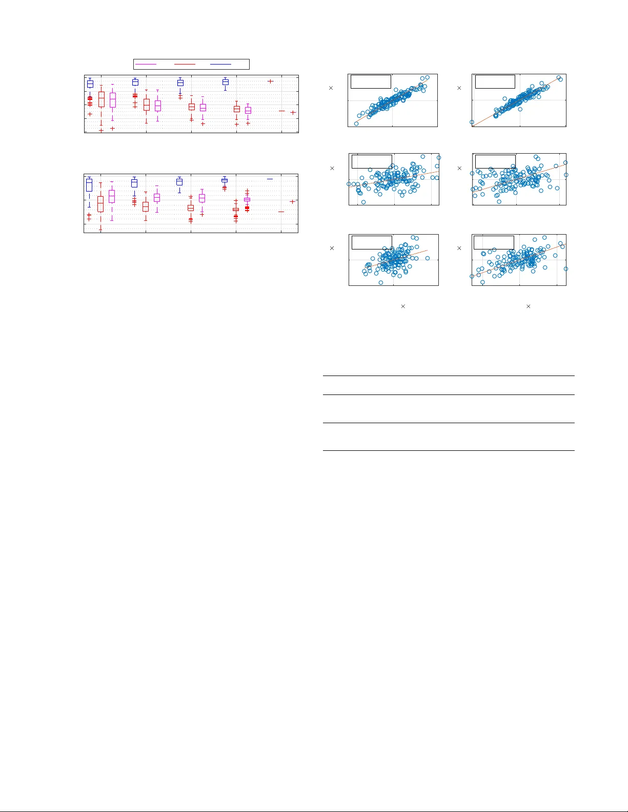
1 A T urv e y-Shaple y V alue Method for Distrib ution Network Cost Allocation Donald Azuatalam, Graduate Student Member , IEEE, Archie C. Chapman, Member , IEEE, and Gregor V erbi ˇ c, Senior Member , IEEE Abstract —This paper proposes a novel cost-reflective and com- putationally efficient method for allocating distrib ution network costs to residential customers. First, the method estimates the gro wth in peak demand with a 50% probability of exceedance (50POE) and the associated network augmentation costs using a probabilistic long-run marginal cost computation based on the T urvey perturbation method. Second, it allocates these costs to customers on a cost-causal basis using the Shapley value solution concept. T o over come the intractability of the exact Shapley value computation for r eal-world applications, we implement a fast, scalable and efficient clustering technique based on customers’ peak demand contribution, which drastically reduces the Shapley value computation time. Using customer load traces from an A ustralian smart grid trial ( Solar Home Electricity Data ), we demonstrate the efficacy of our method by comparing it with established energy- and peak demand-based cost allocation approaches. Index T erms —T urvey perturbation method, long-run marginal cost, Shapley value, k-means clustering, cost-causality , demand- based tariffs, cost-reflectiv e network pricing I . I N T RO D U C T I O N The rapid rise in the penetration lev els of distributed energy resources in low-v oltage distribution networks necessitates the design of network tariffs that allocate associated network costs in an ef ficient, fair and equitable manner to network users. Hence, distrib ution network service providers (DNSPs) and regulators in most jurisdictions are challenged with the tasks of designing efficient tariffs that are reflective of network cost dri vers [1]. Recent studies in this area have explored different methods for distribution network pricing, including transmission network pricing methodologies, such as Loca- tional Marginal Pricing (LMP), P osta ge Stamp (PS), MW- Mile , MV A-Mile , A verage P articipation (AP), and Mar ginal P articipation (MP) [2 – 6], Ramsey-Boiteux pricing , cooper- ative game theory or other extemporaneous cost allocation methodologies. Howe ver , in order to establish the performance of these methods with respect to established tariff design principles [7], which includes cost reflectiveness , efficiency , stability and fairness , we need to define a measure (bench- mark) of overall performance, with which to compare existing methods. T o this end, the purpose of our study is to use a principled cost allocation method as a performance benchmark for other allocation methodologies. Donald Azuatalam, Archie C. Chapman and Gregor V erbi ˇ c, are with the School of Electrical and Information Engineering, The Univ ersity of Sydney , Sydney , New South W ales, Australia. E- mail: donald.azuatalam@sydney .edu.au, archie.chapman@sydney .edu.au, gregor .v erbic@sydney .edu.au. Distribution network costs typically comprises three ma- jor cost components–energy costs, long-run marginal cost (LRMC), and residual (such as retail charges) costs. In order to adequately recover these cost components, network tariffs should be structured such that the fixed, energy and/or demand charges efficiently send the right price signals to customers to respond appropriately . For example, [8] used a three-part tariff for distribution network cost allocation. Here, the residual costs ($/day) were recovered through Ramsey pricing , while the LRMC ($/kW) and energy costs ($/kWh) were recov ered through coincident peak pricing and distribution locational mar ginal pricing (DLMP) respectively . Nev ertheless, network tariffs historically only consisted of energy-based (volumetric) and residual charges due to two reasons: (i) there w as little need to signal the LRMCs be- cause loads per feeder were relativ ely flat and (ii) pricing mechanisms available to utilities were sev erely constrained by metering technology . Ho wev er , with the introduction of smart meters, it is possible to implement tariffs which reflect congestion costs that driv es network in vestments. As such, network tariffs should be based on customers demand at network peak [8–13]. It should be time- and location-specific and should account for network losses and actual customer energy use. Additionally , a fair and equitable tariff should also eliminate or reduce inter-customer subsidies created due to PV owners, while safeguarding vulnerable customers [14, 15]. Unlike volumetric tariffs, peak demand-based tariffs are robust to technological changes (such as solar PV , EV or battery storage) which reshapes customers’ demand profiles while effecti vely signalling peak demand costs to customers [15, 16]. Thus, residual and/or LRMC costs can be recovered partly through demand-charges instead of constantly increas- ing fixed or energy charges for all customers [6, 17]. So far , coincident peak pricing (CPP) and critical peak pricing hav e been proposed to mitigate the impacts of DER on the equity of network cost allocations. Although peak demand-based tariffs are more complex than energy-based tarif fs, they can better allocate network costs on a cost-causal basis and ensure a stable revenue for network companies [15, 17]. Furthermore, [18] showed that customer bill volatility reduces with demand- based tariffs compared to real time pricing and time-of-use tariffs . Contrarily , [12] tested demand-based tariffs proposed by the Australian Energy Regulator (AER) on households in Sydney . It was concluded that without due adjustments made, these tariffs are low in cost-reflectivity . Generally , the suitability of network tarif fs in terms of fairness and cost- reflectivity depends on the assumptions made in the tariff 2 design and on customers’ price response [19]. This further highlights the need for a principled cost allocation benchmark. Further still, the distribution network tariff design problem encompasses more than the aforementioned requirements. Be- yond these, there are other three salient tariff design questions that need to be answered in order to achiev e a cost-reflective pricing and appropriate customer response: (i) What LRMC calculation method should be used – the T urve y perturbation method or the A verag e Incr emental Cost method ? (ii) What peak demand should be the basis for charging customers – indi vidual customer peak, distrib ution network coincident peak or zone-substation peak? and, (iii) What is the optimal frequency of peak demand measurement – monthly or yearly basis? [17]. The answers to these questions form the basis for practically implementing tariffs that better recuperate forward- looking network costs. Ho we ver , there are no clear -cut answers to these questions, because choices for network companies depend on other factors, such as customer socio-demographics, customer class, and the av ailability of smart meters and energy management systems. Nonetheless, recent research in the area argues that demand-based tariffs should be based on network coincident peak since it better signals LRMC. Ho wev er , in practice, customers’ coincident peak demand is hard to mea- sure and thus CPP is dif ficult to implement. Thus, demand charges are a step-forward to attaining optimal network tariffs. In this paper, we seek, based on established economic prin- ciples, to make a further step tow ards the design of equitable network pricing. Our focus is to provide a measure for the fair and efficient allocation of costs that signal the drivers of future network in vestment. T o achiev e this, we dev elop a nov el method to apportion the LRMC, using a probabilistic approach to the T urve y perturbation method ([20]) linked via the characteristic function of a cooperativ e game 1 to the Shaple y value (SV) cost allocation rule [21, 22]. In more detail, the T urve y perturbation method is a forward- looking and more time- and location-specific method for LRMC estimation, compared to the simpler av erage incre- mental cost methods widely used by network companies [17]. Furthermore, [23, 24] argue that the T urvey perturbation method is the preferred option since it better aligns with the underpinning principles gov erning LRMC. Howe ver , research in [25] concluded that both methods can be equally used for LRMC calculations. At the same time, the SV gives a vector-v alued solution to a cooperativ e transferable utility (TU) game, where the total cost or worth of a coalition is defined by a single-valued char- acteristic function . In our method, the characteristic function is the probabilistic LRMC defined using the Turv ey perturbation method. The SV has found several applications including con- sumer demand response compensation [26 – 28], transmission network cost allocation [29–31], distribution network loss allo- cation [32], and other cost allocation problems [26, 27, 33 – 35]. Howe v er , due to the computational complexity of computing the exact SV for a large number of players, it’ s application is usually limited to small problems. Recent research in this area, 1 A cooperativ e game models a game where a group of players cooperate to earn a joint reward, which has to be shared among the players in a fair and stable way . nonetheless, has seen dev elopments of approximate methods of calculating the SV in polynomial time [27, 34 – 39]. In [27], a comparison of the accuracy and scalability of two approximate SV computation algorithms was made, namely linear-time appr oximation [36] and stratified sampling [39, 40] techniques. While the stratified sampling approach was more accurate, the linear-time appr oximation required less memory and computation time as the number of players increased. This is a general finding, so with these methods, there is always a trade-off between accuracy and computational complexity . Moreov er , some of these methods are only suited to weighted voting games , which does not match our cost-allocation prob- lem. In a different research direction, a clustering approach was adopted in [38], where customers are segmented into major classes. Howe v er , customers in the same class are assigned the same SV . Con v ersely , for distribution netw ork cost allocation, this is not the case, as the SV should be different for all customers. In light of these shortcomings, we deriv e a computationally- efficient clustering algorithm, to allocate network costs based on the T urvey-Shaple y v alue method. The SV is computed at the lev el of clusters, and individual customers are allotted a portion of this SV based on their av erage coincident peak demand contribution to each coalition of their representativ e cluster . This approximation approach is validated by compar- ison to the exact SV calculation, for which the SV estimation error is shown to be small and reduces as the number of customers increases (i.e. when approximation become com- putationally necessary). Furthermore, as the SV method best allocates network costs in a principled, fair and stable manner , we used it as a benchmark to measure the cost-reflectivity of other cost allocation methodologies. In summary , the analysis in this paper extends the preliminary results in our earlier conference paper [41] in the following ways: • W e propose a probabilistic approach to the Turv ey LRMC computation via a W eibull distribution, which giv es an unbiased estimate of forward-looking network costs. • W e propose a peak load contribution clustering technique interleav ed with the T urvey-Shaple y value method to com- pute the Shapley value for large number of customers with low computation time and estimation error . • W e demonstrate the effecti veness of our methodology using real customer load traces from the Solar Home Electricity Data 2 . Our results show that the proposed allocation method is the most reflectiv e of network capacity costs compared to other cost allocation methodologies. The remainder of this paper is structured as follows. Section II provides preliminaries on cooperativ e game theory and the Shapley value. In Section III, we describe the methodology , including the Turv ey pricing method. The results are presented and discussed in Section IV. Section V concludes. I I . P R E L I M I NA R I E S In this section, we provide a background to cooperativ e games, the Shaple y value and its characteristics, and the T urvey perturbation method . 2 Dataset is av ailable at https://data.nsw .go v .au/ 3 A. Cooperative Games Formally , we consider the class of transferable utility (TU) games, which are cooperative games that allo w the transfer of worths between players. If the players in a cooperative game agree to work together, they form a coalition . If all n players form a coalition, it is called the grand coalition . Each player incurs some priv ate cost in completing its component of the joint action, while collectiv ely , the joint action has some worth associated with it. Definition II.1. A TU game is giv en by Γ = hN , w i where: • N is a set of n players , and • w ( S ) is a char acteristic function , w : 2 n → < + with w ( ∅ ) = 0 , that maps from each possible coalition S ⊆ N to the worth of S . Before defining the Shapley value, we first formally define some important characteristics of any solution to a TU game. Definition II.2. Gi ven a Γ , a solution concept defines a worth to each player , which is a vector of transfers (worths), φ = ( φ 1 , . . . , φ i , . . . , φ n ) ∈ < n . W e denote the sum of worths as P i ∈S φ i = φ ( S ) . Some desirable properties of solutions concepts include the follow- ing; a solution is: • Efficient if φ ( S ) = w ( S ) , so that the worth vector exactly divides the coalitions worth, • Symmetric if φ i = φ j if w ( S ∪ { i } ) = w ( S ∪ { j } ) , ∀ S ⊆ N \ { i, j } . This means that equal worths are made to symmetric players, where symmetry means that we can ex- change one player for the other in any coalition that contains only one of the players and not change the coalition’ s worth. • Additive if for any two additiv e games the solution can be giv en by φ i ( v 1 + v 2 ) = φ i ( v 1 ) + φ i ( v 2 ) for all players. That is, an additive solution assigns worths to the players in the combined game that are the sum of their worths in the two individual games. • Zer o worth to a null player if a player i that contributes nothing to any coalition, such that w ( S ∪ { i } ) = w ( S ) for all S , then the player receives a worth of 0. B. The Shaple y V alue (SV) Solution concepts in cooperativ e game theory define divi- sions of the group reward among players, while considering the rewards av ailable to each alternative coalition of players. The SV is one of such solution concepts which also satisfies the desirable properties listed above, by virtue of its definition. Definition II.3. The SV allocates to player i in a coalitional game h w , N i the worth: φ i ( w ) = 1 n X S ⊆N \ i  n − 1 |S |  − 1 ( w ( S ∪ { i } ) − w ( S )) (1) Here, the vector -v alued function φ has the follo wing in- tuitiv e interpretation: consider a coalition being formed by adding one player at a time. When i joins the coalition S , its mar ginal worth is gi ven by w ( S ∪ { i } ) − w ( S ) . Then, for each player , its SV worth is the average of its marginal Algorithm 1 Exact Turv ey-Shaple y V alue Algorithm ( Exact ) N : set of players/customers, N = { 1 , .., n } L : set of all coalitions, L = {S 1 , .., S l , ..., S 2 n − 1 } 1: for each customer i ∈ N do 2: for each coalition S ∈ L : i ∈ S do 3: µ = 50POE yearly peak demand of S 4: Find X ∼ W ( α, β ) of µ exceeding line limit x 5: α = µ/ Γ(1 + 1 /β ) with β = 1 . 5 6: if P ( X ≥ x ) < 0 . 001 then 7: w ( S ) = P ( X ≥ x ) Y 8: else 9: w ( S ) = 0 10: end if 11: Compute M S i = w ( S ) − w ( S − { i } ) 12: Compute K S i = (1 /n !)( |S | − 1)! ( n − |S | )! 13: end for 14: Return SV of i , φ i ( w ) = P S ∈L K S i M S i 15: end for contributions over the possible dif ferent orders in which the coalition can be formed. The expression in (1) can also be interpreted as a player’ s contribution to all subsets of N that do not contain it, where the binomial term is the number of coalitions of size |S | . W e can further expand this expression to identify a useful approximation. Specifically , the summation in (1) can be expressed in terms of the size of the coalitions that i is added to, as follows: φ i ( w ) = 1 n n − 1 X k =0    n − 1 k  − 1 X S ∈S k ( w ( S ∪ { i } ) − w ( S ))   (2) where: S k = {S ⊆ N \ i : |S | = k } is the set of coalitions of size k that exclude i . W e can now approach the SV by approximating the inner term for each size k ∈ { 0 , . . . , n − 1 } . One approach is to statistically estimate the term: χ k =  n − 1 k  − 1 X S ∈S k ( w ( S ∪ { i } ) − w ( S )) (3) using a sample-based approach. This is a randomised sampling algorithm described in detail in Section III-C. C. The T urve y P erturbation Method The T urve y perturbation method [20] is one technique used to estimate the LRMC of capacity-based inv estments. It quantifies the effects of a (small) permanent change in demand Q on future capital costs C . It is defined in [25] as: T urve y LRMC = P V (∆ C ) P V (∆ Q ) (4) The expression in (4) translates to–the ratio of the present value of change in costs (due to a permanent change in demand) to the present value of the permanent change in demand. The T urvey perturbation method therefore in volves forecasting demand over the estimation period, with a certain confidence lev el. For this, we assume a small growth in yearly peak demand with a 50% probability of exceedance. As explained in detail in the next section, in our method- ology , the probability that this value exceeds the network 4 line limit informs the LRMC. This probabilistic approach to the T urve y perturbation method, achiev ed via a W eibull distribution, is used to construct the characteristic function for the SV computation. I I I . M E T H O D O L O G Y In this section, we detail the steps taken to assess the cost- reflectivity in the allocation of distribution network tariffs to L V residential customers, with the SV allocation being the benchmark. First, we explain the T urve y-Shaple y value LRMC estimation and allocation methodology . Second, we describe algorithms to determine the exact SV for a set of customers N , and its approximation. The approximation algorithms are required to compute the SV for n > 25 players, with lower computational burden and minimal loss in accuracy . A. T urve y-Shaple y V alue LRMC Methodology The proposed T urvey-Shaple y value LRMC methodology in volv es interleaving of a novel probabilistic approach to the T urve y perturbation method with the SV characteristic function , and is illustrated in Algorithm 1. In this section, we explain the steps for the T urve y LRMC estimation and SV cost allocation. First, we calculate the line limit x of the given network with line augmentation cost Y . This is giv en as the yearly peak demand of the network (i.e. grand coalition of customers) multiplied by a factor of 1.5 (to account for distribution line emergenc y limit). W e have assumed that the probability of a coalition’ s 50 POE peak demand exceeding the line limit follows a W eibull distribution, X ∼ W ( α, β ) 3 . The two- parameter W eibull distribution function is defined as: F α,β ( x ) = 1 − exp h −  x α  β i for x ≥ 0 (5) where α > 0 is the scale parameter and β > 0 is the shape parameter . In order to obtain the standard fat-tailed W eib ull distribution that is required in this study , β is taken as 1.5. Then, for each coalition, we assume a yearly peak demand growth rate of 1% as the 50 POE value, which is taken as the mean µ of the W eibull distribution. Giv en the mean and shape factor , we calculate the scale factor of the distribution. If the tail probability P ( X ≥ x ) of a coalition’ s 50 POE peak demand exceeding the line limit is less than 0.001, we neglect the coalition cost (set as zero) in the incremental cost (IC) calculations for a particular customer in each coalition size. For example, if Y is $1M, then we neglect coalitions with cost less than $1k, which improves the incremental cost computation time of each customer . Otherwise, the coalition cost is giv en as P ( X ≥ x ) Y , that is, the coalition’ s expected LRMC under the corresponding W eibull distribution. The SV for each customer i ∈ N is calculated as the av erage of its marginal contributions to all coalitions containing i , as in (1). In the ne xt three subsections, we describe the exact SV algo- rithm ( Exact ), and two algorithms ( Sampling and Clustering ) to compute the approximate SV for up to 25 customers. 3 This choice is not essential to the method; any other fat-tailed distribution could be used as well. Algorithm 2 Randomised Sampling Algorithm ( Sampling ) N : set of players/customers, N = { 1 , ..., n } K : partition of set of k -sized coalitions, K = {S 1 , .., S k , .., S n } 1: for each customer i ∈ N do 2: for each set of k -sized coalitions S k ∈ K do 3: Find G ⊂ S k : ∀ Z ∈ G , i ∈ Z 4: if |S k | < 10000 then 5: for each coalition g ∈ G do 6: θ g = ( k − 1)! ( n − k )! n ! ( w ( g ) − w ( g − { i } )) 7: end for 8: ϑ S k = P g ∈G θ g 9: else 10: Sample |P | coalitions from |G | : |P | = K 11: for each coalition p ∈ P do 12: θ p = ( w ( p ) − w ( p − { i } )) 13: end for 14: Compute standard deviation σ P of all θ p ∈P 15: Compute optimal sample size, |P 0 | using (6) 16: Sample |P 0 | coalitions from |G | 17: for each coalition p 0 ∈ P 0 do 18: θ p 0 = ( k − 1)! ( n − k )! n ! ( w ( p 0 ) − w ( p 0 − { i } )) 19: end for 20: ϑ S k = P p 0 ∈P 0 θ p 0 21: end if 22: end for 23: φ i = P S k ∈K ϑ S k 24: end for B. Dir ect Enumeration The exact algorithm ( Exact ), also known as direct enumer- ation , is based on (1) and is described in Algorithm 1. In terms of computational speed, it performs well with n < 20 players. But with n > 25 , its performance (w .r .t. speed and memory requirements) deteriorates because of the time taken and memory required to compute the large ( 2 n − 1 ) × n coalition matrix. Note that Line 2 in Algorithm 1 can be broken down into n coalition sizes according to (2). C. Randomised Sampling As explained in Section II-B, we use a sample-based ran- domised algorithm which statistically estimates (3), to provide approximate SV calculations based on (2). W ith this, we do not perform all the incremental cost calculations ( 2 n − 1 ) required to compute the exact SV for each customer . Instead, we do this only for coalition sets that contain more than 10,000 possible coalitions of the same size. In Algorithm 2 ( Sampling ), we first select randomly a pilot sample ( |P | = K ) from such large coalitions, where K is determined by trial and error . Then, the standard deviation σ P of the marginal contribution of customer i to the sampled coalition is computed, followed by the calculation of the optimal sample size using: |P 0 | =  Z σ P d  2 (6) where Z = 1 . 96 is the z-score of 95% confidence in a Gaussian distribution and d = 0 . 2 is taken to be the margin of error for the sampling estimation. D. Clustering Method The clustering method illustrated in Algorithm 3 is also based on (2). In this method, we first cluster |H m | = 125 5 Algorithm 3 Clustering Algorithm ( Clustering ) H : partition of set of network users, H := {H 1 , .., H h , .., H m } N : set of players/clusters, N = { 1 , ..., n } K : partition of set of k -sized coalitions, K = {S 1 , .., S k , .., S n } 1: Cluster |H m | customers into n clusters 2: for each H h ∈ H do 3: for t ← − 1 to 100 step 1 do  100 MC simulations 4: Sample |H h | customers uniformly from |H m | 5: for each cluster i ∈ N do 6: for each set of k -sized coalitions S k ∈ K do 7: Find G ⊂ S k : ∀ Z ∈ G , i ∈ Z 8: for each coalition g ∈ G do 9: Find H h i ⊂ H h  customers in cluster i 10: V H h i g = [ v 1 g , ..., v |H h i | g ]  cust. contr . to w ( g ) 11: θ g = ( k − 1)! ( n − k )! n ! ( w ( g ) − w ( g − { i } )) 12: end for 13: ϑ S k = P g ∈G θ g 14: end for 15: φ i = P S k ∈K ϑ S k  SV of cluster i 16: φ H h i t = ( φ i / |G | ) P g ∈G V H h i g  SV –customers in i 17: end for 18: end for 19: end for customers from the Ausgrid Solar Home Electricity Data set into n = 5 representativ e load profile clusters (with minimum customer set |H 1 | = 25 ). Here, end-users are clustered based on their half-hourly av erage daily consumption pattern for a year using the k-means clustering algorithm. Next, for each set of network users H h ∈ H , we find the yearly demand (with 30-minute resolution) of each cluster i ∈ N , by summing the half-hourly demand of all customers belonging to cluster i . Then, we find the average contribution V H h i g of member customers to the yearly peak demand of cluster i ov er all coalitions g ∈ G . After computing the SV of each cluster , the cluster cost is then apportioned to its member customers according to their contribution. It is worth noting that the algorithm can be scaled to compute the SV for |H m | > 125 network users in our dataset, with just an insignificant clustering ov erhead computation cost for allocating customers into 5 clusters; and moreov er , it would scale to settings with up to 25 clusters irrespectiv e of the total number of customers. . I V . C A S E S T U D Y , R E S U LT S A N D D I S C U S S I O N In this section, we assess the computational performance and accurac y of the SV approximation methods, the correlation of SV with three peak demand indicators commonly used to define tarif fs, and compare alternativ e pricing methods with the SV cost allocation. T o begin, we define the following three peak demand indicators as follows: • Coincident peak demand (CPD): This refers to a customer’ s coincident peak demand at the time of the network’ s yearly peak load. • Individual peak demand (IPD): This refers to a customer’ s yearly peak demand. • T otal peak demand (TPD): This refers to the sum total of a customer’ s monthly peak demand values in a year . 5 10 15 20 25 Number of customers 10 -2 10 0 10 2 SV computation time (min) Exact Sampling Clustering (a) Sampling Clustering SV approximation 10 -5 10 -4 10 -3 10 -2 RMSE 5 10 15 20 25 (b) Fig. 1: (a) SV computation time for 5 – 25 customers (b) Error in approximate SV calculation for 5 – 25 customers. For both plots, the y-axis is in log scale. T ABLE I: Network T ariff Data T ariff T ype Fixed charge c / day Anytime Energy c / kWh Off peak Energy c / kWh Shoulder Energy c / kWh Peak Energy c / kWh Flat 40.097 11.163 - - - T oU 40.097 - 2.805 7.086 27.335 As case study , the net load traces (solar PV and demand) used in this work were sourced from the Ausgrid (DNSP in NSW) Solar Home Electricity Data . The dataset comprises three years of half-hourly resolution smart meter data for the period between July 2010 to June 2013, for 300 residential customers in the Sydney region of Australia. Howe ver , we could only extract 125 customers from this dataset with complete solar PV and demand data, for the period between July 2012 to June 2013. This information is used to obtain the abov e defined peak demand indicators for each customer . W e also employ network tariff data from Ausgrid 4 , giv en in T able I 5 , which enables us make a rough estimate of the rev enue obtained for these customers under the flat and T oU energy network prices. A. SV Computation T ime and Accuracy Here, we compare the computational performance and accu- racy of the dif ferent SV calculation algorithms. F or this first set of computations, we have assumed that all customers possess solar PV , so the net load is used to compute their monthly peak demand. Fig. 1a shows the SV computation time in minutes for all customer sizes from 5 up to 25 users. A related point to consider is that the exact SV computation for more than 25 users is not computationally feasible. The Exact algorithm performs best for n < 15 customers, but with n ≥ 15 , this 4 Ausgrid Network Price List. A vailable at https://www .ausgrid.com.au/Industry/Re gulation/Network-prices. 5 Peak: summer weekdays (Nov . to Mar.) between 2pm to 8pm, winter weekdays (Jun. to Aug.) between 5pm to 9pm; Shoulder: weekdays year round, between 7am to 10pm (exc. Peak periods); Off-peak: all other times. 6 25 50 75 100 125 0.2 0.4 0.6 0.8 1 Linear Correlation TPD IPD CPD (a) W ithout PV 25 50 75 100 125 Number of Customers 0 0.5 1 Linear Correlation (b) W ith PV Fig. 2: SV linear correlation coefficient box plot. CPD–coincident peak demand, IPD–individual peak demand, TPD–total peak demand. Note that there is no statistical variance for n = 125 . is not the case. It takes 418 minutes to compute the SV for n = 25 customers, due to the time and memory consuming coalition matrix generation and the corresponding coalition cost function calculations. Con versely , there is a significant improvement in computa- tional performance with the first approximate algorithm com- pared to Exact . Sampling tak es only 98 minutes to compute the SV for n = 25 (about a quarter of the time taken for Exact ). This reduction in computation time is as a result of performing IC calculations for a select (optimal) sample, using a constant number as a pilot sampling size, instead of performing the IC calculations for all coalitions (in Exact ) at the same time. Furthermore, splitting the total coalitions into n coalition sizes in Sampling overcomes the memory limitations of Exact . On the other hand, the clustering algorithm takes the least time to compute the SV for n ≥ 15 customers. This is because the SV calculation is done for only 5 players (or clusters), with a little overhead computation cost for clustering. T o ev aluate the accuracy of the sampling and the clustering technique, we find the root mean square error (RMSE) in the SV estimation. Fig. 1b shows RMSE values between 10 − 2 and 10 − 5 relativ e to mean values between 0 . 04 and 0 . 2 for n ≤ 25 customers. Although the sampling approach is more accurate than the clustering technique for 5 < n ≤ 25 , it cannot be up-scaled to n > 25 players, without a significant increase in the computation time. Besides, with the clustering technique, the estimation error reduces as more customers are added to make the clusters more representativ e. B. SV Linear Correlation with P eak demand Indicators This section shows the results obtained by finding the linear correlation between the SV computed using the clustering technique and the peak demand indicators, for two scenarios (i) all customers without PV and (ii) all customers with PV . Since the SV is computed for 100 Monte Carlo runs based on uniform random sampling, the Pearson’ s correlation 6 8 10 6 8 10 Norm. CPD 10 -3 R = 0.948 7 8 9 7 8 9 Norm. CPD 10 -3 R = 0.947 7.5 8 8.5 6 8 10 Norm. IPD 10 -3 R = 0.507 7.5 8 8.5 7 8 9 Norm. IPD 10 -3 R = 0.249 7 8 9 Norm. SV 10 -3 6 8 10 Norm. TPD 10 -3 R = 0.485 (a) W ithout PV 7.5 8 8.5 Norm. SV 10 -3 7 8 9 Norm. TPD 10 -3 R = 0.468 (b) W ith PV Fig. 3: SV linear correlation scatter plot for 125 customers. CPD–coincident peak demand, IPD–individual peak demand, TPD–total peak demand. T ABLE II: Mean SV correlation with Peak demand Indicators Scenario Peak demand Indicator Customers 25 50 75 100 125 W ithout PV Coincident 0.8773 0.9134 0.9114 0.9272 0.9478 Individual 0.6668 0.5891 0.5644 0.5321 0.5065 T otal 0.6626 0.5833 0.5541 0.5140 0.4848 W ith PV Coincident 0.7967 0.8380 0.8780 0.9098 0.9473 Individual 0.4113 0.3625 0.3291 0.2918 0.2493 T otal 0.5700 0.5512 0.5277 0.5016 0.4685 coefficients (R-v alue) are presented as box plots in Fig. 2 while T able II shows the mean values, for H of size 25, 50, 75, 100, and 125. For Scenario 1 (Fig. 2a), the SV correlates more with Individual peak demand than with T otal peak demand but for Scenario 2 (Fig. 2b), the con v erse is the case. It is w orth noting that Individual and T otal corresponds to charging customers based on their yearly peak load and monthly peak load re- spectiv ely . W ithout PV , a customer’ s true demand is rev ealed, which is less sensitiv e to weather, so individual peak demand dominates. Howe ver , with PV , a customer’ s demand profile is modified with PV generation which is season-dependent, and as such it’ s better to charge customers on a monthly basis. Nev ertheless, for both scenarios, the SV correlates most with Coincident peak demand, because it driv es augmentation cost the most. Figs. 3a and 3b sho w the scatter plot for SV correlation with the peak demand indicators for n = 125 customers without PV and with PV respectively . For Scenario 1, the mean R-values are 0.948, 0.507 and 0.485, for Coincident , Individual , and T otal peak demand respectively while the R-values for Scenario 2 are 0.947, 0.249 and 0.468, for Coincident , Individual , and T otal peak demand respectiv ely . 7 Flat ToU CP YP MP SV 0 0.5 1 Linear Correlation CPD IPD TPD Flat ToU CP YP MP SV 0 0.5 1 EB CP YP MP 10 1 10 2 RMSE Flat Revenue ToU Revenue (a) W ithout PV EB CP YP MP 10 2 Flat Revenue ToU Revenue (b) W ith PV Fig. 4: (a) Correlation between cost allocation method and peak demand variants (top) and error in cost allocation from the SV allocation (bottom). EB–energy-based, CP–coincident peak, YP–yearly peak, MP–monthly peak. While CPD and TPD have similar v alues in both scenarios, IPD is considerably different. This is because a customer’ s (individual) yearly peak demand changes significantly with the addition of PV . C. Comparison of Cost Allocation Methodologies Here, we ev aluate ho w dif ferent energy-based and peak demand-based cost allocation methodologies compare to the SV , by measuring the correlation between normalised cus- tomer cost allocation and specifically-defined peak demand indicators. First, we perform the SV computation for n = 125 customers, for both scenarios. Then, we estimate the rev enue obtained by the DNSP for these customers under the two tariffs (Flat- and T oU-based) described in Section III. For this, we hav e hav e neglected the feed-in-tariff (FiT) as it is administered through a different mechanism and handled by retailers in the Australian electricity system’ s regulatory and billing arrangements. Therefore, we use only the power import from the grid for our calculations. W e consider the following cost allocation methods in our analysis: • Energy-based (EB - Flat or T oU) • Coincident peak load (CP - Coincident peak) • Y early peak load (YP - Individual peak) • Monthly peak load (MP - T otal peak) and • Shapley value cost allocation (SV) In the first method, cost allocation is done according to the rev enue calculations under Flat and T oU tariff for n = 125 customers, using tariff values in T able I. For the rest, we split the total rev enue obtained using the energy-based tariffs, ac- cording to the normalised SV and the normalised Coincident , Individual , and T otal peak demand values for each customer . The top part of Fig. 4 shows the correlation between the different cost allocation methodologies and the peak demand indicators. From these, we can deduce that the SV provides a fine balance between coincident, individual and aggregate peak demand, since it properly accounts for network usage at times other than the coincident network peak. This is by virtue of the way it is being computed, by ev aluating the marginal contribution of customers to all possible coalitions. Although, the major cost dri ver for distrib ution networks is the coincident peak demand, it is necessary for a cost-reflectiv e tariff design to appropriately account for aggregate and indi vidual customer peak demand. Furthermore, the yearly and monthly peak de- mand allocation are also not cost-reflective, since they have a lower correlation with coincident peak demand compared with the SV allocation. Energy-based allocation methods perform worst as they show much lower correlation with the peak demand indicators. Howe ver , the results for Scenario 2 show that T oU-energy based allocation is better than that of Flat- energy based allocation as it shows comparativ ely higher R- values. Moreov er , these results implicitly show that inter- customer subsidies will be reduced since customers would be paying their fair share, given the similar R-value for Coincident peak demand in both scenarios. At the bottom part of Fig. 4, we sho w the error (RMSE) in actual cost values that will arise when a DNSP allocates cost to customers using less optimal cost allocation methodologies. This translates to inaccurate wealth transfer amongst cus- tomers in a distribution network. As expected, there are higher RMSE v alues resulting from energy-based cost allocation methods. This implies that they are least cost-reflective for both scenarios, both in terms of cost-causality and equity in cost allocation. Also, for both scenarios, the coincident peak load allocation results in the least error because the main cost driv er for networks is the coincident peak. While the monthly peak allocation, and the yearly peak demand allocation method results in similar RMSE values for Scenario 1, this is not the case for the second scenario. When all customers possess PV , the monthly peak allocation results in slightly lower RMSE compared to the yearly peak demand allocation. This sho ws that for residential customers with PV , using a monthly peak demand network tariff is more cost reflective than a yearly peak demand tariff. It will be unfair to charge customers based on their sole highest yearly peak demand, which occurs in just one month of a year, and does not account for the seasonality in energy consumption which comes with PV generation. V . C O N C L U S I O N S A N D F U T U R E W O R K In this work, we showed the efficac y of the T urve y-Shaple y value method in calculating and apportioning LRMC to net- work users in a cost-reflecti ve way and with lo w computational burden using the proposed clustering technique. W e hav e demonstrated that the SV is a cost-reflective cost allocation method for networks with a large number of customers, regardless of PV adoption. This is because the SV is a principled technique, which provides a proper balance between the peak demand indicators (network cost driv ers). This makes for a fair cost allocation, which further reduces inter-customer subsidies. Other peak demand-based cost allo- cation approaches perform well up to the extent to which they appropriately balance the peak demand indicators, but with a greater emphasis on coincident peak demand. Furthermore, our results show that energy-based cost allocation methodologies are least cost-reflective as they least correlate with the peak demand indicators. 8 For future work, we will consider LRMC allocation for cus- tomers with both PV and batteries. In this case, an optimisation would hav e to be solved for each cost function computation. R E F E R E N C E S [1] A. Picciariello, J. Reneses, P . Frias, and L. S ¨ oder , “Distributed generation and distribution pricing: Why do we need new tariff design methodologies?” Electric P ower Systems Resear ch , vol. 119, pp. 370–376, 2015. [2] F . J. Rubio-Od ´ eriz and I. J. Perez-Arriaga, “Marginal pricing of transmission services: A comparativ e analysis of network cost allocation methods, ” IEEE T r ans. P ower Systems , vol. 15, no. 1, pp. 448–454, 2000. [3] J. Zolezzi, H. Rudnick, F . Danitz, J. Bialek, J. Pan, Y . T eklu, S. Rahman, and K. Jun, “Revie w of usage-based transmission cost allocation methods under open access [discussion], ” IEEE T r ans. P ower Systems , vol. 16, no. 4, pp. 933–934, 2001. [4] P . M. Sotkiewicz and J. M. V ignolo, “ Allocation of fixed costs in distribution networks with distributed generation, ” IEEE T rans. P ower Systems , vol. 21, no. 2, pp. 639–652, 2006. [5] F . Li, N. P . Padhy , J. W ang, and B. Kuri, “Cost-benefit reflecti ve distribution charging methodology , ” IEEE T r ans. P ower Sys- tems , vol. 23, no. 1, pp. 58–64, 2008. [6] T . Brown, A. Faruqui, and L. Grausz, “Efficient tariff struc- tures for distribution network services, ” Economic Analysis and P olicy , vol. 48, pp. 139–149, 2015. [7] J. C. Bonbright, A. L. Danielsen, and D. R. Kamerschen, Principles of public utility rates . Columbia Univ ersity Press New Y ork, 1961. [8] I. Abdelmotteleb, T . G ´ omez, J. P . C. ´ Avila, and J. Reneses, “Designing efficient distribution network charges in the context of activ e customers, ” Applied Energy , vol. 210, pp. 815–826, 2018. [9] W . A. Lewis, “The two-part tariff, ” Economica , vol. 8, no. 31, pp. 249–270, 1941. [10] M. P . Boiteux and P . Stasi, “Sur la d ´ etermination des prix de revient de d ´ eveloppement dans un syst ´ eme interconnect ´ e de production-distribution, ” International Union of Producers and Distributors of Electrical Ener gy (UNIPEDE), T ech. Rep., 1952. [11] M. Nijhuis, M. Gibescu, and J. Cobben, “ Analysis of reflectiv- ity & predictability of electricity network tariff structures for household consumers, ” Energy P olicy , vol. 109, pp. 631–641, 2017. [12] R. Passey , N. Haghdadi, A. Bruce, and I. MacGill, “Designing more cost reflectiv e electricity network tariffs with demand charges, ” Energy P olicy , vol. 109, pp. 642–649, 2017. [13] T . Nelson and F . Orton, “ A new approach to congestion pricing in electricity markets: Improving user pays pricing incentiv es, ” Ener gy Economics , vol. 40, pp. 1–7, 2013. [14] A. Picciariello, C. V ergara, J. Reneses, P . Fr ´ ıas, and L. S ¨ oder , “Electricity distribution tarif fs and distributed generation: Quan- tifying cross-subsidies from consumers to prosumers, ” Utilities P olicy , vol. 37, pp. 23–33, 2015. [15] P . Simshauser, “Network tariffs: resolving rate instability and hidden subsidies, ” W orking paper 45, AGL Applied Economic and P olicy Resear ch , 2014. [16] A. J. Pimm, T . T . Cockerill, and P . G. T aylor , “T ime-of-use and time-of-export tariffs for home batteries: Effects on low voltage distribution networks, ” Journal of Energy Storage , vol. 18, pp. 447–458, 2018. [17] A. Faruqui, “Pricing directions: A stakeholder perspectiv e, ” Submission in response to the NSW DNSPs 2019-24 regulatory proposals and AER issues paper , T ech. Rep., 2018. [18] ——, “Rate design 3.0 – future of rate design, ” Public Utilities F ortnightly , May 2018. [19] K. Stenner , E. Frederiks, E. V . Hobman, and S. Meikle, “ Aus- tralian consumers’ likely response to cost-reflectiv e electricity pricing, ” CSIR O Australia, 2015. [20] R. Turv ey , “Marginal cost, ” The Economic Journal , vol. 79, no. 314, pp. 282–299, 1969. [21] L. S. Shapley , “ A value for n-person games, ” in Contributions to the Theory of Games , H. W . Kuhn and A. W . Tuck er , Eds. Princeton Univ ersity Press, 1953, vol. 28, pp. 307–317. [22] G. Chalkiadakis, E. Elkind, and M. W ooldridge, Computational Aspects of Cooperative Game Theory (Synthesis Lectur es on Artificial Inetlligence and Machine Learning) , 1st ed. Morgan & Claypool Publishers, 2011. [23] D. Biggar , “An exploration of NERA ’ s proposed approach to estimating long-run marginal cost, ” Sapere Research Group Limited, T ech. Rep., 27 January 2012. [24] NERA Economic Consulting, “Estimating Long Run Marginal Cost in the National Electricity Market – A Paper for the AEMC, ” AEMC, T ech. Rep., 19 December 2011. [25] R. T ooth, “Measuring long run marginal cost for pricing, ” Sapere Research Group Limited, T ech. Rep., March 2014. [26] G. O’Brien, A. El Gamal, and R. Rajagopal, “Shapley value estimation for compensation of participants in demand response programs, ” IEEE Tr ans. Smart Grid , vol. 6, no. 6, pp. 2837– 2844, 2015. [27] S. Bakr and S. Cranefield, “Using the Shapley V alue for Fair Consumer Compensation in Energy Demand Response Programs: Comparing Algorithms, ” in Data Science and Data Intensive Systems (DSDIS), 2015 IEEE International Confer- ence on . IEEE, 2015, pp. 440–447. [28] A. C. Chapman, S. Mhanna, and G. V erbi ˇ c, “Cooperativ e game theory for non-linear pricing of load-side distribution network support, ” in 2017 IREP Symposium Bulk P ower System Dynamics and Control , Aug 2017. [29] J. M. Zolezzi and H. Rudnick, “Transmission cost allocation by cooperativ e games and coalition formation, ” IEEE T r ans. P ower Systems , vol. 17, no. 4, pp. 1008–1015, 2002. [30] X. T an and T . Lie, “ Application of the Shapley value on transmission cost allocation in the competitiv e power market en vironment, ” IEE Pr oceedings-Generation, T ransmission and Distribution , vol. 149, no. 1, pp. 15–20, 2002. [31] S. Khare, B. Khan, and G. Agnihotri, “A Shapley value ap- proach for transmission usage cost allocation under contin- gent restructured market, ” in 2015 International Confer ence on Futuristic T r ends on Computational Analysis and Knowledge Management (ABLAZE) . IEEE, 2015, pp. 170–173. [32] S. Sharma and A. Abhyankar , “Loss allocation for weakly meshed distribution system using analytical formulation of Shapley value, ” IEEE T rans. P ower Systems , vol. 32, no. 2, pp. 1369–1377, 2017. [33] F . Ghassemi and V . Krishnamurthy , “ A cooperative game- theoretic measurement allocation algorithm for localization in unattended ground sensor networks, ” in 2008 11th International Confer ence on Information Fusion . IEEE, 2008. [34] R. Stanojevic, N. Laoutaris, and P . Rodriguez, “On economic heavy hitters: Shapley v alue analysis of 95th-percentile pricing, ” in Pr oceedings of the 10th ACM SIGCOMM conference on Internet measur ement . ACM, 2010, pp. 75–80. [35] S.-S. Byun, H. Moussavinik, and I. Balasingham, “Fair allo- cation of sensor measurements using shapley value, ” in IEEE 34th Conference on Local Computer Networks . IEEE, 2009, pp. 459–466. [36] S. S. Fatima, M. W ooldridge, and N. R. Jennings, “A linear approximation method for the Shapley value, ” Artificial Intelli- gence , vol. 172, no. 14, pp. 1673–1699, 2008. [37] ——, “A randomized method for the Shapley value for the voting game, ” in Pr oceedings of the 6th international joint confer ence on Autonomous agents and multiagent systems . A CM, 2007, p. 157. [38] L. David, O. Massol, and A. Moison, “The Shapley value as joint cost allocation mechanism: is the story definitely over, ” URL citeseerx. ist. psu. edu/viewdoc/summary , 2005. [39] J. Castro, D. G ´ omez, and J. T ejada, “Polynomial calculation of 9 the Shapley v alue based on sampling, ” Computers & Operations Resear ch , vol. 36, no. 5, pp. 1726–1730, 2009. [40] S. Maleki, L. T ran-Thanh, G. Hines, T . Rahwan, and A. Rogers, “Bounding the estimation error of sampling-based Shapley value approximation, ” arXiv pr eprint arXiv:1306.4265 , 2013. [41] D. Azuatalam, G. V erbi ˇ c, and A. Chapman, “Shapley value analysis of distribution network cost-causality pricing, ” in 2019 P owerT ech Confer ence, Milan . IEEE, 2019.