Nonlinear Dynamic Periodic Event-Triggered Control with Robustness to Packet Loss Based on Non-Monotonic Lyapunov Functions

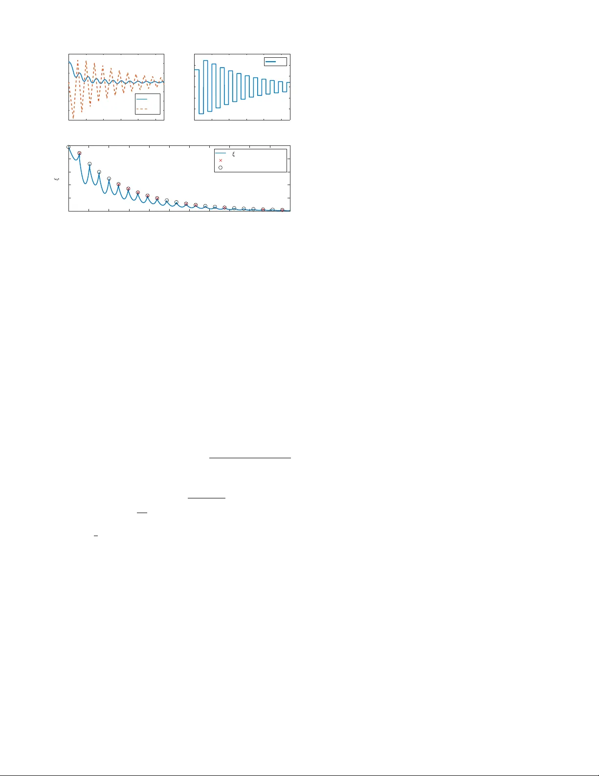
1 Nonlinear Dynamic P eriodic Event-T rigger ed Contr ol with Rob ustness to Pack et Loss Based on Non-Monotonic L yapunov Functions Michael Hertneck, Stef fen Linsenmayer , Frank Allg ¨ ower Abstract — This paper considers the stabilization of nonlinear continuous-time dynamical systems employing periodic event- triggered control (PETC). Assuming knowledge of a stabilizing feedback law for the continuous-time system with a certain con vergence rate, a dynamic, state dependent PETC mechanism is designed. The proposed mechanism guarantees on average the same worst case conv ergence behavior except f or tunable deviations. Furthermore, a new approach to determine the sam- pling period for the proposed PETC mechanism is presented. This appr oach as well as the actual trigger rule exploit the theory of non-monotonic L yapunov functions. An additional feature of the pr oposed PETC mechanism is the possibility to integrate knowledge about packet losses in the PETC design. The proposed PETC mechanism is illustrated with a nonlinear numerical example from literature. This paper is the accepted version of [1], containing also the proofs of the main results. I . I N T RO D U C T I O N Networked control systems (NCS) are control systems in which some or all links in the feedback loop are replaced by a shared communication network. Whilst NCS are useful in many modern control applications, several network induced problems have to be addressed (for a detailed overvie w see e.g. [2]). One major challenge in the field of NCS is the design of sampling and control strategies that use the network as little as possible to keep it av ailable for other applica- tions while being robust to unavoidable netw ork induced imperfections as e.g packet loss. Nevertheless, stability and performance goals like a certain conv ergence rate of the system state need to be guaranteed. A huge step towards tackling these two conflicting objectives was made by the dev elopment of event-triggered control (ETC) paradigms [3]. In ETC, control updates are sent over the network ac- cording to a system state dependent trigger rule. While classical results on ETC employ a static trigger rule [4], [5], in [6] the concept of dynamic ETC, where the trigger rule changes dynamically ov er time, has been introduced. Howe v er , ETC approaches like those in [4]-[6] require the continuous ev aluation of the trigger rule, which makes their implementation on digital platforms impossible. In periodic ev ent-triggered control (PETC) [7], [8], this problem is ov ercome by ev aluating the trigger rule only periodically at fixed sampling times. New information is transmitted at a sampling time if the trigger rule indicates it. Anyho w , whilst The authors thank the German Research Foundation (DFG) for support of this work within the German Excellence Strate gy under grant EXC-2075. The authors are with the Institute for Systems Theory and Auto- matic Control, University of Stuttgart, 70569 Stuttgart, Germany (email: { hertneck,linsenmayer ,allgower } @ist.uni-stuttgart.de). the number of transmissions can still be reduced in com- parison to time-triggered control, stability and performance guarantees from ETC are in general not preserved for PETC. Thus, it is desirable to find mechanisms tailored for PETC, such that stability , robustness to network imperfections and performance goals as a certain conv ergence rate of the system state can be guaranteed. Especially for nonlinear system dynamics, the design of such PETC mechanisms is a challenging task and deserves a comprehensi v e inv estigation. There exists a bunch of results considering PETC for linear systems, see e.g. [7], [8] for an ov erview . In dynamic PETC, a dynamically changing trigger rule is used like in dynamic ETC. In [9], dynamic PETC for linear systems with robustness to packet loss is in vestig ated. PETC results for nonlinear systems, either static or dynamic, are more rare. In [10], an ETC trigger rule is overapproximated to obtain a PETC trigger rule. In [11], [12], a PETC is emulated based on a stabilizing continuous-time controller . In [12], stability guarantees rely on the existence of a hybrid L yapunov function. For specific classes of nonlinear systems, PETC is in vestig ated in [13], [14]. In [15] it is shown, that ETC and PETC with a known (and chosen) conv ergence rate for nonlinear systems can be designed, provided that a control L yapuno v function is kno wn for the continuous-time system. Even though first results on PETC of nonlinear systems are av ailable, research is still at an early stage and it is thus de- sirable to find impro ved PETC mechanisms. It is furthermore worthwhile to prolongate the maximum admissible sampling period (MASP) of the PETC, which plays an important role for reducing the number of transmissions ov er the network. Also, the influence of network imperfections like packet loss on the PETC deserves a thorough in vestigation, in order to deal with aspects that arise in real world applications of NCS. In this paper, we present a novel dynamic trigger mecha- nism for PETC of nonlinear continuous-time systems that can guarantee stability and a chosen av eraged con ver gence rate if a controller and a L yapuno v function for the continuous- time system are kno wn. The proposed trigger mechanism is based on non-monotonic L yapuno v functions and can be viewed as a nonlinear counterpart to the dynamic trigger mechanism from [9]. It can be applied to a wide class of nonlinear systems and is robust to random packet loss if a bound on the number of successive lost packets is known. A lo wer bound on the MASP for the nov el trigger mecha- nism is constructed based on an extension of results from [15] considering non-monotonic L yapuno v functions [16] such that stability and a certain av eraged con ver gence rate c  2019 IEEE. Personal use of this material is permitted. Permission from IEEE must be obtained for all other uses, in any current or future media, including reprinting/republishing this material for advertising or promotional purposes, creating ne w collectiv e works, for resale or redistribution to serv ers or lists, or reuse of any copyrighted component of this work in other works. 2 (here indicated by a parameter σ ) can be guaranteed. This σ -MASP bound depends on lev el sets of the considered continuous-time L yapuno v function and is increased in most cases by factor 9 4 in comparison to the σ -MASP for the PETC from [15] while still guaranteeing the same av eraged worst case con ver gence rate except a time shift of ( m +1) sampling periods of the PETC, if the number of successi ve lost packets is bounded by m . This paper is the accepted version of [1], containing also the proofs of our main results. The remainder of this paper is structured as follows. The problem setup is described in Section II . Some basic results from [15] and [16] are recapped in Section III . The improv ed bound on the σ -MASP and the dynamic trigger mechanism are presented in Section IV . A numerical example to illus- trate the proposed PETC mechanism is giv en in Section V and Section VI concludes the paper . Some spacious proofs are gi ven in the Appendix. Notation: The positive (respectiv ely nonnegati ve) real numbers are denoted by R > 0 , respecti vely R ≥ 0 = R > 0 ∪ { 0 } . The positiv e (respectiv ely nonnegati ve) natural numbers are denoted by N , respectively N 0 := N ∪ { 0 } . A continuous function α : R ≥ 0 → R ≥ 0 is a class K function ,i.e., α ∈ K ), if α is strictly increasing and α (0) = 0 . The notation t − is used as t − := lim s 0 for all x 6 = 0 . V 0 ( k ) denotes ∂ V ( x ) ∂ x    x = k . Furthermore, we use in a slight abuse of notation L f V ( x, u ) to denote the Lie deriv ati v e of V along the vector field f : R n × R b → R n , i.e. L f V ( x, u ) = V 0 ( x ) f ( x, u ) . I I . P RO B L E M S E T U P In this section, we present the setup of this paper and formalize the control objective. A. Basic Setup W e consider a nonlinear , time-inv ariant system ˙ x = f ( x, u ) (1) with a smooth vector valued function f : R n × R b → R n satisfying f (0 , 0) = 0 , the system state x ( t ) ∈ R n with initial condition x (0) = x 0 and the input u ( t ) ∈ R b . The input is generated by u = κ ( ˆ x ) (2) with the nonlinear feedback law κ : R n → R b and a prediction ˆ x ( t ) of the system state x ( t ) that is generated at the actuator based on transmitted state information and ˆ x (0) = ˆ x 0 . The time instants, when state information is receiv ed by the actuator are giv en by the infinite sequence ( τ k ) k ∈ N 0 and define a discrete set T := { τ 0 , τ 1 , τ 2 , . . . } . The sequence T depends on a trigger mechanism, that will be designed in this paper, and on the capabilities of the communication network. Howe ver , we assume that current state information is receiv ed successfully at t = 0 and thus hav e τ 0 = 0 and ˆ x 0 = x 0 . The update of ˆ x at t ∈ T is represented by ˆ x ( t ) = x ( t ) . Between the update times, a state prediction can be designed based on the computational capabilities of the actuator as ˙ ˆ x ( t ) = f e ( ˆ x ( t )) , t / ∈ T (3) with f e (0) = 0 . If there are no computational capabilities, we can choose f e ( x ) = 0 , which corresponds to the zero order hold (ZOH) case. In this case, the next input ˆ u = κ ( x ) can be transmitted instead of the system state x even though we subsequently model the general case with ˆ x as a state. The closed-loop system combined of ( 1 ), controller ( 2 ), prediction ( 3 ) and its reset condition can be described as a discontinuous dynamical system (DDS) with state ξ =  ξ > 1 ξ > 2  > =  x > ˆ x >  > as ˙ ξ ( t ) =  f ( ξ 1 ( t ) , κ ( ξ 2 ( t ))) f e ( ξ 2 ( t ))  , t / ∈ T , ξ ( t ) =  I I  ξ 1 ( t − ) , t ∈ T \ { 0 } , (4) where ξ (0) =  x > 0 ˆ x > 0  > = ξ 0 . In order to design the PETC, we assume that a continuous-time feedback and a L yapuno v function are known, satisfying the following assumption. Assumption 1. (cf. [15]) There is a continuous, positiv e definite function V γ : R n → R , satisfying α 1 ( k x k ) ≤ V γ ( x ) ≤ α 2 ( k x k ) , (5) V 0 γ ( x ( t )) f ( x ( t ) , κ ( x ( t ))) ≤ − γ ( V γ ( x ( t ))) . (6) with class K functions γ , α 1 , α 2 . Finding κ and V γ that satisfy Assumption 1 is a fundamen- tal problem in control theory for continuous-time systems and is widely discussed in literature, see e.g. [17]. Thus we will not revie w it here in more detail. Subsequently , we consider local results for a le vel set of V γ , defined as X c := { x | V γ ( x ) ≤ c } for a chosen c ∈ R > 0 . B. Network Model and T rig gering Strate gy W e consider an unreliable network that can transmit pack- ets periodically with the sampling period h ∈ R > 0 . Network imperfections are modeled using the following assumption. Assumption 2. The consecuti ve number of lost packets is bounded by m ∈ N and there is an acknowledgment if a transmission was successful. This assumption allows random packet dropouts and re- quires no knowledge about the underlying probability dis- tribution as long as the boundedness condition is satisfied. It resembles the scenario where messages are dropped if they hav e a delay that is not negligible when the occurrence of such delays can be limited to a bounded number of successiv e transmissions. Necessary transmissions of the system state are detected using PETC, i.e. according to a trigger mechanism that is ev aluated at discrete, e v enly distributed time instants with the 3 sampling period h . The trigger rule of the PETC mechanism is thus ev aluated at sampling times t = z h for all z ∈ N 0 . If the trigger rule of the PETC mechanism is violated at a sampling time, a transmission of the system state is triggered. C. Con ver gence Criterion and Contr ol Objective A common con vergence criterion based on V γ and γ from Assumption 1 , that is used e.g. in [15], is d dt V γ ( x ( t )) ≤ − σ γ ( V γ ( x ( t ))) , ∀ t ≥ 0 (7) for some σ ∈ (0 , 1) . W e note that if ( 7 ) holds, then it holds due to the comparison Lemma [17, pp. 102-103] that V γ ( x ( t )) ≤ S ( t, x 0 ) , where S ( t, x 0 ) is the solution of d dt S ( t, x 0 ) = − σ γ ( S ( t, x 0 )) , S (0 , x 0 ) = V γ ( x 0 ) . (8) Thus S ( t, x 0 ) describes the worst case conv ergence behavior for ( 7 ) and can be used as a con vergence criterion as e.g. dis- cussed in [5], where an ETC is designed with a performance barrier based on S ( t, x 0 ) . For our PETC mechanism, we use an averaged criterion similar to ( 7 ) that can be described as V γ ( x ( t + ( m + 1) h )) ≤ S ( t, x 0 ) ∀ t ≥ 0 . (9) Thus, if we use ( 9 ) as conv ergence criterion, then we require the same averaged worst case con ver gence rate as if we consider ( 7 ) except for a time shift depending on the sampling rate h and the bound on successiv e lost packets m that is small if m and h are small. W e define the maximum admissible sampling period such that ( 9 ) can be guaranteed as σ -MASP . The goal of this paper is to find a lo wer bound on the σ -MASP that can be used to determine h and to find a corresponding PETC mechanism, both such that asymptotic stability of the origin of the DDS ( 4 ) is guaranteed and the con vergence criterion ( 9 ) is satisfied for all initial conditions from the level set X c . I I I . B A S I C R E S U LT S Before we present our main results, i.e. how the σ -MASP bound and the trigger mechanism can be constructed, we recap some results from literature that are important ingre- dients for the proposed PETC approach. First, we present a sufficient local stability condition for the DDS ( 4 ) based on non-monotonic L yapunov functions, that is a special case of Theorem 6.4.2 from [16]. In the second subsection, we state a suf ficient condition for the con ver gence criterion ( 9 ) that is easier to verify than the criterion itself. In the last subsection, we recap a technical result and a set of assumptions from [15], which will be useful for designing the PETC mechanism and for constructing a lo wer bound on the σ -MASP . A. Non-Monotonic Stability Results for Event-T rigger ed NCS The stability condition for the DDS model ( 4 ) based on Theorem 6.4.2 from [16] can be formulated as follows. Proposition 1. Observe the DDS given by ( 4 ). Assume that the unbounded discrete subset T of R ≥ 0 satisfies 0 < η ≤ τ k +1 − τ k ≤ η ∀ k ∈ N 0 (10) and τ 0 = 0 . Furthermore, assume there is a continuous positiv e definite function V : R 2 n → R , such that for all k ∈ N 0 , and all ξ ( τ k ) ∈ X c, 2 , where X c, 2 := { ξ | V ( ξ ) ≤ c } for the chosen c ∈ R > 0 and class K functions α 3 , α 4 , γ 2 , α 3 ( k ξ k ) ≤ V ( ξ ) ≤ α 4 ( k ξ k ) (11) V ( ξ ( τ k + r )) ≤ V ( ξ ( τ k )) , 0 ≤ r ≤ τ k +1 − τ k (12) and 1 τ k +1 − τ k [ V ( ξ ( τ k +1 )) − V ( ξ ( τ k ))] ≤ − γ 2 ( V ( ξ ( τ k ))) (13) hold. Then the equilibrium ξ = 0 is asymptotically stable for ( 4 ) with region of attraction X c, 2 . Pr oof. Follo ws from Theorem 6.4.2 from [16]. Thus, if the L yapunov function V ( ξ ( t )) decreases along the sequence ( τ k ) k ∈ N 0 and is bounded between successive times τ k and τ k +1 from T by the v alue at the last successful transmission, i.e. V ( ξ ( τ k )) , and if in addition the time between successiv e instants from T is uniformly lo wer and upper bounded, then asymptotic stability follo ws. W e use this later in order to prov e stability for the DDS ( 4 ), con- trolled with the proposed PETC mechanism. Proposition 1 implies also the e xistence and uniqueness of solutions for the DDS ( 4 ), for details see [16]. Moreov er , inv ariance of X c, 2 is a direct consequence of ( 12 ) and τ 0 = 0 . Henceforth, we will consider the ZOH case, i.e., f e ( x ) = 0 for which the conditions from Proposition 1 can be simplified as follows. Proposition 2. Let Assumption 1 hold and assume f e ( x ) = 0 . Then, ( 11 ), ( 12 ) and ( 13 ) hold for the DDS ( 4 ) and V ( ξ ) = 1 2 ( V γ ( ξ 1 ) + V γ ( ξ 2 )) , if V γ ( x ( τ k + r )) ≤ V γ ( x ( τ k )) (14) holds for 0 ≤ r < τ k +1 − τ k , and all k ∈ N 0 on X c and 1 τ k +1 − τ k [ V γ ( x ( τ k +1 )) − V γ ( x ( τ k ))] ≤ − γ 2 ( V γ ( x ( τ k ))) (15) holds for all k ∈ N 0 on X c . Furthermore, x ( τ k ) ∈ X c implies ξ ( τ k ) ∈ X c, 2 . Pr oof. Due to Assumption 1 , ( 11 ) holds. Since f e ( x ) = 0 , it follows that ξ 2 ( τ k + r ) = ξ 1 ( τ k ) = x ( τ k ) for 0 ≤ r < τ k +1 − τ k . W e hav e ξ 1 ( t ) = x ( t ) for all t and ξ 2 ( τ k +1 ) = ξ 1 ( τ k +1 ) = x ( τ k +1 ) due to the structure of the DDS ( 4 ). The proposition follo ws then directly from ( 14 ) and ( 15 ). 4 B. Alternative Characterization of the Con ver gence Crite- rion In this subsection, we present a sufficient condition for the con vergence criterion ( 9 ) for two arbitrary time points. The condition does not require e xplicit knowledge of S ( t, x 0 ) and will turn out to be useful later in the PETC design. Proposition 3. Consider two constants C 1 , C 2 ∈ R ≥ 0 , and S ( t, x 0 ) defined by ( 8 ). If C 1 ≤ C 2 − r σγ ( C 2 ) and C 2 ≤ S ( s, x 0 ) holds for r, s ∈ R ≥ 0 , then C 1 ≤ S ( s + r , x 0 ) . Pr oof. Denote by s + t 1 with t 1 ≥ 0 the first time after s , for which S ( s + t 1 , x 0 ) = C 2 . Then, we notice that C 1 ≤ S ( s + r , x 0 ) if 0 ≤ r ≤ t 1 by assumption. If r > t 1 , then S ( s + r , x 0 ) ( 8 ) = S ( s + t 1 , x 0 ) − Z r t 1 σ γ ( S ( s + θ, x 0 )) dθ ≥ C 2 − Z r t 1 σ γ ( C 2 ) dθ = C 2 − ( r − t 1 ) σ γ ( C 2 ) ≥ C 1 . C. A T ime Dependent Bound on the L yapunov Function In this subsection, we recap from [15] how a time de- pendent and state independent upper bound on the time deriv ativ e of V γ ( x ( t )) can be computed. This bound is used in [15] to compute a lower bound on the σ -MASP for which the decrease of V γ ( x ( t )) with a chosen conv ergence rate according to ( 7 ) can be guaranteed. W e will sho w in Section IV ho w an improved lower bound on the σ -MASP with conv ergence criterion ( 9 ) for the PETC can be obtained using the same upper bound on the time deriv ative of V γ ( x ( t )) and non-monotonic L yapunov functions. The scenario is described by the following As- sumptions. Assumption 3. (cf. Assumption 1 and 2 from [15] ) For the chosen c ∈ R > 0 , there is a finite Lipschitz constant L 1 ,c satisfying L 1 ,c 4 = sup x 1 ,x 2 ,x 3 ∈X c ,x 1 6 = x 2 k f ( x 1 , κ ( x 3 )) − f ( x 2 , κ ( x 3 )) k k x 1 − x 2 k . This assumption implies, that the difference of the system dynamics for two points x 1 , x 2 ∈ X c with u chosen as the feedback κ ( x 3 ) from ( 2 ) for an arbitrary third point x 3 ∈ X c can be bounded by a Lipschitz constant L 1 ,c as L 1 ,c k x 1 − x 2 k . This assumption needs to hold only on the considered lev el set of V γ ( x ) , that is defined by X c and is thus not too restrictive. Assumption 4. ( cf. Assumption 3 in [15] ) For the chosen c ∈ R > 0 , there is a finite Lipschitz constant L 2 ,c ∈ R satisfying L 2 ,c 4 = sup x 1 ,x 2 ∈X c ,x 1 6 = x 2    V 0 γ ( x 1 ) − V 0 γ ( x 2 )    k x 1 − x 2 k . Assumption 4 imposes smoothness requirements on V γ ( x ) and holds e.g. when V γ ( x ) is twice continuously dif feren- tiable. Assumption 5. (cf. Assumption 4 resp. Lemma 1 from [15]) For the chosen c ∈ R > 0 , there is a positiv e definite function M c : R n → R , bounded on X c , satisfying for all ∈ X c    V 0 γ ( x )    k f ( x, κ ( x )) k + k f ( x, κ ( x )) k 2 ≤ M c ( x )    V 0 γ ( x ) f ( x, κ ( x ))    . This assumption excludes systems with solutions x ( t ) , that are fast oscillating with fast changing continuous-time control κ ( x ( t )) . For such systems, no finite sampling rate would be sufficient to maintain the descent of V γ ( x ) below a chosen bound. A detailed discussion is giv en in [15]. W e consider no w an additional Cauchy problem ˙ ˜ x ( t ) = f ( ˜ x, u ∗ ) , ˜ x (0) = ˜ x 0 ∈ X c for the chosen c ∈ R > 0 and some u ∗ . W e define t ∗ as the first time after t = 0 for which V γ ( ˜ x ( t )) ≥ c and 4 ∗ ( ˜ x 0 , u ∗ ) = [0 , t ∗ ] . W e obtain the following upper bound on the time deriv ativ e of V γ ( ˜ x ( t )) that was deriv ed in [15]. Corollary 1. (deviated from Corollary 4 from [15]) Let As- sumptions 3 a nd 4 hold for the chosen c ∈ R > 0 . Let ˜ x 0 , ˜ x 1 ∈ X c , u ∗ = κ ( ˜ x 1 ) , t ∈ 4 ∗ ( ˜ x 0 , u ∗ ) ∩  0 , (1 + 2 L 1 ,c ) − 1  and ˜ x ( t ) be the solution of ˙ ˜ x ( t ) = f ( ˜ x ( t ) , u ∗ ) , ˜ x (0) = ˜ x 0 . Then, |L f V γ ( x ( t ) , u ∗ ) − L f V γ ( ˜ x 0 , u ∗ ) | ≤ √ tµ c     V 0 γ ( ˜ x 0 )    k f ( ˜ x 0 , u ∗ ) k + k f ( ˜ x 0 , u ∗ ) k 2  , (16) where µ c , √ e max { L 1 ,c , L 2 ,c (1 + L 1 ,c √ e ) } . Pr oof. See [15]. The upper bound on the time deri vati ve of V γ ( ˜ x ( t )) that was computed in Corollary 1 can no w be used in different ways in order to design a PETC mechanism. In [15], it is shown how a lower bound on the σ -MASP and a PETC method can be designed such that ( 7 ) is guaranteed for all times. In order to e xploit non-monotonic L yapunov func- tions, we present in the next section an alternativ e approach based on integrating the bound on the time deriv ati ve of V γ ( ˜ x ( t )) . W e will show with this integrated bound, ho w an improved lower bound on the σ -MASP and a PETC mechanism can be designed. I V . M A I N R E S U LT S Now , we proceed to our main results that are the construc- tion of a lower bound on the σ -MASP and the design of a PETC mechanism such that asymptotic stability of the origin of the DDS ( 4 ) and satisfaction of the conv ergence criterion ( 9 ) are guaranteed. A. A Lower Bound on the σ -MASP In this subsection, we tackle the problem of construct- ing a lower bound on the σ -MASP such that asymptotic stability of the origin of the DDS ( 4 ) and satisfaction of the conv ergence criterion ( 9 ) are guaranteed for periodic triggering with sampling period h chosen according to the σ -MASP bound if at most m successive packets are lost. The sampling period h will also be used subsequently for 5 the PETC mechanism. W e assume that a L yapunov function and a controller for the continuous-time system are designed to satisfy Assumption 1 . Then, the following Lemma can be used to construct a lo wer bound on the σ -MASP , here denoted by h σ -MASP , and to choose the sampling period h . Lemma 1. Let Assumptions 1 - 5 hold for the chosen c ∈ R > 0 . Assume system ( 1 ) is used with controller ( 2 ), pre- diction ( 3 ), f e ( x ) = 0 , and with x ( τ k ) ∈ X c for some τ k ∈ T . Let the next successful transmission take place at a time τ k +1 = τ k + j h for some j ∈ { 1 , ..., m + 1 } and ( m + 1) h ≤ h σ -MASP with h σ -MASP = min (  3(1 − σ ) 2 µ c M max ,c  2 , (1 + 2 L 1 ,c ) − 1 ) , (17) where M max ,c = sup x ∈X c M c ( x ) and σ ∈ (0 , 1) . Then, ( 14 ) and ( 15 ) hold for V γ on X c with γ 2 = σ γ . Furthermore, if V γ ( x ( τ k )) ≤ S ( τ k , x 0 ) , then the con vergence criterion ( 9 ) holds for t ∈ [ τ k , τ k +1 ] and V γ ( x ( τ k +1 )) ≤ S ( τ k +1 , x 0 ) . Pr oof. The proof is given in Appendix A . Remark 1. If a transmission is triggered periodically with a sampling period of h , then Proposition 1 , Lemma 1 and Proposition 2 can be used to guarantee asymptotic stability of the origin of the DDS ( 4 ) and satisfaction of the conv ergence criterion ( 9 ) even if up to m successiv e packets may be lost. For m = 0 , h may be equal to the σ -MASP bound h σ -MASP . Corollary 2. If  3(1 − σ ) 2 µ c M max ,c  2 ≤ (1 + 2 L 1 ,c ) − 1 holds, we obtain a bound on the σ -MASP that is at least 9 4 times lar ger than the bound from [15] that is gi ven in the least conservati ve case according to [15, Lemma 3] by h σ -MASP , [15] = min   (1 − σ ) µ c M max ,c  2 , (1 + 2 L 1 ,c ) − 1  while guaranteeing the same worst case av erage con ver gence rate. B. A Robust Dynamic PETC Mechanism Now , we are ready to present a dynamic PETC mecha- nism, that guarantees asymptotic stability and satisfaction of the con vergence criterion ( 9 ) despite packet loss. The trigger mechanism is gi ven by Algorithm 1 which can be viewed as a nonlinear counterpart to Algorithm 1 from [9]. The main idea is to decide whether a transmission is necessary based on an upper bound on the evolution of the systems L yapunov function deri ved from Corollary 1 and on a time-varying trigger rule. The bound on the ev olution of the L yapunov function (denoted by σ z in Algorithm 1 ) changes dynamically with the number of failed transmissions since the last successful transmission ( ¯ m in Algorithm 1 ), and replaces the prediction based on an exact discretization, that was used in [9] to determine if triggering is necessary for linear systems. The guarantees for asymptotic stability and satisfaction of the con ver gence criterion ( 9 ) rely on the choice of the sampling period according to Lemma 1 . Based on Algorithm 1 , we can state the following theorem. Theorem 1. Let Assumptions 1 - 5 hold on X c for the chosen c ∈ R > 0 . Assume system ( 1 ) is used with controller ( 2 ), Algorithm 1 Dynamic triggering mechanism at z ∈ N 0 . 1: if z = 0 then 2: i ref ← 0 , x ref ← x 0 , ¯ m ← 0 , u ∗ ← κ ( x 0 ) 3: V ref ← V γ ( x ref ) with V γ according to Assumption 1 4: send x 0 over the network (successful by assumption) 5: else 6: σ z ← h ( m − ¯ m + 1) L f V γ ( x ( z h ) , u ∗ ) + 2 3 ( h ( m − ¯ m + 1)) 3 / 2 µ c     V 0 γ ( x ( z h ))    k f ( x ( z h ) , u ∗ ) k + k f ( x ( z h ) , u ∗ ) k 2  7: if z − i ref > ν or V γ ( x ( z h )) + σ z ≥ V ref − ( z − i ref + m − ¯ m + 1) hσ γ  V ref  then 8: send x ( zh ) over the network and wait for ackno wledgment 9: if transmission is successful then 10: i ref ← z , V ref ← V γ ( x ( z h )) , ¯ m ← 0 , u ∗ ← κ ( x ( zh )) 11: else 12: ¯ m ← ¯ m + 1 13: end if 14: else 15: no transmission of x ( z h ) necessary 16: end if 17: end if prediction ( 3 ), with f e ( x ) = 0 and with x (0) ∈ X c . Assume furthermore that necessary transmissions are detected with the trigger mechanism specified by Algorithm 1 that is ev aluated periodically with a sampling period h chosen as in Lemma 1 , σ ∈ (0 , 1) , ν ∈ N (arbitrary large) and that current state information is receiv ed successfully at τ 0 = 0 . Then, the origin of the DDS ( 4 ) is locally asymptotically stable with region of attraction x 0 ∈ X c and the con ver gence criterion ( 9 ) is satisfied. Pr oof. The proof is given in Appendix B . Remark 2. Algorithm 1 and the lo wer bound on the σ - MASP can in principle still be used to guarantee stability if γ in Assumption 1 is only positive definite instead of being of class K . Howe ver , Proposition 3 does not hold then. Remark 3. Instead of the dynamic trigger rule in line 7 of Algorithm 1 , dif ferent trigger rules can be easily incorporated in the Algorithm. Whilst the trigger rule in Algorithm 1 leads to a bound on V γ ( x ( τ k )) , that decreases piecewise linearly (between elements of T ), different rules can lead to bounds with different behavior . This can be demonstrated easily for exponentially stabilizable systems, i.e. with γ ( V ) = K V for some K ∈ R > 0 . For such systems, we obtain S ( t, x 0 ) = e − K σt V γ ( x (0)) . Then, we can use 7: if z − i ref > ν or V γ ( x ( z h )) + σ z ≥ e − K σ ( z − i ref + m − ¯ m +1) h V ref then as trigger rule for Algorithm 1 . If the DDS ( 4 ) is controlled using Algorithm 1 with this trigger rule, one can sho w that ( 9 ) holds and guarantee stability of the DDS ( 4 ) using a similar argumentation as in the proof of Theorem 1 . Differently shaped bounds are possible as well. Remark 4. In Algorithm 1 , an adaptiv e trigger rule that raises the number of triggered transmissions if the network load is lo w , similar to the mechanism from [9], can be easily included by modifiying the trigger rule as 7: if z − i ref > ν or V γ ( x ( z h )) + σ z ≥ V ref − ( z − i ref + m − ¯ m + 1) h ( σ + c n ( z )) γ  V ref  then 6 0 2 4 6 8 10 time in s -0.8 -0.6 -0.4 -0.2 0 0.2 0.4 0.6 state x(t) x 1 (t) x 2 (t) 0 2 4 6 8 10 time in s -30 -20 -10 0 10 20 30 input u(t) u(t) 0 1 2 3 4 5 6 7 8 9 10 11 time in s 0 0.05 0.1 0.15 0.2 0.25 V( (t)) V( (t)) Unsuccessful triggering Successful triggering Fig. 1. Evolution of system state x 1 ( t ) and x 2 ( t ) (above left), input u ( t ) (above right) and V ( ξ ( t )) (below) for the pendulum controlled by Algorithm 1 . for an adaptive c n ( z ) ≥ 0 that can depend on the state of the communication netw ork. Obviously , this rule leads always to a trigged transmission if the original rule from Algorithm 1 would lead to a triggered transmission. V . N U M E R I C A L E X A M P L E In this section, an academic pendulum example from [18] is employed to demonstrate the proposed PETC method. The system dynamics are given by  ˙ x 1 ( t ) ˙ x 2 ( t )  =  x 2 ( t ) ( sin ( x 1 ( t )) − u ( t ) cos ( x 1 ( t ))) ω 0  (18) with pendulum angle x 1 , angular velocity x 2 , input u , that is a force that acts on the mass center of the pendulum, and a constant ω 0 . For ω 0 = 0 . 1 , κ ( x ) = 31 . 6 x 1 +40 . 4 x 2 + sin ( x 1 ) cos ( x 1 ) and V γ ( x ) = 1 . 278 x 2 1 + 0 . 632 x 1 x 2 + 0 . 404 x 2 2 , V γ and the resulting DDS ( 4 ) satisfy for c = 0 . 258 and σ = 0 . 35 the assumptions of Theorem 1 with  3(1 − σ ) 2 µ c M max ,c  2 = 2 . 77 · 10 − 5 and (1 + 2 L 1 ) − 1 ≈ 1 4 . 3 . Thus, Algorithm 1 can be used to stabilize the pendulum, and we obtain a σ -MASP bound that is at least 9 4 times higher than the σ -MASP bound from [15] whilst guaranteeing the same average con ver gence rate. W e consider a network with uniformly distributed packet dropouts with m = 1 and obtain h = 1 . 38 · 10 − 5 . Figure 1 shows state trajectories, input trajectories and V γ ( ξ ( t )) for ξ = [ x 1 , x 2 , ˆ x 1 , ˆ x 2 ] > and x 0 = [0 . 43 , 0] > . The av erage time between two successful transmissions of the controller is 0 . 48 s . Thus, the number of triggered transmission is reduced significantly if the proposed PETC mechanism is used in comparison to periodic time-triggered sampling. V I . C O N C L U S I O N In this paper, we presented a PETC mechanism that can guarantee asymptotic stability and a chosen average con ver- gence rate while reducing the amount of communication for a wide class of nonlinear systems. The theoretical deri vations rely on non-monotonic L yapunov functions that have shown to be a po werful tool for the PETC design. The proposed PETC mechanism is robust to pack et loss if a bound on the number of successive lost packets is known. In addition, a method to construct an improv ed lower bound on the σ - MASP based on a result from [15] was presented. Whilst the proposed PETC mechanism shows a nice behavior in simulations, there are still open points for future research. For example, a modification in order to guarantee robustness to disturbances and model uncertainties seems to be a natural extension of the proposed PETC mechanism. Moreov er , using a computable model-based prediction for ˆ x at the actuator, comparable to the result for linear systems from [7], may be an interesting approach to obtain a further reduction of the number of transmissions that are triggered by the controller . R E F E R E N C E S [1] M. Hertneck, S. Linsenmayer , and F . Allg ¨ ower , “Nonlinear Dynamic Periodic Event-Triggered Control with Robustness to Packet Loss Based on Non-Monotonic L yapunov Functions, ” in Proc. 58th IEEE Confer ence on Decision and Control , 2019. [2] J. P . Hespanha, P . Naghshtabrizi, and Y . Xu, “ A Survey of Recent Results in Networked Control Systems, ” Pr oceedings of the IEEE , vol. 95, no. 1, pp. 138–162, 2007. [3] W . P . M. H. Heemels, K. H. Johansson, and P . T abuada, “ An introduc- tion to event-triggered and self-triggered control, ” in Pr oc. 51st IEEE Confer ence on Decision and Control , 2012, pp. 3270–3285. [4] P . T abuada, “Event-Triggered Real-Time Scheduling of 7tabilizing Control Tasks, ” IEEE T ransactions on Automatic Control , vol. 52, no. 9, pp. 1680–1685, 2007. [5] P . Ong and J. Corts, “Event-Triggered Control Design with Perfor- mance Barrier, ” in Pr oc. 57th IEEE Conference on Decision and Contr ol , 2018, pp. 951–956. [6] A. Girard, “Dynamic Triggering Mechanisms for Event-Triggered Control, ” IEEE Tr ansactions on Automatic Contr ol , vol. 60, no. 7, pp. 1992–1997, 2015. [7] W . P . M. H. Heemels and M. C. F . Donkers, “Model-based periodic ev ent-triggered control for linear systems, ” A utomatica , v ol. 49, no. 3, pp. 698–711, 2013. [8] W . P . M. H. Heemels, M. C. F . Donkers, and A. R. T eel, “Periodic Event-Triggered Control for Linear Systems, ” IEEE T ransactions on Automatic Control , vol. 58, no. 4, pp. 847–861, 2013. [9] S. Linsenmayer, D. V . Dimarogonas, and F . Allg ¨ ower , “Periodic Ev ent- Triggered Control for Networked Control Systems based on Non- Monotonic L yapunov Functions, ” Automatica , vol. 106, pp. 35–46, 2019. [10] D. P . Borgers, R. Postoyan, A. Anta, P . T abuada, D. Nei, and W . P . M. H. Heemels, “Periodic e vent-triggered control of nonlinear systems using ov erapproximation techniques, ” Automatica , v ol. 94, pp. 81–87, 2018. [11] R. Postoyan, A. Anta, W . P . M. H. Heemels, P . T abuada, and D. Nei, “Periodic event-triggered control for nonlinear systems, ” in Pr oc. 53rd IEEE Confer ence on Decision and Contr ol , 2013, pp. 7397–7402. [12] W . W ang, R. Postoyan, D. Nesic, and W . P . M. H. Heemels, “Periodic ev ent-triggered control for nonlinear networked control systems, ” IEEE T ransactions on Automatic Contr ol , pp. 1–1, 2019. [13] L. Etienne, S. Di Gennaro, and J.-P . Barbot, “Periodic event-triggered observation and control for nonlinear Lipschitz systems using im- pulsiv e observers, ” International Journal of Robust and Nonlinear Contr ol , vol. 27, no. 18, pp. 4363–4380, 2017. [14] X. Xu, A. M. T ahir , and B. Acikmese, “Periodic Event-triggered Control Design for Incrementally Conic Nonlinear Systems, ” in Proc. 57th IEEE Confer ence on Decision and Contr ol , 2018, pp. 5628–5633. [15] A. V . Proskurnikov and M. Mazo Jr , “L yapunov Event-triggered Stabilization with a Known Conver gence Rate, ” IEEE Tr ansactions on A utomatic Contr ol , 2019. [16] A. N. Michel, L. Hou, and D. Liu, Stability of dynamical systems: On the r ole of monotonic and non-monotonic Lyapunov functions . Springer , 2015. [17] H. Khalil, Nonlinear Systems Thir d Edition . Prentice Hall, Upper Saddle Ri ver, NJ, 2002. 7 [18] O. Boubaker , “The In verted Pendulum Benchmark in Nonlinear Con- trol Theory: A Survey , ” International Journal of Advanced Robotic Systems , v ol. 10, no. 5, p. 233, 2013. A P P E N D I X A. Pr oof for Lemma 1 Pr oof. Since f e ( x ) = 0 , we can consider the system ˙ ˜ x = f ( ˜ x, u ∗ ) , ˜ x (0) = x ( τ k ) , u ∗ = κ ( x ( τ k )) and have V γ ( ˜ x ( r )) = V γ ( x ( τ k + r )) for 0 ≤ r ≤ τ k +1 − τ k . Due to Corollary 1 and Assumption 5 , we know for 0 < r ≤ min n τ k +1 − τ k , (1 + 2 L 1 ,c ) − 1 , t ∗ o , that L f V γ ( ˜ x ( r ) , u ∗ ) ≤ L f V γ ( ˜ x (0) , u ∗ ) + √ r µ c M c ( ˜ x (0)) |L f V γ ( ˜ x (0) , u ∗ ) | holds, and thus since L f V γ ( ˜ x (0) , u ∗ ) ≤ − γ ( V γ ( ˜ x (0))) ≤ 0 due to Assumption 1 and with M c ( ˜ x (0)) ≤ M max ,c , L f V γ ( ˜ x ( r ) , u ∗ ) ≤L f V γ ( ˜ x (0) , u ∗ )(1 − √ r µ c M c ( ˜ x (0))) ≤ − γ ( V γ ( ˜ x (0)))(1 − √ r µ c M max ,c ) holds. By a time integration, we obtain, that V γ ( ˜ x ( r )) ≤ V γ ( ˜ x (0)) − γ ( V γ ( ˜ x (0))) Z r 0 1 − √ θ µ c M max ,c dθ ≤ V γ ( ˜ x (0)) − γ ( V γ ( ˜ x (0)))( r − 2 3 r 3 / 2 µ c M max ,c ) , and hence V γ ( x ( τ k + r )) ≤ V γ ( x ( τ k )) − γ ( V γ ( x ( τ k )))( r − 2 3 r 3 / 2 µ c M max ,c ) (19) holds. If ( 19 ) holds, then we observe that V γ ( x ( τ k + r )) ≤ V γ ( x ( τ k )) − rσ γ ( V γ ( x ( τ k ))) < c (20) holds if r (1 − σ − 2 3 √ r µ c M max ,c ) ≥ 0 . (21) The left hand side of ( 21 ) is continuous and has zeros only at r = 0 and at r =  3(1 − σ ) 2 µ c M max ,c  2 ( 17 ) ≥ h σ -MASP . The second deriv ativ e of the left-hand side of ( 21 ) w .r .t. r is strictly negati ve for r > 0 and thus ( 20 ) holds for r ∈ (0 , h σ -MASP ] if ( 19 ) holds. This implies directly , that r ≤ h σ -MASP < t ∗ and hence that ( 14 ) and ( 15 ) with γ 2 = σ γ hold for τ k , if τ k +1 ≤ τ k + h σ -MASP ≤ τ k + (1 + 2 L 1 ,c ) − 1 what is ensured since τ k +1 = τ k + j h for some j ∈ { 1 , ..., m + 1 } and ( m + 1) h ≤ h σ -MASP . T o show that the conv ergence criterion ( 9 ) holds, we can use ( 20 ) and Proposition 3 with C 1 = V γ ( x ( τ k + r )) , C 2 = V γ ( x ( τ k )) ≤ S ( τ k , x 0 ) , s = τ k , and ev ery fixed r ∈ (0 , τ k +1 − τ k ] to show that V γ ( x ( τ k + r )) ≤ S ( τ k + r, x 0 ) (22) holds for r ∈ (0 , τ k +1 − τ k ] . This is a stronger result than ( 9 ) since S ( t, x 0 ) is monotonically decreasing in t and implies thus also that ( 9 ) holds for t ∈ [ τ k , τ k +1 ] . B. Pr oof for Theorem 1 Pr oof. W e show that the conditions of Proposition 1 hold for the DDS ( 4 ) and V ( ξ ) = V γ ( ξ 1 ) + V γ ( ξ 2 ) , such that we can conclude asymptotic stability . Furthermore, we prove simultaneously that the conv ergence criterion ( 9 ) holds. The first transmission is always successful, i.e. τ 0 = 0 . Moreov er , we note that a transmission is triggered if the number of periods since the last successful transmission ( z − i ref in Algorithm 1 ) exceeds a bound ν . Additionally , the time between two successful transmissions is lower bounded by h and thus, ( 10 ) holds. T o sho w that ( 11 ), ( 12 ) and ( 13 ) hold, we show that ( 14 ) and ( 15 ) hold and use Proposition 2 . Due to Proposition 2 , we know also that x ( τ k ) ∈ X c implies ξ ( τ k ) ∈ X c, 2 . W e distinguish between two cases. For each sampling time with successful transmission τ k , there is either at least one sampling time where no transmission is necessary according to Algorithm 1 until the next sampling time with successful transmission τ k +1 , or there is none. If there is none and V γ ( x ( τ k )) ≤ S ( τ k , x 0 ) , then we know due to Lemma 1 that ( 9 ), ( 14 ) and ( 15 ) hold between τ k and τ k +1 and V γ ( x ( τ k +1 )) ≤ S ( τ k +1 , x 0 ) , because the next successful transmission takes place within the next m + 1 periods in this case by assumption. Thus, it remains to show , that ( 9 ), ( 14 ) and ( 15 ) hold between τ k and τ k +1 and V γ ( x ( τ k +1 )) ≤ S ( τ k +1 , x 0 ) if there are sampling instants where no transmission is necessary according to Algorithm 1 . Therefore, we introduce the sequence of sampling instants between τ k and τ k +1 where no transmission is necessary according to Algorithm 1 as  l τ k p  p ∈ { 1 ,...,p τ k max } with some p τ k max ∈ N . Thus, it holds that τ k < hl τ k p < τ k +1 for all p ∈ { 1 , . . . , p τ k max } . W e denote the number of failed transmissions since τ k at the l τ k p -th sampling time by ¯ m τ k p ≤ m (this equals the value of ¯ m in Algorithm 1 at k = l τ k p ). In the sequel, we will omit the superscript τ k for ease of notation. Now , we show that for l p max there are guarantees for ( 9 ), ( 14 ) and ( 15 ) to hold between τ k and τ k +1 if the next successful transmission takes place at one of the next m − ¯ m p max + 1 sampling times after hl p max and that V γ ( x ( hl p max + j h )) ≤ S ( hl p max + j h, x 0 ) holds for j ∈  0 , . . . , min  m − ¯ m p max + 1 , τ k +1 h − l p max  in this case. T o do this, we consider first an arbitrary l p , for which we assume to know that ( 9 ), ( 14 ) and ( 15 ) hold between τ k and τ k +1 if the next successful transmission takes place at one of the next m − ¯ m p sampling times after hl p and V γ ( x ( hl p + j h )) ≤ S ( hl p + j h, x 0 ) holds for j ∈  0 , . . . , min  m − ¯ m p , τ k +1 h − l p  . W e show no w using the trigger rule that then ( 9 ), ( 14 ) and ( 15 ) e ven hold between τ k and τ k +1 if the next successful transmission takes place at one of the next m − ¯ m p + 1 sampling times and V γ ( x ( hl p + j h )) ≤ S ( hl p + j h, x 0 ) holds ev en for j ∈  0 , . . . , min  m − ¯ m p + 1 , τ k +1 h − l p  . W e will later use this result iterativ ely from l 1 to l p max together with the fact that hl p +1 = hl p + ( ¯ m p +1 − ¯ m p + 1) h to obtain the 8 desired guarantees for l p max . W e define the auxiliary function V b ( x ( hl p ) , r ) := V γ ( x ( hl p )) + r L f V γ ( x ( hl p ) , u ∗ ) + 2 3 r 3 / 2 µ c     V 0 γ ( x ( hl p ))    k f ( x ( hl p ) , u ∗ ) k + k f ( x ( hl p ) , u ∗ ) k 2  . (23) Since no transmission was triggered at time hl p , we know due to the trigger rule in Algorithm 1 and with i ref h = τ k and V ref = V γ ( x ( τ k )) that V γ ( x ( hl p )) + σ z < V γ ( x ( τ k )) − ( hl p − τ k + ( m − ¯ m p + 1) h ) σ γ ( V γ ( x ( τ k ))) . (24) Inserting r = h ( m − ¯ m p + 1) in ( 23 ), we obtain with ( 24 ), z = l p and σ z from Algorithm 1 V b ( x ( hl p ) , ( m − ¯ m p + 1) h ) < V γ ( x ( τ k )) − ( hl p − τ k + ( m − ¯ m p + 1) h ) σ γ ( V γ ( x ( τ k ))) . (25) The second deriv ative of V b ( x ( hl p ) , r ) w .r .t. r is positiv e for 0 < r ≤ ( m − ¯ m p + 1) h , and thus, V b ( x ( hl p ) , r ) must hav e its maximum on the interval 0 ≤ r ≤ ( m − ¯ m p + 1) h either at r = 0 or at r = ( m − ¯ m p + 1) h , i.e. V b ( x ( hl p ) , r ) ≤ max { V γ ( x ( hl p )) , V b ( x ( hl p ) , ( m − ¯ m p + 1) h ) } < c (26) Now , we consider an auxiliary system starting at time hl p defined by ˙ ˜ x = f ( ˜ x, u ∗ ) , ˜ x (0) = x ( hl p ) , u ∗ = κ ( x ( τ k )) and hav e V γ ( ˜ x ( r )) = V γ ( x ( hl p + r )) for 0 ≤ r ≤ τ k +1 − hl p . Then by Corollary 1 , we obtain using the same argumenta- tion as in the proof of Lemma 1 , but without using Assump- tion 5 for 0 ≤ r ≤ min  τ k +1 − hl p , (1 + 2 L 1 ,c ) − 1 , t ∗  V γ ( x ( hl p + r )) = V γ ( ˜ x ( r )) ≤ V b ( x ( hl p ) , r ) . (27) Due to ( 26 ) and the choice of h according to Lemma 1 , we know that ( m − ¯ m p + 1) h ≤ min  t ∗ , (1 + 2 L 1 ,c ) − 1  . Thus, ( 25 )-( 27 ) ensure that ( 14 ) holds and ( 15 ) holds with γ 2 = σ γ if the next successful transmission takes place at one of the next m − ¯ m p + 1 sampling times after hl p . T o sho w that ( 9 ) holds, we use ( 25 ) and Proposition 3 with s = τ k , r = hl p − τ k + ( m − ¯ m p + 1) h , C 1 = V b ( x ( hl p ) , ( m − ¯ m p + 1) h ) and C 2 = V γ ( x ( τ k )) ≤ S ( τ k , x 0 ) and obtain V b ( x ( hl p ) , ( m − ¯ m p + 1) h ) ≤ S ( hl p + ( m − ¯ m p + 1) h, x 0 ) . Hence, V γ ( x ( hl p + j h )) ≤ S ( hl p + j h, x 0 ) holds due to ( 27 ) ev en for j ∈  0 , . . . , min  m − ¯ m p + 1 , τ k +1 h − l p  . Moreov er , it holds due to the monotonicity of S , that max { V γ ( x ( hl p )) , V b ( x ( hl p ) , ( m − ¯ m p + 1) h ) } ≤ S ( hl p , x 0 ) . Using additionally ( 26 ) and ( 27 ), we observe that V γ ( x ( hl p + r )) ≤ S ( hl p , x 0 ) holds for 0 ≤ r ≤ ( m − ¯ m p + 1) h and hence ( 9 ) holds between τ k and τ k +1 if the next successful transmission takes place at one of the next m − ¯ m p + 1 sampling times after hl p . Since hl 1 = τ k + ( ¯ m 1 + 1) h , we know from Lemma 1 that ( 9 ), ( 14 ) and ( 15 ) hold between τ k and τ k +1 if the next successful transmission takes place at one of the next m − ¯ m 1 sampling times and accord- ing to ( 22 ) that V γ ( x ( τ k + j h )) ≤ S ( τ k + j h, x 0 ) holds for j ∈ n 0 , . . . , min n m + 1 , τ k +1 − τ k h oo and thus V γ ( x ( hl 1 + j h )) ≤ S ( hl 1 + j h, x 0 ) holds for j ∈  0 , . . . , min  m − ¯ m 1 , τ k +1 h − l 1  . W e can proceed now iterativ ely from l 1 to l p max using the abov e de viations for arbitrary l p and hl p +1 = hl p + ( ¯ m p +1 − ¯ m p + 1) h , to sho w that for l p max , there are guarantees for ( 9 ), ( 14 ) and ( 15 ) to hold between τ k and τ k +1 if the next successful transmission takes place at one of the next m − ¯ m p max + 1 sampling times after hl p max and that V γ ( x ( hl p + j h )) ≤ S ( hl p + j h, x 0 ) holds for j ∈  0 , . . . , min  m − ¯ m p max + 1 , τ k +1 h − l p max  . Finally , τ k +1 must be due to Assumption 2 one of the next m − ¯ m p max + 1 sampling times after hl p max . As a result, ( 14 ) and ( 15 ) and the con vergence criterion ( 9 ) hold always between two sampling times with successful transmission and we can use Propositions 1 and 2 to show asymptotic stability of the origin of the DDS ( 4 ).