Dynamic Droop Control in Low-inertia Power Systems

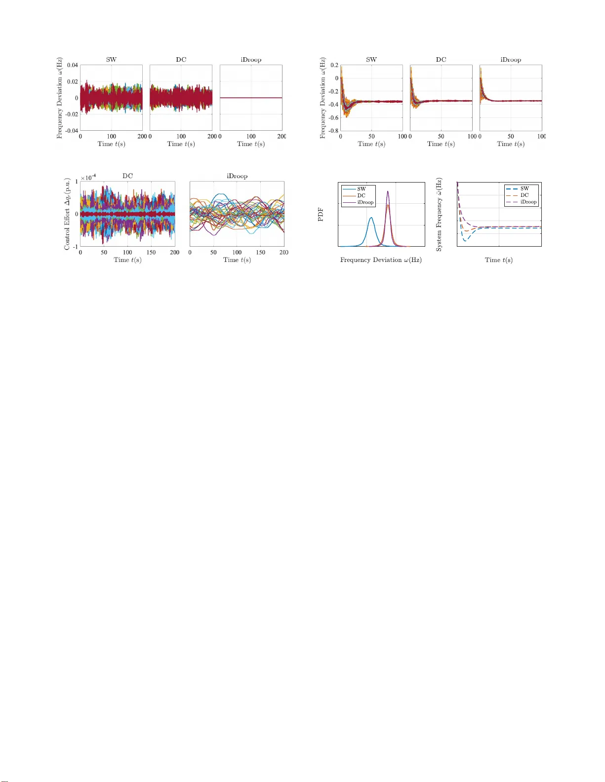
1 Dynamic Droop Control in Lo w-inertia Po wer Systems Y an Jiang, Richard Pates, and Enrique Mallada Abstract —A widely embraced approa ch to mitigate the dy- namic degradation in low-inertia power systems is to mimic generation response using grid-connected inv erters to restore the grid’s stiffness. In this paper , we see k to challenge this approach and adv ocate for a principled design based on a systematic a nalysis of the perf ormance trade-offs of inv erter- based frequency contro l. With this aim, we perf orm a qualitative and quantitative s tudy comparing the effect of con ventional control strategies –droop control (DC) and virtual inertia (VI)– on several performance metrics induced b y L 2 and L ∞ signal norms. By extendin g a recently proposed modal decomposition method, we capture th e effect of step a nd stochastic power disturbances, and frequency m easurement n oise, on the o vera ll transient and steady-state behavior of the system. Our analysis un veils several limitations of these solutions, such as the in- ability of DC to impr ov e dynamic frequency response with out increasing steady-state contro l effo rt, or the large frequency variance that VI introduces in the presence of mea surement noise. W e further propose a novel dynam-i-c Droop controller (iDroop) that ov ercomes th e limitations of DC and VI. More precisely , we show that iDro op can be tuned to achiev e high noise rejection, fast system-wide synchronization, or f requency ov ershoot (Nadir) elimination wit hout affectin g the steady-state control e ffo rt share , and propose a tuni ng recommendation that strikes a balance among these objectives. Extensive nu merical experimentation sh ows that the proposed tunin g is effectiv e even when our proportionality assumptions are not valid, and that the particular tun i ng used f or Na dir elimination strikes a g ood trade-off among various perfor mance metrics. I . I N T R O D U C T I O N The shift from conv entional synchro n ous genera tion to renewable converter -based sources has recen tly led to a n o- ticeable d egra d ation of the power system freq uency dynamics [3]. At the center of this problem is the reduc tion of the system-wide inertia th at accentu ates frequ ency ﬂuctu ations in resp onse to disturb ances [4], [5]. Besides increasing the risk of freq uency instabilities and blackouts [6], this dynam ic degradation also places limits on th e total amo unt of r enew able generation that can be sustained b y the grid [ 7]. Ireland , for instance, is alread y re so rting to wind curtailmen t wh e never wind becomes larger than 50 % of existing d emand in o rder to preserve the g rid stability [ 8]. A wid ely emb raced app roach to mitigate this problem is to mimic synch ronou s generation r esponse using grid- connected conv erters [9]. That is, to in troduce virtual inertia to restore the stiffness that the system used to enjoy [10]. Notable works within this line o f r esearch focus on leveraging comp utational methods [11]–[1 3] to efﬁciently allocate synthetic iner tial This material is supported by AR O through contract W911NF- 17-1-0092, US DoE EE RE award de-ee000 8006 , NSF through grants CNS 1544771, EPCN 1711188, AMPS 1736448, and CAREER 1752362, the Swedish Foundation for Strate gic Research, and the Swedish Re- search Council through the LCCC L innaeus Center . Y . Jiang and E. Mallad a are with the Johns Hopkins Univ ersity , Baltimore , MD 21218, USA. Emails: { yjia ng,mallada } @jhu.edu . Ri chard Pate s is with the Lund Univ ersity , Box 118, SE-221 00 Lund, Sweden. Email: richard.pates@ control.lth.se . A pre liminary version of part of the results in this paper has been presented in [1] and [2]. or droo p respon se, or analytica l m ethods that character ize the sensiti vity of different perfo rmance metrics to glo bal or spatial variations o f system par ameters [14]–[1 6]. Howe ver , to this day , it is unclear whe th er this particular choice of control is the most suitable for th e task. On the one h and, unlike synchro nous generato r s that leverage store d kinetic energy to modu late electric power in jection, conv erter-based controller s ne e d to activ ely change their power injection based on noisy measurem ents of frequency or po wer . On the other hand, con verter -based con trol can be sign iﬁcantly faster than conv entional gene rators. Th erefore , using converters to mimic generato r behavior does not ta ke ad vantage of their full potential. In this paper, we seek to ch allenge this appro ach of mimicking gen eration respo n se and adv ocate for a princ ip led control design perspecti ve. T o achie ve this goal, we build on recent efforts by the control community o n qu antifying po wer network dynamic perfor mance u sing L 2 and L ∞ norms [1 1], [17], and perfo rm a systema tic study ev aluating the effect of different con tr ol strategies, such as d roop control (DC) [18] and virtual inertia (VI) [19], on a set o f static and dynamic ﬁgures of merits that are practically r elev an t from the p ower e n gineerin g stand point. More precisely , under a mild –yet insightful– propor tio nality assumption, we co mpute closed form solutions an d sensi- ti vities of controller parameters on the steady-state control effort share, frequency Nadir, L 2 -synchro nization cost, and frequen cy variance of the respo nse of a power network to step and stochastic distur b ances. Ou r analysis unveils the inability of DC and VI to cop e with seemin gly oppo sing objectives, such as synchr onization cost reduc tion without incr e asing steady-state effort share (DC), or frequen cy Nadir reduc tio n without hig h frequ ency v ariance (VI). Th e refore, rather th a n clinging to the id e a of efﬁciently allocatin g syn thetic in e rtia or dro op, we advocate the sear ch of a better solu tion. T o this en d, w e prop ose novel dy nam-i-c D r oop (iDr oop) control –in spired by classical lead /lag com p ensation– which outperf orms cu rrent control strategies (VI and DC) in an overall sense. More p recisely: • U n like DC that sacriﬁces steady-state effort s hare to imp rove dynamic p erforma n ce, the adde d degrees of iDro op allow to deco uple steady-state effort from dynamic perfo rmance improvement. • U n like VI tha t ampliﬁes freq uency me a su rement noise, th e lead/lag pr operty of iDroo p makes it less sen siti ve to noise and power disturb ances, as mea su red by the H 2 norm [ 20] of the in put-ou tput system d e ﬁn ed from measuremen t no ise and power ﬂuctua tions to fre q uency d eviations. • iDr oop can further be tun ed to e ith er eliminate the frequency Nadir, b y comp ensating for the turb in e lag, or to eliminate synchro n ization cost; a feature shown to be unattainab le by virtual iner tia contro l. All of a bove prop erties are attained thr ough r igorou s analy- sis on explicit expre ssion s fo r p erforma nce metrics that are 2 achieved un der a mild yet in sightful prop ortionality ass ump- tion that generalizes prior work [1 ], [2]. W e further validate our analysis through extensi ve numerical simulations, per f ormed on a low-inertia system –the I celandic Grid– that does no t satisfy our param e ter assumptio n s. Our numerical results also show that iDr oop with the Nadir elim- inated tun ing designed b ased on the propor tional parame ter assumption works well even in environments with mixed step and stoch a stic disturbances. The rest of this p aper is organized as fo llows. Section I I describes the power n etwork model and deﬁnes perform ance metrics. Section III in troduce s our ass umption s and a sys- tem diag onalization that eases th e comp utations and de r iv es some g eneric results that p r ovide a f oundatio n for furth er perfor mance analysis. Section IV analyzes both steady-state and d ynamic perfo rmance of DC and VI, illustrates their limitations, and motiv ates the need fo r a new contr ol strategy . Section V describes th e prop osed iDroop and sh ows how it outperf orms DC and VI fr o m different p erspectives. Section VI validates ou r results thr o ugh detailed simulations. Section VII conclud e s the paper . I I . P R E L I M I N A R I E S A. P ower S ystem Mod el W e consider a con nected p ower network co mposed of n buses indexed by i ∈ V := { 1 , . . . , n } and transmission lines denoted b y u norde r ed pair s { i, j } ∈ E , where E is a set of 2 -element subsets of V . As illustrated b y th e blo c k diagram in Fig. 1, the system d ynamics are m odeled as a f eedback intercon nection of bus dy n amics and network dynamics. Th e in put sign als p in := ( p in ,i , i ∈ V ) ∈ R n and d p := ( d p ,i , i ∈ V ) ∈ R n represent power injection set point cha n ges an d power ﬂuctuations ar o und th e set po in t, respectively , an d n ω := ( n ω ,i , i ∈ V ) ∈ R n represents fre- quency m easurement no ise. T h e we ig hting f unctions ˆ W p ( s ) and ˆ W ω ( s ) can be used to ad just the size of these disturban ces in the usual way . The o utput signal ω := ( ω i , i ∈ V ) ∈ R n represents the bus freq uency de viation fro m its no minal value. W e now d iscuss the d y namic elements in more detail. 1) Bus Dyn a mics: The bus d ynamics that m aps the n et power bus imbalance u P = ( u P ,i , i ∈ V ) ∈ R n to th e vector o f frequ ency deviations ω can be describe d as a feedback loop that comprises a f orward-path ˆ G ( s ) and a feedback -path ˆ C ( s ) , where ˆ G ( s ) := diag ( ˆ g i ( s ) , i ∈ V ) and ˆ C ( s ) := diag ( ˆ c i ( s ) , i ∈ V ) are the transfer functio n matrices of gen erators and inverters, respec tively . a) Generator Dyna mics: T h e gen erator dy n amics are composed of the stan dard swing equations with a tur b ine, i.e. , m i ˙ ω i = − d i ω i + q r ,i + q t ,i + u P ,i , (1) where m i > 0 denotes the ag gregate generator in ertia, d i > 0 the agg regate gener ator dampin g, q r ,i the con trollable in put power produ ced by the grid-co nnected in verter , and q t ,i the change in the mech a n ical p ower outp ut o f the tu rbine. The turbine do es not react to the frequ ency deviation ω i until it exceeds a p reset thresho ld ω ǫ ≥ 0 , i.e., τ i ˙ q t ,i = ϕ ω ǫ ( ω i ) − q t ,i (2) ˆ C ( s ) = d iag (ˆ c i ( s ) , i ∈ V ) ˆ g 1 ( s ) ˆ g i ( s ) ˆ g n ( s ) Generator Dynamics ˆ G ( s ) = diag (ˆ g i ( s ) , i ∈ V ) u P L B s Network Dynamics p e p in − + Inverter Dynamics + + n ω ω ˆ c 1 ( s ) ˆ c i ( s ) ˆ c n ( s ) q r Bus Dynamics ω m d p ˆ W p ( s ) ˆ W ω ( s ) Fig. 1 : Block d iagram of p ower n etwork. with ϕ ω ǫ ( ω i ) :=      − r − 1 t ,i ( ω i + ω ǫ ) ω i ≤ − ω ǫ 0 − ω ǫ < ω i < ω ǫ − r − 1 t ,i ( ω i − ω ǫ ) ω i ≥ ω ǫ , where τ i > 0 represents the turbine time constant and r t ,i > 0 the turbin e droo p coefﬁcient. T w o special cases o f ou r interest are : Generator Dyna mics 1 (Sta ndard swing dyna mics). When | ω i ( t ) | < ω ǫ , th e turbine s ar e not trigger ed a nd the generator dynamics can b e d e scribe d by the tr ansfer function ˆ g i ( s ) = 1 m i s + d i (3) which is exactly the stan dar d swing dyn amics. Generator Dynamics 2 (Second-order turbine dy namics). When ω ǫ = 0 , the turb in es ar e constan tly trigger ed and the generator dynamics ca n be described by the transfer func tion ˆ g i ( s ) = τ i s + 1 m i τ i s 2 + ( m i + d i τ i ) s + d i + r − 1 t ,i . (4) b) In v e rter Dyn amics: Since power electronics are sig- niﬁcantly faster tha n the electro -mechanic a l dynamics of g e n- erators, we assume th at each inverter measures the local g rid frequen cy d eviation ω i and instantaneou sly updates th e outp ut power q r ,i . Different control laws ca n be used to ma p ω i to q r ,i . W e represent such laws u sing a transfer functio n ˆ c i ( s ) . The two m ost commo n ones are: In verter Dynamics 1 (Droop Co ntrol). Th is contr ol law can pr ovide a dditiona l dr o o p capa bilities and is given b y ˆ c i ( s ) = − r − 1 r ,i , (5) wher e r r ,i > 0 is the dr o op coefﬁcient. 3 In verter Dynamics 2 (Virtual Inertia). Be sid e s pr oviding addition al dr oop capa bilities, th is contr ol law can compensate the lo ss of inertia and is g iv e n by ˆ c i ( s ) = −  m v ,i s + r − 1 r ,i  , (6) wher e m v ,i > 0 is the virtual inertia co nstant. 2) Network Dyna mics: The network power ﬂu c tu ations p e := ( p e ,i , i ∈ V ) ∈ R n are g i ven by a linearized model of the po wer ﬂow e q uations [21]: ˆ p e ( s ) = L B s ˆ ω ( s ) , (7) where ˆ p e ( s ) and ˆ ω ( s ) de note the Laplac e transform s of p e and ω , respectively . 1 The ma tr ix L B is an u n directed weighted Laplacian matrix of th e ne twork with elements L B ,ij = ∂ θ j n X j =1 | V i || V j | b ij sin( θ i − θ j )    θ = θ 0 . Here, θ := ( θ i , i ∈ V ) ∈ R n denotes the ang le d eviation from its nominal, θ 0 := ( θ 0 ,i , i ∈ V ) ∈ R n are the equilibrium angles, | V i | is the (constant) voltage magnitud e at bus i , and b ij is th e line { i, j } suscep tance. 3) Closed-loop Dynamics: W e will in vestigate the closed- loop respo nses of th e system in Fig . 1 from the power injection set po int changes p in , the power ﬂuc tu ations aro und the set point d p , and frequen cy measure m ent n oise n ω to frequ ency deviations ω , which can be descr ibed compactly by the transfer function ma tr ix ˆ T ( s ) := h ˆ T ω p ( s ) ˆ T ω dn ( s ) :=  ˆ T ω d ( s ) ˆ T ω n ( s )  i . (8) Remark 1 (Model Assumptions). The line arized n etwork model ( 8) implicitly makes the follo wing assumptions which ar e standar d and well-justiﬁed for fr equency contr ol on trans- mission ne tworks [22]: • Bus vo ltage magnitudes | V i | ’ s ar e co nstant; we are not modeling th e dyna mics of exciter s used for voltage contr o l; these ar e assumed to operate at a much faster time-scale. • Lines { i, j } ar e lossless. • Reactive power ﬂows do n ot affect bus voltage phase ang les and fr equencies. • W ithout loss of generality , the equilibrium a ngle dif fer en ce ( θ 0 ,i − θ 0 ,j ) a c c r oss ea ch line is less th an π / 2 . F or a ﬁrst principle d erivation of the model w e r efer to [23, Section VII]. F or application s of similar mod els for fr equency contr o l within th e contr ol literatur e, see, e.g., [24]–[26]. Remark 2 (Intern al Stability of (8) ). Thr ougho ut this pap er we consider fee dback inter connectio ns of positive real a nd strictly p ositive real subsystems. Internal stability follows fr om cla ssical r esults [27]. Since the focus of this p aper is on performan ce, we do not d iscu ss internal stability her e in detail. W e refer to th e r ea der to [28], fo r a thor ough tr ea tment of similar feedback interconnections. F r om now on a standing assumption –that can be veriﬁed– is that feedback inter connection described in F ig. 1 is internally stable. 1 W e use hat to distingui sh the Laplace transform from its time domain counter part. B. P erformance Metr ics Having con sidered the model of the p ower network, we are now read y to introduce perform a nce metrics used in this paper to comp are different inverter con trol laws. 1) Steady-state Effort S har e: T his m e tr ic m easures the fraction of the power imbalan ce addr essed by inv erters, which is calculated as the ab solute value of the ratio between the in- verter steady- state input power and the total power imbalance , i.e., ES :=     P n i =1 ˆ c i (0) ω ss ,i P n i =1 p in ,i (0 + )     , (9) when the system ˆ T ω p undergoes a step change in power excitation. Here, ˆ c i (0) is the dc gain of th e inverter and ω ss ,i is the steady-state frequen cy deviation. 2) P ower Fluctua tio ns and Measur ement Noise: This met- ric measures how the relativ e intensity of power ﬂuctuation s and measureme n t noise affect the frequen cy deviations, as quantiﬁed by the H 2 norm of the transfer fu nction ˆ T ω dn : k ˆ T ω dn k 2 H 2 (10) :=    1 2 π Z ∞ −∞ tr  ˆ T ω dn ( j ω ) ∗ ˆ T ω dn ( j ω )  d ω if ˆ T ω dn is stab le , ∞ otherwise. 2 The quantity k ˆ T ω dn k H 2 has sev eral stan d ard interpretatio n s in terms o f the inp ut-outp ut behavior of the system ˆ T ω dn [20]. In pa r ticular, in the stochastic setting, w h en the disturban ce signals d p ,i and n ω ,i are indep e n dent, zero mean , u n it variance, white noise, th en lim t →∞ E  ω ( t ) T ω ( t )  = k ˆ T ω dn k 2 H 2 . This means that th e sum of the stead y-state variances in the output of ˆ T ω dn in response to these disturban ce equals the squared H 2 norm of ˆ T ω dn . Thus the H 2 norm giv es a precise m easure of h ow the in ten sity of power ﬂuctuations and measu r ement noise affects the system ’ s fre quency d eviations. 3) Synchr onization Cost: This metric m e asures the size of individual bus deviations fr om the sy n chron o us r esponse wh en the system ˆ T ω p is subject to a step c hange in power excitation giv en by p in = u 0 1 t ≥ 0 ∈ R n , wh ere u 0 ∈ R n is a given vector dir ection an d 1 t ≥ 0 is the unit-step f unction [17]. This is quantiﬁed by the squared L 2 norm of the vector of d eviations ˜ ω := ω − ¯ ω 1 n ∈ R n , i.e., k ˜ ω k 2 2 := n X i =1 Z ∞ 0 ˜ ω i ( t ) 2 d t . (11) Here, ¯ ω := ( P n i =1 m i ω i ) / ( P n i =1 m i ) is the system frequency that corr esponds to th e inertia-we ig hted average of bus fre- quency d eviations and 1 n ∈ R n is the vector of all o nes. 4) Nadir: This metric measures the m inimum post- contingen cy frequ ency of a power system, which can be quantiﬁed by the L ∞ norm o f the system frequency ¯ ω , i. e . , k ¯ ω k ∞ := max t ≥ 0 | ¯ ω ( t ) | , (12) when th e system ˆ T ω p has as inpu t a step chan ge in power excitation [1 7], i. e., p in = u 0 1 t ≥ 0 ∈ R n . This quantity matters in that deeper Nadir incr eases the risk of un der-frequency lo ad shedding an d cascading outrages. 2 j represe nts the imaginary unit which satisﬁes j 2 = − 1 and ω represent s the frequenc y var iable . 4 I I I . R E S U LT S In this section we show that under a simplify ing assumption, it is po ssible to co mpute all of th e p erform a n ce metrics introdu c ed in Section II-B analytica lly as fu nctions of the system par a meters, which pave us a way to fo rmally compar e the conv entional contro l laws DC and VI in Section IV as well as sugg est an improved con trol law iDroop in Section V. W e remark that th e assumptions are o nly used in the analysis, but as we show in Section VI th e insights and advantages of the propo sed solu tio n are still there wh en these assump tions do not ho ld . A. Diagonalization In orde r to ma ke the an alysis tractable, we require the closed-loo p transfer fun ctions to be diagonalizable. This is ensured b y the f o llowing a ssum ption, which is a g eneralization of [15], [17]. Assumption 1 (Proportionalit y ). Ther e exists a pr oportion- ality ma trix F := diag ( f i , i ∈ V ) ∈ R n × n ≥ 0 such that ˆ G ( s ) = ˆ g o ( s ) F − 1 and ˆ C ( s ) = ˆ c o ( s ) F wher e ˆ g o ( s ) and ˆ c o ( s ) ar e called the r e p r e sentative generator and th e r epr esentative inverter , r espectively . Remark 3 (P roportionality parameters). The parameters f i ’ s r epr esent the individ ual ma chine rating. This d eﬁnition is rather a rbitrary for o u r ana ly sis, pr ovided that A ssump tion 1 is satisﬁed. Other alternatives cou ld includ e f i = m i or f i = m i /m wher e m is, for example, either the averag e or maximu m gen e rator inertia. The practical rele vance of Assumption 1 is justiﬁed, for example, by the e m p irical v a lues r ep orted in [29], which sho w that at least in r e g ar ds of or der of magnitude, Assump tion 1 is a r ea so nable ﬁrst-cut appr oximation to heter ogeneity . Under Assumption 1, the rep resentative gen e r ator o f (3) and (4) are gi ven by ˆ g o ( s ) = 1 ms + d (13) and ˆ g o ( s ) = τ s + 1 mτ s 2 + ( m + dτ ) s + d + r − 1 t , 3 (14) respectively , with m i = f i m , d i = f i d , r t ,i = r t /f i , an d τ i = τ . Similarly , the r epresentative inverters of DC (5) a n d VI (6) are given by ˆ c o ( s ) = − r − 1 r (15) and ˆ c o ( s ) = −  m v s + r − 1 r  , (16) with m v ,i = f i m v and r r ,i = r r /f i . Using Assumptio n 1, we can d eriv e a diag onalized version of (8). First, we rewrite ˆ G ( s ) = F − 1 2 [ ˆ g o ( s ) I n ] F − 1 2 and ˆ C ( s ) = F 1 2 [ˆ c o ( s ) I n ] F 1 2 3 W e use vari ables without subscript i to denote paramet ers of represe n- tati ve generato r and in vert er . as s hown in Fig. 2(a), an d af ter a loop transformatio n obtain Fig. 2(b ). Then, we deﬁn e the scaled Laplacian matrix L F := F − 1 2 L B F − 1 2 (17) by gr o uping th e terms in the u pper block o f Fig. 2(b) . More- over , s ince L F ∈ R n × n is symmetric po siti ve semideﬁnite, it is rea l ortho gonally diagona liza b le with non-n egative eig en val- ues [30]. Thus, there e xists an orthogonal m atrix V ∈ R n × n with V T V = V V T = I n , such that L F = V Λ V T , (18) where Λ := dia g ( λ k , k ∈ { 1 , . . . , n } ) ∈ R n × n ≥ 0 with λ k being the k th eigenv alue of L F ordered non-decr easingly (0 = λ 1 < λ 2 ≤ . . . ≤ λ n ) 4 and V :=  ( P n i =1 f i ) − 1 2 F 1 2 1 n V ⊥  with V ⊥ :=  v 2 . . . v n  composed by the eigenvector v k associated with λ k . 5 Now , ap plying (17) and (18) to Fig. 2 (b) and rearran ging blo cks of V and V T results in Fig. 2(c). Finally , movin g th e block of ˆ c o ( s ) I n ahead o f the summing junction and combinin g the two parallel path s pro d uces Fig. 3, where the boxed part is fully diagona lize d. Now , by deﬁning the clo sed-loop with a forward-p ath ˆ g o ( s ) I n and a feedback-pa th (Λ /s − ˆ c o ( s ) I n ) a s ˆ H p ( s ) = diag  ˆ h p ,k ( s ) , k ∈ { 1 , . . . , n }  where ˆ h p ,k ( s ) = ˆ g o ( s ) 1 + ˆ g o ( s ) ( λ k /s − ˆ c o ( s )) , (19) and ˆ H ω ( s ) = ˆ c o ( s ) ˆ H p ( s ) , i.e., ˆ H ω ( s ) = diag  ˆ h ω ,k ( s ) , k ∈ { 1 , . . . , n }  where ˆ h ω ,k ( s ) = ˆ c o ( s ) ˆ h p ,k ( s ) , (20) the closed-loop transfer functions from p in , d p , and n ω to ω become ˆ T ω p ( s ) = F − 1 2 V ˆ H p ( s ) V T F − 1 2 , (21a) ˆ T ω d ( s ) = F − 1 2 V ˆ H p ( s ) V T F − 1 2 ˆ W p ( s ) , (21b) ˆ T ω n ( s ) = F − 1 2 V ˆ H ω ( s ) V T F 1 2 ˆ W ω ( s ) , (21c) respectively . Note that dependin g on the speciﬁc generator a nd in verter dynamics inv o lved, we may add subscrip ts in the nam e of a transfer func tio n without making a fu rther declaratio n in the rest of this paper . For example, we may add ’T’ if the turbine is tr iggered and ’DC’ if the in verter operates in DC mod e as in ˆ h p ,k, T , DC ( s ) . B. Generic R esults for P erformance Metr ics W e now derive so m e important building block s requ ired for the performan c e analysis of the system ˆ T d escribed in (21). As described in Section II-B, th e sensitivity to power ﬂuctuations and measurement no ise can be evaluated thr ough the H 2 norm of the system ˆ T ω dn , while the steady-state effort share, synchr onization c o st, and Nadir can all be characterized 4 Recal l tha t we assume the po wer netw ork is connected, which means that L F has a single eigen val ue at the origin. 5 W e use k and l to index dynamic modes but i and j to index bus numbers. 5 u P L B s p e p in − + + + ω q r F − 1 2 ˆ g o ( s ) I n F − 1 2 F 1 2 ˆ c o ( s ) I n F 1 2 ω m d p ˆ W p ( s ) n ω ˆ W ω ( s ) (a) L B s p in + + ω ˆ g o ( s ) I n F − 1 2 F − 1 2 F − 1 2 F 1 2 ˆ c o ( s ) I n F − 1 2 − + d p ˆ W p ( s ) n ω ˆ W ω ( s ) (b) p in + + ω ˆ g o ( s ) I n ˆ c o ( s ) I n − Λ s F − 1 2 F 1 2 V T V V T F − 1 2 p in + d p ˆ W p ( s ) n ω ˆ W ω ( s ) (c) Fig. 2 : Equ i valent block d iagrams of power network un der prop o rtionality assumption. + ω ˆ g o ( s ) I n − F − 1 2 F 1 2 ˆ c o ( s ) I n Λ s − ˆ c o ( s ) I n + ˆ H p ( s ) V T V F − 1 2 V T ˆ H ω ( s ) + d p ˆ W p ( s ) p in ˆ W ω ( s ) n ω Fig. 3 : Diago nalized b lock diag ram of power network. by a step response o f the system ˆ T ω p . T here ar e two scenar io s that ar e of ou r interest. Assumption 2 (Proportional weighting scenario). • The noise weighting functions ar e given by ˆ W p ( s ) = κ p F 1 2 and ˆ W ω ( s ) = κ ω F − 1 2 , wher e κ p > 0 a nd κ ω > 0 a r e weighting constants. • | ω i ( t ) | < ω ǫ , ∀ i ∈ V and t ≥ 0 such that turbines will not be trigger ed. Assumption 3 (Step inp ut scenario). • Ther e is a step change as deﬁned in Section II - B on the power injection set point, i.e., p in = u 0 1 t ≥ 0 , d p = 0 n , an d n ω = 0 n with 0 n ∈ R n being the vector o f all zer os. • ω ǫ = 0 su ch th at turb ines ar e constantly tr igger ed. Remark 4 (W eig hting assumption). As a natural cou nter- part of Assumption 1, we look at the ca se when th e power ﬂuctuatio ns a nd measur ement noise ar e weighted d ir ec tly and in versely p r oportiona l to the squa r e r oot of the bus ratings, r esp ectively . In the case o f ˆ W p ( s ) , this is equiv a lent to assuming that deman d ﬂuctu ation variances ar e pr opo rtional to the bus ratings, which is in agr eement with the central limit theor em. F or ˆ W ω ( s ) , this is equivalent to assuming th e fr eq uency measurement n oise variances a r e in ve rsely pr opor- tional to the bus ratings, which is in line with the in ve rse r ela tionship between jitter va riance and p ower consump tion for an oscillator in phase-locked-loop [31]. 1) Steady-state Effort S har e: As indicated by (9), the key of computin g the steady-state effort share lies in computing the steady-state frequen cy de viation ω ss of the system ˆ T ω p . When the system synchronizes, the steady - state freque n cy deviation is given by ω ss = ω syn 1 n and ω syn is ca lled the sync hrono u s frequen cy . In the ab sence o f a seconda ry contr ol layer, e.g., automatic generation co ntrol [32], the system ca n sy nchron ize with a n ontrivial fr equency deviation, i.e. , ω syn 6 = 0 . The following lemma p rovides a gener al expression for ω syn in our sett ing. Lemma 1 (Synchronous frequency). Let Assumption 3 ho ld. If q r ,i is determined by a contr ol la w ˆ c i ( s ) , then the o utput ω of the system ˆ T ω p synchr onizes to the steady-state fr equency deviation ω ss = ω syn 1 n with ω syn = P n i =1 u 0 ,i P n i =1  d i + r − 1 t ,i − ˆ c i (0)  . (22) Pr oo f. Combining (1) and (7) thro ugh the relatio nship u P = p in − p e , we get th e ( p artial) state-space representa tio n of the system ˆ T ω p as ˙ θ = ω , (23a) M ˙ ω = − D ω − L B θ + q r + q t + p in , (23b) where M := diag ( m i , i ∈ V ) ∈ R n × n ≥ 0 , D := diag ( d i , i ∈ V ) ∈ R n × n ≥ 0 , q r := ( q r ,i , i ∈ V ) ∈ R n , and q t := ( q t ,i , i ∈ V ) ∈ R n . In steady-state, (23) yields L B ω ss t = − D ω ss − L B θ ss 0 + q r , ss + q t , ss + u 0 , (24) where ( θ ss 0 + ω ss t, ω ss , q r , ss , q t , ss ) denotes the steady-state so- lution of (2 3). Equation (24) ind icates that L B ω ss t is con stant and thus L B ω ss = 0 n . It fo llows that ω ss = ω syn 1 n . The r efore, (24) beco mes 0 n = − D ω syn 1 n − L B θ ss 0 + q r , ss + q t , ss + u 0 , (25) where q r , ss = ( ˆ c i (0) ω syn , i ∈ V ) ∈ R n and q t , ss =  − r − 1 t ,i ω syn , i ∈ V  ∈ R n when ω ǫ = 0 by (2). Pre-mu ltiplying (25) by 1 T n and using the prop erty that 1 T n L B = 0 T n , we get the desired result in (22). Now , the theorem below provides an explicit expression for the steady-state ef f o rt share. Theorem 1 (Steady- state effort sha re). Let Assumption 3 hold. If q r ,i is determined by a c o ntr ol law ˆ c i ( s ) , then the 6 steady-state effort share of the sys tem ˆ T ω p is g iven by ES =      P n i =1 ˆ c i (0) P n i =1  d i + r − 1 t ,i − ˆ c i (0)       . (26) Pr oo f. It follows directly from Lemma 1 that ω ss ,i = ω syn and P n i =1 u 0 ,i = ω syn P n i =1  d i + r − 1 t ,i − ˆ c i (0)  . Plugg ing these two equ ations to the deﬁnition of ES in (9) y ields th e desired result. 2) P ower Flu ctuations a nd Measur ement Noise: W e seek to characte r ize the effect of power ﬂuc tu ations an d frequency measuremen t noise o n the freque n cy variance, i.e., the H 2 norm of the system ˆ T ω dn . W e ﬁrst show that the squ ared H 2 norm o f ˆ T ω dn is a weighted sum of the squared H 2 norm of each ˆ h p ,k and ˆ h ω ,k in th e diagonalized sy stem (21). Theorem 2 (Frequency variance) . De ﬁne Γ := V T F − 1 V . If Assumptions 1 and 2 h old, then k ˆ T ω dn k 2 H 2 = n X k =1 Γ kk  κ 2 p k ˆ h p ,k k 2 H 2 + κ 2 ω k ˆ h ω ,k k 2 H 2  . Pr oo f. It follows fro m (8) and (10 ) that k ˆ T ω dn k 2 H 2 = 1 2 π Z ∞ −∞ tr  ˆ T ω d ( j ω ) ∗ ˆ T ω d ( j ω )  d ω + 1 2 π Z ∞ −∞ tr  ˆ T ω n ( j ω ) ∗ ˆ T ω n ( j ω )  d ω =: k ˆ T ω d k 2 H 2 + k ˆ T ω n k 2 H 2 . W e n ow compu te k ˆ T ω d k 2 H 2 . Using (21b) and the fact that ˆ W p ( s ) = κ p F 1 2 by Assum p tion 2, we get ˆ T ω d ( s ) = κ p F − 1 2 V ˆ H p ( s ) V T . Th erefore, ˆ T ω d ( j ω ) ∗ ˆ T ω d ( j ω ) = κ 2 p V ˆ H p ( j ω ) ∗ V T F − 1 V ˆ H p ( j ω ) V T . Using the c yclic pro perty o f th e trace, this implies that tr  ˆ T ω d ( j ω ) ∗ ˆ T ω d ( j ω )  = κ 2 p tr  ˆ H p ( j ω ) ∗ Γ ˆ H p ( j ω )  , where Γ := V T F − 1 V . Therefo re, it follows that k ˆ T ω d k 2 H 2 = 1 2 π Z ∞ −∞ κ 2 p tr  ˆ H p ( j ω ) ∗ Γ ˆ H p ( j ω )  d ω = n X k =1 κ 2 p Γ kk 2 π Z ∞ −∞    ˆ h p ,k ( j ω )    2 d ω = κ 2 p n X k =1 Γ kk k ˆ h p ,k k 2 H 2 . The result f ollows fro m a similar argu ment on k ˆ T ω n k 2 H 2 . Theorem 2 allo ws us to compute the H 2 norm of ˆ T ω dn by means of comp u ting the nor ms of a set of simple scalar tr a n sfer function s. However , f or different co n trollers, the transfer func- tions ˆ h p ,k and ˆ h ω ,k will change. Since in all the cases these transfer func tio ns are of fourth-o rder or lower , the following lemma will suf ﬁce for the p u rpose of o ur comp arison. Lemma 2 ( H 2 norm of a fourth-order transfer function). Let ˆ h ( s ) = b 3 s 3 + b 2 s 2 + b 1 s + b 0 s 4 + a 3 s 3 + a 2 s 2 + a 1 s + a 0 + b 4 be a stable transfer function. If b 4 = 0 , then k ˆ h k 2 H 2 = ζ 0 b 2 0 + ζ 1 b 2 1 + ζ 2 b 2 2 + ζ 3 b 2 3 + ζ 4 2 a 0 ( a 1 a 2 a 3 − a 2 1 − a 0 a 2 3 ) , (27) wher e ζ 0 := a 2 a 3 − a 1 , ζ 1 := a 0 a 3 , ζ 2 := a 0 a 1 , (2 8 ) ζ 3 := a 0 a 1 a 2 − a 2 0 a 3 , ζ 4 := − 2 a 0 ( a 1 b 1 b 3 + a 3 b 0 b 2 ) . Otherwise, k ˆ h k 2 H 2 = ∞ . Pr oo f. First recall that gi ven an y state-space realization of ˆ h ( s ) , the H 2 norm can be calc u lated by solving a par ticular L yapun ov equ a tio n. Mo re speciﬁcally , s uppose Σ ˆ h ( s ) =  A B C D  , and let X d enote the solution to the L yapunov eq uation AX + X A T = − B B T . (29) If ˆ h ( s ) is stable, then k ˆ h k 2 H 2 = ( ∞ if D 6 = 0 , C X C T otherwise . (30) Consider the observ able canonical for m of ˆ h ( s ) given by Σ ˆ h ( s ) =      0 0 0 − a 0 b 0 1 0 0 − a 1 b 1 0 1 0 − a 2 b 2 0 0 1 − a 3 b 3 0 0 0 1 b 4      . ( 31) Since D = b 4 , it is trivial to see fr om (30) that if b 4 6 = 0 then k ˆ h k 2 H 2 = ∞ . Hence, in th e r est of the proof, we assume b 4 = 0 . W e will now solve the L yap unov eq uation analy tically for the realization (31). X must be symm etric an d thus can be param eterized as X =  x ij  ∈ R 4 × 4 , with x ij = x j i . (32) Since it is easy to see th a t C X C T = x 44 , the pr oblem becomes solving fo r x 44 . Substituting (3 1) and (32) into (29 ) yields the follo wing equation s 2 a 0 x 14 = b 2 0 , (33a) x 12 − a 2 x 14 − a 0 x 34 = − b 0 b 2 , (33b) 2( x 12 − a 1 x 24 ) = − b 2 1 , (33c) x 23 − a 3 x 24 + x 14 − a 1 x 44 = − b 1 b 3 , (33d) 2( x 23 − a 2 x 34 ) = − b 2 2 , (33e) 2( x 34 − a 3 x 44 ) = − b 2 3 . (33f) Throu g h stand ard algebra, we can solve for x 44 as x 44 = ζ 0 b 2 0 + ζ 1 b 2 1 + ζ 2 b 2 2 + ζ 3 b 2 3 + ζ 4 2 a 0 ( a 1 a 2 a 3 − a 2 1 − a 0 a 2 3 ) with ζ 0 , ζ 1 , ζ 2 , ζ 3 , an d ζ 4 deﬁned by (28), wh ic h conclu des the proof; the denomina tor is guar anteed to be no nzero by the Routh-Hur witz cr iterion. Remark 5 ( H 2 norm of a t ransfer function lower than fourth-order). Alth o ugh Lemma 2 is stated for a fo urth-order transfer fun ction, it can also be used to ﬁn d the H 2 norm o f 7 thir d-, second -, an d ﬁrst-or der transfer functions by consid- ering appr opriate limits. F o r example, setting a 0 = b 0 = ǫ and considering the limit ǫ → 0 , (27) gives the H 2 norm of a generic th ir d -or der transfer functio n. This p r ocess shows tha t given a s table tr a nsfer fun ction ˆ h ( s ) , if b 4 = 0 a nd: • (thir d - or der transfer functio n) a 0 = b 0 = 0 , then k ˆ h k 2 H 2 = a 3 b 2 1 + a 1 b 2 2 + a 1 a 2 b 2 3 − 2 a 1 b 1 b 3 2 a 1 ( a 2 a 3 − a 1 ) ; • (second-order transfer function) a 0 = b 0 = a 1 = b 1 = 0 , then k ˆ h k 2 H 2 = b 2 2 + a 2 b 2 3 2 a 2 a 3 ; • (ﬁrst-or der transfer fu nction) a 0 = b 0 = a 1 = b 1 = a 2 = b 2 = 0 , then k ˆ h k 2 H 2 = b 2 3 2 a 3 ; otherwise k ˆ h k 2 H 2 = ∞ . Remark 6 ( W ell-deﬁnedness by the stability). Note that the stability o f ˆ h ( s ) guarantees that th e denomin ators in all the above H 2 norm expr essions a r e nonzer o by the Rou th-Hurwitz stability criterion . 3) Synchr onization Cost: The computation of the sync h ro- nization cost deﬁn e d in (11) for the sy stem ˆ T ω p in the absen ce of inverter control can be fou nd in [15]. T aking this into account, we can get co rrespon d ing results f o r the system with any contro l law r eadily . Lemma 3 (Synchronization cost). Let Assumptions 1 an d 3 hold. Deﬁn e ˜ u 0 := V T ⊥ F − 1 2 u 0 and ˜ Γ := V T ⊥ F − 1 V ⊥ . Then the synchr onizatio n cost of th e system ˆ T ω p is g iven by k ˜ ω k 2 2 = ˜ u T 0  ˜ Γ ◦ ˜ H  ˜ u 0 , wher e ◦ denotes the Hadamar d pr od u ct and ˜ H ∈ R ( n − 1) × ( n − 1) is the matrix with entries ˜ H kl := Z ∞ 0 h u ,k ( t ) h u ,l ( t ) d t , ∀ k , l ∈ { 1 , . . . , n − 1 } with ˆ h u ,k ( s ) := ˆ h p ,k +1 , T ( s ) /s and ˆ h p ,k, T ( s ) being a sp eciﬁed case of the transfer fun ction ˆ h p ,k ( s ) deﬁ ned in ( 19) , i.e., when the tu rbine is trigger ed. Pr oo f. This is a direct extension of [15, Proposition 2]. Lemma 3 shows that the compu tation of th e synch ronization cost requires knowing the inner produ cts ˜ H kl . Howe ver, the general expression s of these in ner pr oducts for an arb itrary combinatio n of k and l are already too tedious to be useful in our analy sis. Th erefore, we will inv estigate instead bo unds on th e sync h ronization cost in terms of the inner produ cts ˜ H kl when k = l ; which are exactly the H 2 norms o f tran sfer function s ˆ h u ,k ( s ) . Lemma 4 (Bounds for Hadamard product). Let P ∈ R n × n be a symmetric ma trix with minimum and ma ximum eigen- values given by λ min ( P ) and λ max ( P ) , res pectively . Then ∀ x, y ∈ R n , λ min ( P ) n X k =1 x 2 k y 2 k ≤ x T  P ◦  y y T  x ≤ λ max ( P ) n X k =1 x 2 k y 2 k . Pr oo f. First no te that x T  P ◦  y y T  x = tr  P T ( x ◦ y ) ( x ◦ y ) T  = ( x ◦ y ) T P T ( x ◦ y ) . Let w := x ◦ y . Since P is symmetric, by Ray leigh [30] λ min ( P ) w T w ≤ x T  P ◦  y y T  x ≤ λ max ( P ) w T w. Observing that w T w = P n k =1 x 2 k y 2 k completes the proof. Lemma 4 imp lies the following bounds on the synchroniza - tion cost. Theorem 3 (Bounds on synchr onization cost). Let Assump- tions 1 and 3 hold . Then th e syn chr onization cost of the system ˆ T ω p is b ounde d by k ˜ ω k 2 2 ≤ k ˜ ω k 2 2 ≤ k ˜ ω k 2 2 , where k ˜ ω k 2 2 := P n − 1 k =1 ˜ u 2 0 ,k k ˆ h u ,k k 2 H 2 max i ∈V ( f i ) and k ˜ ω k 2 2 := P n − 1 k =1 ˜ u 2 0 ,k k ˆ h u ,k k 2 H 2 min i ∈V ( f i ) . Pr oo f. By Lemma 3, k ˜ ω k 2 2 = Z ∞ 0 ˜ u T 0  ˜ Γ ◦  h u ( t ) h u ( t ) T   ˜ u 0 d t ≥ Z ∞ 0 λ min ( ˜ Γ) n − 1 X k =1 ˜ u 2 0 ,k h u ,k ( t ) 2 d t = λ min ( ˜ Γ) n − 1 X k =1 ˜ u 2 0 ,k k ˆ h u ,k k 2 H 2 ≥ λ min ( F − 1 ) n − 1 X k =1 ˜ u 2 0 ,k k ˆ h u ,k k 2 H 2 = P n − 1 k =1 ˜ u 2 0 ,k k ˆ h u ,k k 2 H 2 max i ∈V ( f i ) , which conc lu des the pr oof of the lower b ound. The ﬁrst inequality follows fr o m Lemma 4 by setting P = ˜ Γ , x = ˜ u 0 , and y = h u ( t ) := ( h u ,k ( t ) , k ∈ { 1 , . . . , n − 1 } ) ∈ R n − 1 . The secon d inequality follows f rom the in terlacing theor em [30, Theorem 4.3.1 7]. The upper bo und can be proved simi- larly . Remark 7 (Sy nchronization cost in homogeneous case). In the system with homogeneous parameters, i.e., F = f I n for some f > 0 , the identical lower and u pper bo u nds on the synchr onizatio n cost imply that k ˜ ω k 2 2 = f − 1 n − 1 X k =1 ˜ u 2 0 ,k k ˆ h u ,k k 2 H 2 . 4) Nadir: A deep Nadir poses a thr eat to the reliab le operation of a power system. Hence on e of th e goals of inv erter control laws is th e r e duction of Nad ir . W e seek to ev aluate the ability of different co n trol laws to eliminate Nadir . T o this end, w e provide a necessary and sufﬁcient condition fo r Nadir elimination in a second-o rder system with a zero. Theorem 4 (Nadir elimination for a second-order system). Assume K > 0 , z > 0 , ξ ≥ 0 , ω n > 0 . The step r espo n se of a second -or der system with transfer function given by ˆ h ( s ) = K ( s + z ) s 2 + 2 ξ ω n s + ω 2 n 8 has no N adir if and only if 1 ≤ ξ ≤ z /ω n or ( ξ > z / ω n ξ ≥ ( z / ω n + ω n /z ) / 2 , (34) wher e the con ditions in b races jo intly imply ξ > 1 . Pr oo f. Basically , Nadir mu st occ ur at some non-n egative ﬁnite time instant t nadir , such that ˙ p u ( t nadir ) = 0 and p u ( t nadir ) is a maximum , wher e p u ( t ) denotes the unit-step response of ˆ h ( s ) , i.e., ˆ p u ( s ) := ˆ h ( s ) /s . W e consider three cases based on the value o f damp ing ratio ξ separately: 1) Under damped case ( 0 ≤ ξ < 1 ): The output is ˆ p u ( s ) = K z ω 2 n  1 s − s + ξ ω n ( s + ξ ω n ) 2 + ω 2 d − ξ ω n − ω 2 n z − 1 ( s + ξ ω n ) 2 + ω 2 d  with ω d := ω n p 1 − ξ 2 , which gives the time dom ain response p u ( t ) = K z ω 2 n  1 − e − ξω n t η 0 sin ( ω d t + φ )  , where η 0 = s 1 +  ξ ω n − ω 2 n z − 1  2 ω 2 d and tan φ = ω d ξ ω n − ω 2 n z − 1 . Clearly , the above re sp onse must hav e oscillations. There - fore, for the case 0 ≤ ξ < 1 , Nadir a lways exists. 2) Critically damped case ( ξ = 1 ) : The ou tput is ˆ p u ( s ) = K z ω 2 n " 1 s − 1 s + ω n − ω n − ω 2 n z − 1 ( s + ω n ) 2 # , which gives th e time d omain respon se p u ( t ) = K z ω 2 n  1 − e − ω n t  1 +  ω n − ω 2 n z − 1  t  . Thus, ˙ p u ( t ) = K z e − ω n t  1 − ω n z − 1  t + z − 1  . Letting ˙ p u ( t ) = 0 yields ω n e − ω n t  1 +  ω n − ω 2 n z − 1  t  = e − ω n t  ω n − ω 2 n z − 1  , which has a non-negative ﬁnite solution t nadir = z − 1 ω n z − 1 − 1 whenever ω n z − 1 > 1 . F or any ǫ > 0 , it holds that ˙ p u ( t nadir − ǫ ) = ǫK z e − ω n ( t nadir − ǫ )  ω n z − 1 − 1  > 0 , ˙ p u ( t nadir + ǫ ) = ǫK z e − ω n ( t nadir + ǫ )  1 − ω n z − 1  < 0 . Clearly , Nadir occur s at t nadir . Ther efore, for the case ξ = 1 , Nadir is eliminated if and only if ω n z − 1 ≤ 1 . T o put it more succinctly , we combine the two conditions into 1 = ξ ≤ z /ω n . (35) 3) Over damp ed case ( ξ > 1 ): The o u tput is ˆ p u ( s ) = K z ω 2 n  1 s − η 1 s + σ 1 − η 2 s + σ 2  with σ 1 , 2 = ω n  ξ ± p ξ 2 − 1  and η 1 , 2 = 1 2 ∓ ξ − ω n z − 1 2 p ξ 2 − 1 , which gives th e time domain response p u ( t ) = K z ω 2 n  1 − η 1 e − σ 1 t − η 2 e − σ 2 t  . Thus, ˙ p u ( t ) = K z ω 2 n  σ 1 η 1 e − σ 1 t + σ 2 η 2 e − σ 2 t  . Letting ˙ p u ( t ) = 0 yields σ 1 η 1 e − σ 1 t = − σ 2 η 2 e − σ 2 t , w h ich has a non-negative ﬁnite solu tion t nadir = 1 2 ω n p ξ 2 − 1 ln 1 − ω n z − 1  ξ + p ξ 2 − 1  1 − ω n z − 1  ξ − p ξ 2 − 1  whenever 1 − ω n z − 1  ξ − p ξ 2 − 1  < 0 . For any ǫ > 0 , it holds th at ˙ p u ( t nadir − ǫ ) > K z ω 2 n e σ 1 ǫ  σ 1 η 1 e − σ 1 t nadir + σ 2 η 2 e − σ 2 t nadir  = e σ 1 ǫ ˙ p u ( t nadir ) = 0 , ˙ p u ( t nadir + ǫ ) < K z ω 2 n e − σ 1 ǫ  σ 1 η 1 e − σ 1 t nadir + σ 2 η 2 e − σ 2 t nadir  = e − σ 1 ǫ ˙ p u ( t nadir ) = 0 , since σ 1 > σ 2 > 0 and one can show that σ 2 η 2 < 0 . Clearly , Nad ir occurs at t nadir . Ther efore, for the case ξ > 1 , Nad ir is eliminated if an d only if 1 − ω n z − 1  ξ − p ξ 2 − 1  ≥ 0 , i.e . , p ξ 2 − 1 ≥ ξ − z /ω n , which ho lds if an d only if ξ ≤ z /ω n or ( ξ > z /ω n ξ ≥ ( z /ω n + ω n /z ) / 2 . Thus we get the condition s 1 < ξ ≤ z /ω n or      ξ > 1 ξ > z / ω n ξ ≥ ( z / ω n + ω n /z ) / 2 . (36) Finally , since ∀ a, b ≥ 0 , ( a + b ) / 2 ≥ √ ab with equality only when a = b , it follows that the second condition in (3 6) can only hold when ξ > 1 . Thus we can com b ine (35) and (36) to yield (34). I V . T H E N E E D F O R A B E T T E R S O L U T I O N W e now app ly the results in Section III to illustrate the perfor mance limitations o f the trad itio nal control laws DC and VI. With this aim, we s eek to qu antify the freq uency variance (10) under DC a n d VI th rough the H 2 norm of ˆ T ω dn , DC and ˆ T ω dn , VI , as well as the steady-state e ffort sha r e (9), synch ronization cost (11), an d Nadir ( 1 2) throu gh th e step response charac terizations of ˆ T ω p , DC and ˆ T ω p , VI . A. Steady-state Effort Shar e Corollary 1 ( Sy nchronous frequency under DC and VI). Let Assump tio n 3 hold . When q r ,i is deﬁ ned b y the contr o l 9 law DC (5) o r VI (6) , the st eady-state fr equency deviation of the system ˆ T ω p , DC or ˆ T ω p , VI synchr onizes to the synchr onou s fr eq uency , i.e ., ω ss = ω syn 1 n with ω syn = P n i =1 u 0 ,i P n i =1  d i + r − 1 t ,i + r − 1 r ,i  . (37) Pr oo f. The resu lt follo ws d irectly fro m Lemma 1. Now , th e corollar y below gives the expression for the steady-state ef fort share when inverters are under the control law DC or VI. Corollary 2 (Steady-state effort s hare of DC and VI). Let Assumption 3 ho ld. If q r ,i is under the contr o l law (5) or (6) , then the steady- sta te effort sha re of the system ˆ T ω p , DC or ˆ T ω p , VI is given by ES = P n i =1 r − 1 r ,i P n i =1  d i + r − 1 t ,i + r − 1 r ,i  . (38 ) Pr oo f. The r esult f ollows directly fr om Th eorem 1 app lied to (5) an d (6). Corollary 2 indicates that DC and VI have the same steady- state ef fort sh are, which increases as r − 1 r ,i increase. Howe ver, r − 1 r ,i are parameters th at also direc tly affect the dynamic perfor mance of the po wer system, which can be seen clearly from the dynamic perfor m ance an alysis. B. P ower F luctuation s an d Measurement Noise Using Theor em 2 and Lemma 2, it is p o ssible to get closed form expressions of H 2 norms for sy stem s ˆ T ω dn , DC and ˆ T ω dn , VI . Corollary 3 (Frequency varia nce under DC and VI). Let Assumptions 1 a nd 2 ho ld. The squared H 2 norm of ˆ T ω dn , DC and ˆ T ω dn , VI is g iven by k ˆ T ω dn , DC k 2 H 2 = n X k =1 Γ kk κ 2 p + r − 2 r κ 2 ω 2 m ˇ d , (39a) k ˆ T ω dn , VI k 2 H 2 = ∞ , (39b) r esp ectively , wh e re ˇ d := d + r − 1 r . Pr oo f. W e study the tw o cases separately . W e b egin with k ˆ T ω dn , DC k 2 H 2 . Applyin g (13) and (15) to (19) and (20) shows ˆ h p ,k, DC ( s ) is a tra n sfer fun ction with b 4 = a 0 = b 0 = a 1 = b 1 = 0 , a 2 = λ k /m, b 2 = 0 , a 3 = ˇ d/m, b 3 = 1 / m , while ˆ h ω ,k, DC ( s ) is a transfer function with b 4 = a 0 = b 0 = a 1 = b 1 = 0 , a 2 = λ k /m, b 2 = 0 , a 3 = ˇ d/m, b 3 = − r − 1 r /m . Thu s, by Lem ma 2, k ˆ h p ,k, DC k 2 H 2 = 1 2 m ˇ d and k ˆ h ω ,k, DC k 2 H 2 = r − 2 r 2 m ˇ d . Then (3 9a) follows from Theor em 2. W e now turn to show that k ˆ T ω dn , VI k 2 H 2 is inﬁnite. Applying (13) and (16) to (20) yields ˆ h ω ,k, VI ( s ) = − m v s 2 + r − 1 r s ( m + m v ) s 2 + ˇ ds + λ k , which by Lemma 2 has b 4 = − m v / ( m + m v ) 6 = 0 and thus k ˆ h ω ,k, DC k 2 H 2 = ∞ . Then (39b) f ollows direc tly from Theorem 2. Corollary 4 (Optimal r − 1 r for k ˆ T ω dn , DC k 2 H 2 ). Let Assump- tions 1 and 2 hold . Then r − 1 ⋆ r := arg min r − 1 r > 0 k ˆ T ω dn , DC k 2 H 2 = − d + q d 2 + ( κ p /κ ω ) 2 . (40 ) Pr oo f. The partial derivati ve o f k ˆ T ω dn , DC k 2 H 2 with respect to r − 1 r is ∂ r − 1 r k ˆ T ω dn , DC k 2 H 2 = n X k =1 Γ kk κ 2 ω r − 2 r + 2 dκ 2 ω r − 1 r − κ 2 p 2 m ˇ d 2 . (41) By equatin g (4 1) to 0 , we can so lve the corre sponding r − 1 r as r − 1 ⋆ r ± = − d ± p d 2 + ( κ p /κ ω ) 2 . The o nly positiv e root is therefor e r − 1 ⋆ r := − d + p d 2 + ( κ p /κ ω ) 2 . W e n ow show that Γ kk > 0 , ∀ k ∈ { 1 , . . . , n } . Recall that Γ := V T F − 1 V . W e know Γ kk = P n j =1 ( v 2 k,j /f j ) . Since v k is an eigenvector , ∀ k ∈ { 1 , . . . , n } , there must exist at least on e j ∈ V such that v k,j 6 = 0 . Sin ce f i > 0 , ∀ i , we have that Γ kk > 0 , ∀ k ∈ { 1 , . . . , n } . In addition, since the denomin a tor o f (41) is always p ositiv e and the highest order coefﬁcient o f the n u merator is positi ve, whenever 0 < r − 1 r < r − 1 ⋆ r , then ∂ r − 1 r k ˆ T ω dn , DC k 2 H 2 < 0 , and if r − 1 r > r − 1 ⋆ r , then ∂ r − 1 r k ˆ T ω dn , DC k 2 H 2 > 0 . Therefore, r − 1 ⋆ r is the minimizer of k ˆ T ω dn , DC k 2 H 2 . T w o main observations can be made f rom Corollary 3. First, the contr o l parameter r − 1 r of DC has an d irect effect on the size of the frequ ency variance in th e system, wh ich makes it imp ossible to require DC to bear an assigned amoun t of steady-state ef f ort shar e and reduce the f requency variance at th e same time. Th e o ther imp ortant poin t is th at VI will induce un bound ed fr equency variance, which po ses a threat to the operation of the power system. Therefo re, neither DC nor VI is good solution to improve th e frequen cy variance without sacriﬁcing the s teady-state effort shar e. C. S ynchr on ization Cost Theorem 3 implies that the synchron ization co st of ˆ T ω p , DC and ˆ T ω p , VI are bound ed b y a weighted sum of k ˆ h u ,k, DC k 2 H 2 and k ˆ h u ,k, VI k 2 H 2 , respectively . Henc e, in ord er to see the limited ability of DC and VI to r educe the syn chroniz a tion cost, we need to gain a deepe r understan ding o f k ˆ h u ,k, DC k 2 H 2 and k ˆ h u ,k, VI k 2 H 2 ﬁrst. Theorem 5 (Bounds of k ˆ h u ,k, DC k 2 H 2 and k ˆ h u ,k, VI k 2 H 2 ). Let Assumptions 1 and 3 hold . Then, given r − 1 r > 0 , ∀ m v > 0 , 1 2 λ k +1  ˇ d + r − 1 t  < k ˆ h u ,k, VI k 2 H 2 < k ˆ h u ,k, DC k 2 H 2 < k ˆ h u ,k, S W k 2 H 2 , wher e k ˆ h u ,k, S W k 2 H 2 r ep r e sents the inner pr o d ucts of the open - loop system with no add itional c ontr o l fr om inverters . Pr oo f. Considering th a t DC can be vie wed as VI with m v = 0 and the open- lo op system can b e viewed as VI with m v = r − 1 r = 0 , we only compu te k ˆ h u ,k, VI k 2 H 2 , wh ich straightfor ward ly implies th e oth er two. App lying (14) a nd (16) to (19) sho ws ˆ h u ,k, VI ( s ) = ˆ h p ,k +1 , T , VI ( s ) /s is a transfer function with b 4 = a 0 = b 0 = 0 , a 1 = λ k +1 / ( ˇ mτ ) , b 1 = 10 1 / ( ˇ mτ ) , a 2 =  ˇ d + r − 1 t + λ k +1 τ  / ( ˇ mτ ) , b 2 = 1 / ˇ m, a 3 =  ˇ m + ˇ dτ  / ( ˇ mτ ) , b 3 = 0 . Th en it follows f r om Lemma 2 that k ˆ h u ,k, VI k 2 H 2 = ˇ m + τ  λ k +1 τ + ˇ d  2 λ k +1  τ ˇ d  λ k +1 τ + ˇ d + r − 1 t  + ˇ m  ˇ d + r − 1 t  . Since k ˆ h u ,k, VI k 2 H 2 is a fu nction of r − 1 r and m v , in wh a t follows we denote it by ρ ( r − 1 r , m v ) . In order to h ave an insigh t on h ow k ˆ h u ,k, VI k 2 H 2 changes with r − 1 r and m v , we take p artial deriv ati ves of ρ ( r − 1 r , m v ) with respect to r − 1 r and m v , i.e., ∂ r − 1 r ρ ( r − 1 r , m v ) = −  ˇ m + τ  λ k +1 τ + ˇ d  2 + λ k +1 τ 3 r − 1 t 2 λ k +1  τ ˇ d  λ k +1 τ + ˇ d + r − 1 t  + ˇ m ( ˇ d + r − 1 t )  2 , ∂ m v ρ ( r − 1 r , m v ) = − τ 2 r − 1 t 2  τ ˇ d  λ k +1 τ + ˇ d + r − 1 t  + ˇ m ( ˇ d + r − 1 t )  2 . Clearly , for all r − 1 r ≥ 0 , ∂ r − 1 r ρ ( r − 1 r , m v ) < 0 , which means that ρ ( r − 1 r , m v ) is a m o notonica lly decrea sin g fu nction o f r − 1 r . Similarly , fo r all m v ≥ 0 , ∂ m v ρ ( r − 1 r , m v ) < 0 , which means that ρ ( r − 1 r , m v ) is a m onoton ically decreasing function of m v . Therefo re, given r − 1 r > 0 , ∀ m v > 0 , it h olds that lim m v →∞ ρ ( r − 1 r , m v ) < ρ ( r − 1 r , m v ) < ρ ( r − 1 r , 0) < ρ (0 , 0) . Recall th at k ˆ h u ,k, VI k 2 H 2 = ρ ( r − 1 r , m v ) , k ˆ h u ,k, DC k 2 H 2 = ρ ( r − 1 r , 0) , an d k ˆ h u ,k, S W k 2 H 2 = ρ (0 , 0) . The result follows. Corollary 5 (Comparison o f synchronization cost in homo - geneous case) . Denote the synchr onization cost of th e open- loop system as k ˜ ω SW k 2 2 . Then, u nder Assump tio ns 1 and 3, given r − 1 r > 0 , ∀ m v > 0 , we can or der the synchr onization cost when F = f I n as: P n − 1 k =1  ˜ u 2 0 ,k /λ k +1  2 f  ˇ d + r − 1 t  < k ˜ ω VI k 2 2 < k ˜ ω DC k 2 2 < k ˜ ω SW k 2 2 . Pr oo f. The result follows by com bining Remar k 7 an d Theo- rem 5. Corollary 6 (Lower bound of synchronization cost under DC and VI). Under Assumptions 1 an d 3, the or dering of the size of the bo u nds on the synchr onizatio n cost o f o pen- loop, DC, and VI depends o n th e parameter values. Thus we canno t order k ˜ ω VI k 2 2 , k ˜ ω DC k 2 2 , an d k ˜ ω SW k 2 2 strictly . I nstead, we highlight that, given r − 1 r > 0 , the synchr on ization cost under DC and VI are bound e d belo w by P n − 1 k =1  ˜ u 2 0 ,k /λ k +1  2 max i ∈V ( f i )  ˇ d + r − 1 t  . Pr oo f. The resu lt follo ws f rom Th eorems 3 and 5. Corollary 5 provides b oth upper and lo wer bounds fo r the synchro n ization cost un der DC and VI in h o mogen eous case. The u pper bo und veriﬁes tha t DC and VI do r educe the synchro n ization co st by add ing damping and inertia while the lower bo und indicates that the redu ction of the synchronizatio n cost th rough DC and VI is limited by cer ta in value that is depend ent on r − 1 r . Corollar y 6 implies that in the pro portion al case the syn chronizatio n cost under DC an d VI is also bou nded below by a value that is d ependen t o n r − 1 r . The fact that the lower boun d of the synchr onization cost und er DC and VI is redu ced as r − 1 r increases is not satisfactory , since, from the stead- state effort sh are point o f view , a smaller r − 1 r is preferr ed. Ho we ver , given a small r − 1 r , even if the inertia is very high, i.e. , m v → ∞ , the synch r onization c o st k ˜ ω VI k 2 2 can never reach z e r o, not to men tion k ˜ ω DC k 2 2 . D. Nadir Finally , with th e help o f Th eorem 4, we can determine the condition s th at the parameter s of DC and VI m ust satisfy to eliminate Nadir of the system f requen cy . Theorem 6 (Nadir elimination under DC and VI). Under Assumptions 1 and 3: • fo r ˆ T ω p , DC , the tuning r egion that eliminates Nadir thr ough DC is r − 1 r such that r − 1 r ≤ m  τ − 1 − 2 q τ − 1 r − 1 t /m  − d ; (4 2) • fo r ˆ T ω p , VI , the tun ing re gion tha t elimina tes Nadir thr o u gh VI is ( r − 1 r , m v ) such that r − 1 r ≤ ( m + m v )  τ − 1 − 2 q τ − 1 r − 1 t / ( m + m v )  − d . (43) Pr oo f. W e start by deriving the Nadir elimination con dition for VI. The sy stem fre q uency o f ˆ T ω p , VI is given by [17] ¯ ω VI ( t ) = P n i =1 u 0 ,i P n i =1 f i p u , VI ( t ) , where p u , VI ( t ) is the un it-step response of ˆ h p , 1 , T , VI ( s ) . Clearly , as long as p u , VI ( t ) has no Nadir , neither does ¯ ω VI ( t ) . Thus, as shown later, the cor e is to apply Theo rem 4 to ˆ h p , 1 , T , VI ( s ) . Substitutin g (14) an d (16) to ( 19) yield s ˆ h p , 1 , T , VI ( s ) = 1 ˇ m s + τ − 1 s 2 + 2 ξ ω n s + ω 2 n , where ω n := r ˇ d + r − 1 t ˇ mτ , ξ := τ − 1 + ˇ d/ ˇ m 2 q  ˇ d + r − 1 t  / ( ˇ mτ ) . Now we are ready to searc h the Nad ir elimin ation tuning re- gion b y means o f Theorem 4. An easy computation shows the following in equality: 2 ξ ω n − τ − 1 = ˇ d/ ˇ m <  ˇ d + r − 1 t  / ˇ m = ω 2 n τ . Equiv alently , it holds that ξ < [1 / ( ω n τ ) + ω n τ ] / 2 , which indica te s that the second set of cond itions in (3 4) cann ot be satisﬁed. Hence, we turn to the ﬁrst set of conditions in ( 34), which holds if a n d only ξ ≥ 1 and ξ ω n ≤ τ − 1 . V ia simple algebraic comp utations, this is equi valent to τ ˇ d 2 / ˇ m − 2 ˇ d + τ − 1 ˇ m − 4 r − 1 t ≥ 0 and ˇ d/ ˇ m ≤ τ − 1 . (44 ) The ﬁrst con dition in (4 4) can be viewed as a quadra tic inequality with respect to ˇ d , which holds if an d only if ˇ d ≤ ˇ m   τ − 1 − 2 s r − 1 t ˇ mτ   or ˇ d ≥ ˇ m   τ − 1 + 2 s r − 1 t ˇ mτ   . Howe ver, only the forme r region satisﬁes the second cond ition in (44). This co ncludes the proof of th e seco nd statement. The ﬁrst statement follo ws tr i vially by setti ng m v = 0 . 11 Impor tan t inferen ces can be made from Theor em 6. T h e fact tha t a small m tends to make th e term o n the righ t hand side o f (42) negati ve implies tha t in a low-inertia power system it is impossible to eliminate Nadir u sing only DC. Undoub tedly , th e addition of m v makes the tuning region in (43) mo re accessible, which indicates that VI can help a low- inertia power system imp rove Nadir . W e end this section b y summarizing the pro s and cons of each con troller . • Droop control: With only o ne p arameter r − 1 r , DC can neither reduce freque ncy variance or synchro nization cost without affecting steady-state effort share. Moreover , for low-inertia systems, DC cannot eliminate Nadir . • V irtual inertia: VI can use its add itional d y namic p aram- eter m v to eliminate system Nadir and r elativ ely improve synchro n ization cost. However this co mes at the p rice of introdu c ing large frequen cy variance in r esponse to noise, and canno t be d e c oupled from in creases in the steady -state effort shar e . V . D Y NA M - I - C D RO O P C O N T RO L ( I D RO O P ) W e now show how , by m oving away fro m the broa dly propo sed approach of mimicking gener ators response, one can overcome th e weak nesses p resented in the previous section. W ith th is aim , we in troduce an alternative dynam-i-c Dro op (iDroop ) contro ller that u ses dynamic feedb ack to make a trade-off amon g the several different ob je c ti ves described in Section II- B. The pro posed solution is described below . In verter Dyna mics 3 (Dynamic Droop Control). The d y - namics of an inverter with iDr o op is g iven by the transfer function ˆ c i ( s ) = − ν i s + δ i r − 1 r ,i s + δ i , ( 45) wher e δ i > 0 a nd ν i > 0 a r e tunable parameters. Similarly to (13) and ( 14), one can deﬁne a repr e sentativ e iDroop inverter contro ller as ˆ c o ( s ) = − ν s + δ r − 1 r s + δ (46) with ν i = f i ν , r r ,i = r r /f i , an d δ i = δ . In th e rest of th is section , we expose iDroop to th e same perfor mance an alysis done for DC and VI in Section IV. A. Steady-state Effort Shar e W e can sho w th at iDroop is able to preserve the steady-state behavior giv en by DC and VI. Corollary 7 ( Sy nchronous frequency under iDroop). Let Assumption 3 hold. If q r ,i is u nder the contr ol law (45) , th en the steady-state fr equency deviation o f the system ˆ T ω p , iDro op synchr onizes to the synchr ono us frequency given by (37) . Pr oo f. The resu lt follo ws d irectly fro m Lemma 1. Corollary 8 (Stea dy -state effort share of iDroop). Let As- sumption 3 hold. If q r ,i is under the contr ol law (45) , then the steady-state effort sh ar e of the system ˆ T ω p , iDro op is given by (38) . Pr oo f. The r esult f ollows directly fr om Th eorem 1 app lied to (45). Corollaries 7 and 8 s uggest that iDr oop achie ves th e same synchro n ous frequen cy and steady-state effort share as DC and VI do, w h ich depe n d on r − 1 r ,i . Note that besid e s r − 1 r ,i iDroop provides us with tw o mo re degrees of fr e edom by δ i and ν i . B. P ower F luctuation s an d Measur ement Noise The next theore m quantiﬁes the frequ ency v ariance un- der iDroop thro u gh the squar ed H 2 norm of the system ˆ T ω dn , iDro op . Corollary 9 (Frequency variance under iDroop). Let As- sumptions 1 and 2 hold . Th e squar ed H 2 norm of ˆ T ω dn , iDro op is given by k ˆ T ω dn , iDro op k 2 H 2 (47) = n X k =1 Γ kk ( κ 2 p + r − 2 r κ 2 ω ) mδ 2 + ( κ 2 p + ν 2 κ 2 ω )  ˇ dδ + λ k  2 m  ˇ dmδ 2 + ( d + ν )  ˇ dδ + λ k  . Pr oo f. The pr oof is based on the T h eorem 2 an d Lemma 2. Applying (13) and (4 6) to (1 9) and (20) shows ˆ h p ,k, iDro op ( s ) is a tr ansfer func tion with b 4 = a 0 = b 0 = 0 , a 1 = ( λ k δ ) / m, b 1 = 0 , a 2 =  ˇ dδ + λ k  /m, b 2 = δ /m, a 3 = ( mδ + d + ν ) /m, b 3 = 1 /m , while ˆ h ω ,k, iDro op ( s ) is a trans- fer fu nction with b 4 = a 0 = b 0 = 0 , a 1 = ( λ k δ ) /m, b 1 = 0 , a 2 =  ˇ dδ + λ k  /m, b 2 = −  r − 1 r δ  /m, a 3 = ( mδ + d + ν ) /m, b 3 = − ν /m . T h us, by Lemma 2, k ˆ h p ,k, iDro op k 2 H 2 = mδ 2 + ˇ dδ + λ k 2 m  ˇ dmδ 2 + ( d + ν )  ˇ dδ + λ k  , k ˆ h ω ,k, iDro op k 2 H 2 = r − 2 r mδ 2 + ν 2  ˇ dδ + λ k  2 m  ˇ dmδ 2 + ( d + ν )  ˇ dδ + λ k  . Then (47) follo ws from Theo rem 2. The explicit expression o f k ˆ T ω dn , iDro op k 2 H 2 giv en in Corol- lary 9 is useful to show that iDroop can redu c e th e fre- quency variance relative to DC and VI. Given the fact that k ˆ T ω dn , VI k 2 H 2 is inﬁnite, th e q uestion indeed lies in whethe r we can ﬁnd a set of values fo r parameter s δ and ν that en su re k ˆ T ω dn , iDroop k 2 H 2 ≤ k ˆ T ω dn , DC k 2 H 2 . Fortunately , we can not only ﬁnd such a set but also the op timal settin g f or (47). The following thr e e lem mas set the foun dation of th is importan t result which is giv en as Theo rem 7. Lemma 5 (Limit of k ˆ T ω dn , iDroop k 2 H 2 ). Let Assumptions 1 and 2 hold . If δ → ∞ , then k ˆ T ω dn , iDroop k 2 H 2 = k ˆ T ω dn , DC k 2 H 2 . Pr oo f. The limit of (47) as δ → ∞ can be com puted as lim δ →∞ k ˆ T ω dn , iDro op k 2 H 2 = n X k =1 Γ kk κ 2 p + r − 2 r κ 2 ω 2 m ˇ d = k ˆ T ω dn , DC k 2 H 2 , where the s econd e quality follows from (3 9a). Lemma 5 shows th at k ˆ T ω dn , iDro op k 2 H 2 asymptotically con- verges to k ˆ T ω dn , DC k 2 H 2 as δ → ∞ . The n ext lem ma shows that this co n vergence is mono tonically f r om either above or below d ependin g on the value of the parameter ν . 12 Lemma 6 ( ν -dependent monotonicity o f k ˆ T ω dn , iDroop k 2 H 2 with respect to δ ). Let Assumptions 1 and 2 hold. Deﬁne α 1 ( ν ) := − ˇ dκ 2 ω ν 2 +  κ 2 p + r − 2 r κ 2 ω  ν + dr − 2 r κ 2 ω − r − 1 r κ 2 p d + ν . Then • k ˆ T ω dn , iDroop k 2 H 2 is a monotonica lly increasing or decr eas- ing fun ction o f δ > 0 if and on ly if α 1 ( ν ) is po sitive or ne gative, r espectively . • k ˆ T ω dn , iDroop k 2 H 2 is independent of δ > 0 if and only if α 1 ( ν ) is zer o. Pr oo f. Provided that k ˆ T ω dn , iDroop k 2 H 2 is a fu nction of δ an d ν , in what fo llows w e deno te it by Π( δ, ν ) . T o make it clear how Π( δ, ν ) ch anges with δ , we ﬁrstly put it into th e equivalent form of Π( δ, ν ) = n X k =1 Γ kk  α 1 ( ν ) δ 2 α 2 δ 2 + α 3 ( ν ) δ + α 4 ( ν, λ k ) + α 5 ( ν )  with α 1 ( ν ) := − ˇ dκ 2 ω ν 2 +  κ 2 p + r − 2 r κ 2 ω  ν + dr − 2 r κ 2 ω − r − 1 r κ 2 p d + ν , α 2 := 2 m ˇ d , α 3 ( ν ) := 2( d + ν ) ˇ d , α 4 ( ν, λ k ) := 2 ( d + ν ) λ k , α 5 ( ν ) := κ 2 p + ν 2 κ 2 ω 2 m ( d + ν ) . W e then take the partial d eriv ati ve o f Π( δ, ν ) with respe c t to δ as ∂ δ Π( δ, ν ) = α 1 ( ν ) n X k =1 Γ kk  α 3 ( ν ) δ 2 + 2 α 4 ( ν, λ k ) δ ( α 2 δ 2 + α 3 ( ν ) δ + α 4 ( ν, λ k )) 2  . Since m > 0 , d > 0 , ν > 0 , and r − 1 r > 0 , α 2 and α 3 ( ν ) are positiv e. Also, g i ven that all the eigenv alues of the scaled Laplacian matrix L F are non- n egati ve, α 4 ( ν, λ k ) must be non- negativ e. Th us, ∀ δ > 0 , ( α 3 ( ν ) δ 2 + 2 α 4 ( ν, λ k ) δ ) / ( α 2 δ 2 + α 3 ( ν ) δ + α 4 ( ν, λ k )) 2 > 0 . Recall from the p roof of Corollary 4 tha t Γ kk > 0 , ∀ k ∈ { 1 , . . . , n } . Theref ore, ∀ δ > 0 , sig n ( ∂ δ Π( δ, ν )) = sign ( α 1 ( ν )) . By Lemma 6 , for a given ν , if α 1 ( ν ) < 0 , then k ˆ T ω dn , iDroop k 2 H 2 always decreases as δ increases. Howe ver , accordin g to Lem ma 5, even if δ → ∞ , we can only obtain k ˆ T ω dn , iDroop k 2 H 2 = k ˆ T ω dn , DC k 2 H 2 . Similar ly , if α 1 ( ν ) = 0 , then k ˆ T ω dn , iDro op k 2 H 2 keeps constant as δ increases, which means wh atev er δ is we will alw ays o btain k ˆ T ω dn , iDroop k 2 H 2 = k ˆ T ω dn , DC k 2 H 2 . Ther efore, iDro op cannot outperf orm DC when α 1 ( ν ) ≤ 0 . T o p u t it an o ther way , Lemmas 5 an d 6 imply that in o rder to improve the fre q uency variance thr ough iDroop , one needs to set ν such th at α 1 ( ν ) > 0 an d δ as small as practically possible. T h e following lemma c haracterizes the minimizer ν ⋆ of k ˆ T ω dn , iDroop k 2 H 2 when δ = 0 . Lemma 7 (Minimizer ν ⋆ of k ˆ T ω dn , iDro op k 2 H 2 when δ = 0 ). Let Assumptio ns 1 a nd 2 hold. Then ν ⋆ := argmin δ =0 , ν > 0 k ˆ T ω dn , iDro op k 2 H 2 = − d + q d 2 + ( κ p /κ ω ) 2 . (49) Pr oo f. Recall from the proof of Lemma 6 th at k ˆ T ω dn , iDroop k 2 H 2 = Π( δ, ν ) . Then we hav e Π(0 , ν ) = κ 2 p + ν 2 κ 2 ω 2 m ( d + ν ) n X k =1 Γ kk , whose der ivati ve with respec t to ν is given b y Π ′ (0 , ν ) = κ 2 ω ν 2 + 2 dκ 2 ω ν − κ 2 p 2 m ( d + ν ) 2 n X k =1 Γ kk . (50) Note that (5 0) an d (41) are in th e same for m. Thu s, ν ⋆ is determined in the same way as in the proof o f Coro llar y 4. W e are now ready to prove the next theo rem. Theorem 7 ( k ˆ T ω dn , iDroop k 2 H 2 optimal t uning). Let Assump- tions 1 and 2 hold . Deﬁne ν ⋆ as in (49) . Th e n • wh enever ( κ p /κ ω ) 2 6 = 2 r − 1 r d + r − 2 r , for any δ > 0 and ν such that ν ∈ [ ν ⋆ , r − 1 r ) or ν ∈ ( r − 1 r , ν ⋆ ] , (51) iDr oop outperforms DC in terms of frequency variance, i.e., k ˆ T ω dn , iDroop k 2 H 2 < k ˆ T ω dn , DC k 2 H 2 . Mor eover , the globa l minimu m o f k ˆ T ω dn , iDro op k 2 H 2 is ob - tained b y setting δ → 0 an d ν → ν ⋆ . • if ( κ p /κ ω ) 2 = 2 r − 1 r d + r − 2 r , then for any δ > 0 , by setting ν → ν ⋆ = r − 1 r , iDr oop matches DC in terms of fr equency variance, i.e., k ˆ T ω dn , iDroop k 2 H 2 = k ˆ T ω dn , DC k 2 H 2 . Pr oo f. As discussed before, to guarantee k ˆ T ω dn , iDroop k 2 H 2 < k ˆ T ω dn , DC k 2 H 2 , one requ ires to set ν such that α 1 ( ν ) > 0 . In this case, k ˆ T ω dn , iDroop k 2 H 2 always incre ases as δ increases, so choosing δ ar bitrarily small is op timal for an y ﬁxed ν . W e now look for the values of ν that satisfy the requ irement α 1 ( ν ) > 0 . Since the denom inator of α 1 ( ν ) is alw ays positiv e, the sign of α 1 ( ν ) only depe nds on its numerato r . Denote the nu merator of α 1 ( ν ) as N α 1 ( ν ) . Clearly , N α 1 ( ν ) is a univ ariate quad ratic fu nction in ν , whose roo ts are : ν 1 = r − 1 r and ν 2 =  ( κ p /κ ω ) 2 − r − 1 r d  / ˇ d . Provided that the highest order coef ﬁcient of N α 1 ( ν ) is negative, the graph of N α 1 ( ν ) is a parabola th a t opens downwards. Therefor e, if ν 1 < ν 2 , then ν ∈ ( ν 1 , ν 2 ) guaran tees α 1 ( ν ) > 0 ; if ν 1 > ν 2 , then ν ∈ ( ν 2 , ν 1 ) ∩ (0 , ∞ ) gua r antees α 1 ( ν ) > 0 . Notably , if ν 1 = ν 2 , ther e exists no feasible poin ts of ν to ma ke α 1 ( ν ) > 0 . The conditio n ν 1 = ν 2 happen s on ly if ( κ p /κ ω ) 2 = 2 r − 1 r d + r − 2 r , f rom which it follows that ν ⋆ = r − 1 r = ν 1 = ν 2 . Then α 1 ( ν ⋆ ) = α 1 ( r − 1 r ) = 0 . T herefor e, by setting ν → ν ⋆ = r − 1 r , we get k ˆ T ω dn , iDro op k 2 H 2 = k ˆ T ω dn , DC k 2 H 2 . This conclud es the pro o f of the second part. W e now f ocus on the case where the set S = ( ν 1 , ν 2 ) ∪ { ( ν 2 , ν 1 ) ∩ (0 , ∞ ) } is nonem pty . Recall from the pro of of Lemma 6 that k ˆ T ω dn , iDroop k H 2 = Π( δ, ν ) . For any ﬁxed ν ∈ S , it ho lds that α 1 ( ν ) > 0 and thus Π( δ, ν ) > Π(0 , ν ) f or any δ > 0 . Recall from th e proof of Lem ma 7 that ν ⋆ is the minimize r of Π(0 , ν ) . Hence, (0 , ν ⋆ ) glob ally minimizes Π( δ, ν ) as long as ν ⋆ ∈ S . In fact, we will show next that ν ⋆ is always within S whe n ev er S 6 = ∅ . 13 Firstly we consider th e case when ν 1 < ν 2 , which implies that ( κ p /κ ω ) 2 > 2 r − 1 r d + r − 2 r . Then we have ν ⋆ > − d + p d 2 + 2 r − 1 r d + r − 2 r = r − 1 r = ν 1 . W e als o w ant to show ν ⋆ < ν 2 which holds if and only if q d 2 + ( κ p /κ ω ) 2 < ( κ p /κ ω ) 2 − r − 1 r d ˇ d + d = ( κ p /κ ω ) 2 + d 2 ˇ d which is equiv alent to 1 < p d 2 + ( κ p /κ ω ) 2 / ˇ d . This alw ays holds since ( κ p /κ ω ) 2 > 2 r − 1 r d + r − 2 r . Thus, ν 1 < ν ⋆ < ν 2 . Similarly , we can p rove that in th e case when ν 1 > ν 2 , ν 2 < ν ⋆ < ν 1 holds and thus ν ⋆ ∈ ( ν 2 , ν 1 ) ∩ (0 , ∞ ) . I t follows that (0 , ν ⋆ ) is the global min imizer of Π ( δ, ν ) . Finally , b y Lemma 5, k ˆ T ω dn , DC k 2 H 2 = Π( ∞ , ν ) . The condi- tion (51) actually guar antees ν ∈ S and thus α 1 ( ν ) > 0 . Then , by Lemm a 6, we have k ˆ T ω dn , DC k 2 H 2 = Π( ∞ , ν ) > Π( δ, ν ) . This co ncludes the pr oof of the ﬁrst part. Theorem 7 shows that, to o ptimally improve the frequency variance, iDro o p n eeds to ﬁrst set δ arb itrarily close to zero . Interestingly , this implies tha t the transfer fu nction ˆ c o ( s ) ≈ − ν except for ˆ c o (0) = − r − 1 r . In other words, iDr o op uses its ﬁrst- order lead/lag property to effecti vely decou ple th e dc gain ˆ c o (0) fro m the gain at all the other frequ encies such that ˆ c o ( j ω ) ≈ − ν . This dec o uple is p articularly easy to understan d in two special r egimes: (i) If κ p ≪ κ ω , the sy stem is dominated by measur ement noise a nd ther efore ν ⋆ ≈ 0 < r − 1 r which makes iDro op a lag co m pensator . Th us, by using lag comp e nsation (setting ν < r − 1 r ) iDro op can attenuate frequen cy n oise; (ii) If κ p ≫ κ ω , the system is dominated by power ﬂuctuation s and there fore ν ⋆ ≈ κ p /κ ω > r − 1 r which m akes iDroop a lead comp ensator . Thus, by using lead compen satio n (setting ν > r − 1 r ) iDr oop can mitigate p ower ﬂuctuations. C. Synchr onization Cost Theorem 3 implies that the boun ds on the synchronization cost o f ˆ T ω p , iDro op are closely related to k ˆ h u ,k, iDro op k 2 H 2 . If we can ﬁnd a tun in g that forces k ˆ h u ,k, iDro op k 2 H 2 to be zero, then bo th lower and u pper boun ds on the synch ronization cost con verge to zero. Then, the zero synchroniza tion cost is achieved natur a lly . Th e next theo rem addresses this p roblem. Theorem 8 (Zero synchronization cost tuning o f iDroop). Let Assumption s 1 and 3 hold. Th e n a zer o syn chr onization cost of th e system ˆ T ω p , iDro op , i.e., k ˜ ω iDro op k 2 2 = 0 , can be achieved b y setting δ → 0 and ν → ∞ . Pr oo f. Since the key is to show that k ˆ h u ,k, iDro op k 2 H 2 → 0 as δ → 0 and ν → ∞ , we can use Lemma 2. Ap p lying (1 4) and (46) to (19) shows ˆ h u ,k, iDro op ( s ) = ˆ h p ,k +1 , T , iDro op ( s ) /s is a transfer fu nction with a 0 = λ k +1 δ mτ , b 0 = δ mτ , a 1 = δ ( ˇ d + r − 1 t + λ k +1 τ ) + λ k +1 mτ , b 1 = δ τ + 1 mτ , a 2 = δ ( m + ˇ dτ ) + d + r − 1 t + λ k +1 τ + ν mτ , b 2 = 1 m , a 3 = mδ τ + m + dτ + ν τ mτ , b 3 = 0 , b 4 = 0 . Considering that a 0 → 0 and b 0 → 0 as δ → 0 and ν → ∞ , we can employ the H 2 norm computation form ula for the third-or der tra nsfer function in Remark 5. Th en lim δ → 0 ,ν →∞ k ˆ h u ,k, iDro op k 2 H 2 = lim δ → 0 ,ν →∞ ν m  1 mτ  2 + λ k +1 mτ  1 m  2 2 λ k +1 mτ ( ν mτ ν m − λ k +1 mτ ) = 0 . Thus by Theo rem 3, k ˜ ω iDro op k 2 2 = k ˜ ω iDro op k 2 2 = 0 , which forces k ˜ ω iDro op k 2 2 = 0 . Theorem 8 shows that u nlike DC and VI that require changes on r − 1 r to arb itrarily reduce the syn chronizatio n cost, iDroop can ach ie ve zero sync h ronization c o st withou t affecting the steady-state ef fort share. Naturally , δ ≈ 0 may lead to slow response and ν → ∞ m ay hind er robustness. Thus this re sult should be apprec iate d from the viewpoint of the addition al tuning ﬂexibility that iDroop provides. D. Nadir Finally , we show th a t with δ and ν tun ed appr opriately , iDroop e nables the system frequency of ˆ T ω p , iDro op to e volve as a ﬁrst-order re sp onse to st ep p ower disturban ces, wh ich effecti vely makes Nadir disap pear . The f ollowing theore m summarizes this id ea. Theorem 9 ( Nadir e liminat ion wit h iDroop). Let Assump- tions 1 and 3 hold . By settin g δ = τ − 1 and ν = r − 1 r + r − 1 t , Nadir (12) of ˆ T ω p , iDro op disappea rs. Pr oo f. The system frequency of ˆ T ω p , iDro op is given by [17] ¯ ω iDro op ( t ) = P n i =1 u 0 ,i P n i =1 f i p u , iDro op ( t ) , (53) where p u , iDro op ( t ) is the unit-step respo n se of ˆ h p , 1 , T , iDro op ( s ) . If we set δ = τ − 1 and ν = r − 1 r + r − 1 t , then (46) becomes ˆ c o ( s ) = r − 1 t τ s + 1 −  r − 1 r + r − 1 t  . (54) Applying (1 4) and (5 4) to ( 19) yields ˆ h p , 1 , T , iDro op ( s ) = 1 ms + ˇ d + r − 1 t , whose unit-step r esponse p u , iDro op ( t ) is a ﬁr st-order e volu- tion. Thus, ( 5 3) indicates that Nadir of the system frequency disappears. V I . N U M E R I C A L I L L U S T R AT I O N S In this section , we present simultatio n results that comp are iDroop with DC and VI. Th e simulation s are pe r formed on the Iceland ic Po wer Network taken fr om the Power Sy stems T est Case Archive [33]. T he dynamic m o del is built u pon the Kron redu c ed system [34] wher e only the 3 5 gener ator buses are r etained. Even thoug h our previous analysis r e quires the propo rtionality a ssum ption (Assumption 1), in the simulations, for every bus i , the genera tor in ertia coefﬁcient, th e turbin e time c onstant, an d the turbine droo p coefﬁcient are directly obtained from the d ataset, i.e., m i = m d ,i , τ i = τ d ,i , and r t ,i = r t , d ,i . 5 , 6 In addition , turbin e governor deadb ands ar e taken into accoun t su c h that turb ines are only respon si ve to frequen cy de viations exceed ing ± 0 . 0 36 Hz . Given that th e values of generator d amping coef ﬁcients are not provided by 14 Parameters Symbol V alue generator inertia m 0 . 0111 s 2 rad − 1 generator damping d 0 . 00 14 s rad − 1 turbine time const. τ 4 . 59 s turbine droop r t 374 . 49 rad s − 1 for SW , 748 . 97 rad s − 1 o.w . in verter droop r r 748 . 97 rad s − 1 T ABLE I: Parameters of Representative Gener ator and I nverter the d ataset, we set d i = f i d w ith d being the rep resentative generato r d amping coefﬁcient and f i := m i m being the propo rtionality parameter s, where m is the r epre- sentativ e generato r iner tia deﬁned as the mean of m i ’ s, i.e., m := 1 n n X i =1 m i . W e refer to this system without inv erter control to ’ SW’ in the simulations. W e then add an in verter to each bus i , whose contro l law is either o n e of DC, VI, and iDroo p . The design of contr oller parameters will b e based on the re p resentative generato r parameters. Henc e , besides m and d , we deﬁne τ := 1 n n X i =1 τ d ,i and r t := P n i =1 f i P n i =1 r − 1 t , d ,i . Note that to keep the synchrono us frequency unchang ed, once in verters are added, we ha lve the inverse turbine droo p r − 1 t ,i and assign the rep resentative inverter droop coefﬁcient r r a value such that th e in verse in verter d roop r − 1 r ,i := f i r − 1 r should exactly compe n sate this decreased r − 1 t in the absence of tur- bine governor dea dbands. Th e values of all the representativ e parameters men tio ned above ar e given in T able I. A. Comparison in Step Input Scenario Fig. 4 shows h ow different co ntrollers perf orm wh en the system suffers from a step drop of − 0 . 3 p.u. in power injection at bus nu mber 2 at time t = 1 s . As for the representative inv erter , we turn δ = τ − 1 = 0 . 2 18 s − 1 and ν = r − 1 r + r − 1 t = 0 . 0 0 4 s r ad − 1 in iDroop such that N a dir of the system fre quency disappears as suggested by Theorem 9 and we tune m v = 0 . 022 s 2 rad − 1 in VI such that the sy stem frequen cy is cr itically d amped. 7 The inverter parameters on each bus i are deﬁn ed as follows: δ i := δ , ν i := f i ν , a n d m v ,i = f i m v . The results ar e shown in Fig. 4. One observation is that all thre e controllers lead to the same synchron ous frequency as pr edicted by Coro llaries 1 and 7. An other obser vation is that although both of VI an d iDr o op succeed in eliminating Nadir of the system fr e quency – which is better than what DC does– the system syn chroniz e s with much faster rate and lower 5 Throughout this section, we use the subscrip t d , i to denote the original paramete rs of the i th generator bus from the dataset . 6 For illustrat i ve purpose only , we reassign a part of the droop r t , d ,i ’ s on turbine s in the dataset to let there be a deeper Nadir in the system frequenc y . 7 In the rest of this section, we keep tuning m v = 0 . 022 s 2 rad − 1 . (a) Frequen cy deviat ions 0 50 100 -0.2 -0.1 0 0.1 0.2 0 50 100 0 50 100 (b) Control eff ort 0 50 100 -0.5 -0.4 -0.3 -0.2 -0.1 0 SW DC VI iDroop 0 0.5 1 (c) System frequenc y and synchronizat ion cost Fig. 4: Comparison betwee n controllers when a − 0 . 3 p .u. step change in po wer injection is introduced to bus number 2 . cost under iDro op than VI. Interesting ly , the synch ronization cost under VI is e ven slig h tly higher than that under DC, which indicates that the bene ﬁt of eliminating N a dir through increasing m v in VI is signiﬁcantly d iluted by the o bvious sluggishness in troduced to the synchro nization pro cess in the meanwhile. Finally , we hig hlight the huge contr o l effort required by VI w h en com p ared with DC and iDroop . B. Comparison in Noise Scena rio Fig. 5 sh ows h ow different co ntrollers perf orm wh en the system encoun ters power ﬂuctua tio ns and measure m ent no ise. Since in r eality power ﬂuctu ations a r e larger th an measurem ent noise, we fo c u s on the case d ominated b y power ﬂuctua tions, where κ p = 10 − 4 and κ ω = 10 − 5 . As req uired by Theo r em 7, we tune δ to be a small value 0 . 1 s − 1 and ν to be the o ptimal value ν ⋆ which is 9 . 9986 s r ad − 1 here. 15 (a) Frequen cy devi ations (b) Control ef fort Fig. 5: Comparison between controllers when p ower ﬂuctu a - tions and measur ement no ise a r e intr o duced with κ p = 10 − 4 and κ ω = 10 − 5 . Observe fr o m Fig. 5( a ) that setting δ small enou gh and ν = ν ⋆ ensures that iDroop has a better perfo rmance than DC in terms o f frequen cy variance, as expec te d by Th eorem 7. Note that, since by Corollar y 3, VI p erforms badly , we do n ot ev alu ate VI in the presence of stochastic disturban ces. C. T uning for Comb ined Noise and Step Disturban ces Although our curr ent study does no t con template jointly step and stoch astic disturb ances, we illustrate here that th e Nadir elimin ated tuning of Th eorem 9 for iDroop can pe r form quite well in m o re rea listic scen arios with comb ined step and stochastic d isturbances. In Fig. 6, we show how different contr o llers perf orm when the system is sub ject to a step drop of − 0 . 3 p.u. in power injection at bus nu m ber 2 at time t = 1 s as well as p ower ﬂuctuations and measur ement no ise. Ag ain, we consider the case with κ p = 10 − 4 and κ ω = 10 − 5 . Here we employ th e same in verter parameters setting as in the step inp ut scenar io. More precisely , we tun e in verter param eters in iDroop on each bus i as follows: δ i := δ , ν i := f i ν , wher e δ = τ − 1 = 0 . 218 s − 1 and ν = r − 1 r + r − 1 t = 0 . 0 0 4 s r ad − 1 . Some observations ar e in o rder . First, ev en thoug h the result is not given here, ther e is no surprise that the system under VI perfo rms badly due to its inability to reject no ise. Second, the pe r forman ce o f the system unde r DC and iDr oop is similar to the one in the step in put scenario except ad ditional noise. Last b ut not least, a b onus of th e Nadir eliminated tuning is that iDroop outperf o rms DC in freq u ency v ariance as well. This can be u nderstoo d thro ugh Theo rem 7. Provided that κ p ≫ κ ω , we know from the deﬁnition in Lemma 7 that ν ⋆ ≈ κ p /κ ω . Th u s, for realistic values of sy stem pa- rameters, ν ⋆ ≫ r − 1 r always holds. It follo ws directly that ν = r − 1 r + r − 1 t ∈ ( r − 1 r , ν ⋆ ] . By Theorem 7 , iDroop p erform s better than DC in terms o f f requen cy variance. Fu rther, th e precedin g simulatio n results suggest that the Nadir elim inated (a) Frequen cy deviat ions -0.38 -0.36 -0.34 -0.32 0 100 200 300 0 50 100 -0.5 -0.4 -0.3 -0.2 -0.1 0 (b) Empirical PDF of frequenc y de viat ions and system frequency Fig. 6: Comparison betwee n controllers when a − 0 . 3 p .u. step change in po wer injection is in troduced to b u s num ber 2 a nd power ﬂuctu ations and measurement noise are introduc ed with κ p = 10 − 4 and κ ω = 10 − 5 . tuning o f iDroop d esigned based on the proportio n al param eter assumption works r elativ ely we ll ev en when p arameters are non-p ropor tio nal. V I I . C O N C L U S I O N S This pa p er studies the effect of grid-c o nnected in verter- based c ontrol on the power system per forman ce. When it comes to the existing two common control strategies, we sho w that DC cannot decouple the dynamic perfor m ance imp r ove- ment from th e steady-state effort share an d VI can introdu ce unbou nded frequen cy variance. Th erefore , we prop o se a new control strategy named iDro o p, which is able to en hance the dynamic perfor mance and preserve the steady- state effort share at th e same time. W e show that iDroo p can be tuned to achieve strong noise r e jection, ze ro syn chronizatio n cost, and fre- quency Nadir elimina tion whe n the system parameter s satisfy the pro p ortionality a ssumption. W e illustrate n umerically that the Nadir elimin ated tuning design ed based on the propor tional parameters assumption strikes a goo d trad e-off among various perfor mance metrics ev en if par ameters are n on-pr oportion al. V I I I . A C K N OW L E D G E M E N T S The autho r s would like to acknowledge and than k Fernando Paganini, Petr V orobev , and Janusz Bialek for their insigh t- ful co mments that helped improve earlier versions of this manuscrip t. R E F E R E N C E S [1] E. Mallada, “i Droop: A dynamic droop control ler to decouple po wer grid’ s stea dy-state and dynamic performance , ” in Proc . of IEE E Confer - ence on Decisi on and Contr ol , Dec. 2016, pp. 4957–4964. [2] Y . Jiang, R. Pat es, and E. Mallada, “Performanc e tradeof fs of dynami- cally contro lled grid-c onnect ed in ve rters in low inert ia power systems, ” in P r oc. of IEEE Confere nce on Decision and Contr ol , Dec. 2017, pp. 5098–5105. 16 [3] B. Kroposki, B. Johnson, Y . Zhang, V . Gev or gian, P . Denholm, B. Hod ge, and B. Hannegan , “ Achie ving a 100% rene wable grid: Operati ng elect ric powe r systems with extremely high le v els of varia ble rene wable energy , ” IE EE P ower and Energy Ma gazine , vol. 15, no. 2, pp. 61–73, Mar . 2017. [4] F . Milano, F . D ¨ orﬂer , G. Hug, D. J. Hill, and G. V erbiˇ c, “Foundat ions and challenges of low-ine rtia systems (in vited paper), ” in Pr oc. of P ower Systems Computation Confe re nce , June 2018, pp. 1–25. [5] T . Ack ermann, T . Prevo st, V . V ittal, A. J. Roscoe, J. Mate vosyan, and N. Miller , “Pavi ng the way: A future without inertia is closer than you think, ” IEEE P ower and Energy Magazine , vol. 15, no. 6, pp. 61–69, Nov . 2017. [6] A. Ulbig, T . S. Borsche, and G. Andersson, “Impact of low rotatio nal inerti a on power system stabil ity and operation, ” in Pr oc. of IF AC W orld Congr ess , Aug. 2014, pp. 7290–7297. [7] A. S. Ahmadyar , S. Riaz, G. V erbi ˇ c, A. Chapman, and D. J. Hill, “ A frame work for assessing renew able inte grat ion limits with respect to frequenc y performance , ” IEE E T ransact ions on P ower Systems , vol. 33, no. 4, pp. 4444–4453, July 2018. [8] J. O’Sulli van, A. Rogers, D. Flynn, P . Smith, A. Mullane, and M. O’Malle y, “Studying the maximum instantaneous non-synchronous generat ion in an island system—Frequenc y stability challeng es in Ire- land, ” IEEE T ransactio ns on P ower Systems , vol. 29, no. 6, pp. 2943– 2951, Nov . 2014. [9] B. K. Bose, “Global energy scenario and impact of power electroni cs in 21st century , ” IEEE T ransactio ns on Industrial Electr onics , vol . 60, no. 7, pp. 2638–2651, July 2013. [10] R. Oﬁr , U. Markov ic, P . Aristidou, and G. Hug, “Droop vs. virtual inerti a: Comparison from the perspecti ve of conv erter operati on m ode, ” in Pr oc. of IEE E International Energy Confere nce , June 2018, pp. 1–6. [11] B. K. Poolla, D. Groß, and F . D ¨ orﬂer, “Placement and impleme ntati on of grid-forming and grid-fol lo wing virtual inertia and fast frequency response, ” IEEE T ransac tions on P ower Systems , vol. 34, no. 4, pp. 3035–3046, July 2019. [12] S. S. Guggilam, C. Z hao, E. Dall’Anese, Y . C. Chen, and S. V . Dho- ple, “Op timizin g DER pa rtici pation in inert ial and primary-frequen cy response, ” IEEE T ransac tions on P ower Systems , vol. 33, no. 5, pp. 5194–5205, Sept. 2018. [13] U. Markovi c, Z. Chu, P . Aristidou, and G. H ug, “LQR-based adapti ve virtual synchronous machine for power systems with high in vert er penetra tion, ” IEEE T ransactions on Sustainable Energy , vol. 10, no. 3, pp. 1501–1512, July 2019. [14] L. Guo, C. Zhao, and S. H. Low, “Graph laplac ian spectrum and primary frequenc y regul ation, ” in P r oc. of IEEE Confer ence on Decision and Contr ol , Dec. 2018, pp. 158–165. [15] F . Pagani ni a nd E . Mallada, “Gl obal an alysis of synchroni zatio n per- formance for power systems: bridging the theory-pract ice gap, ” arXiv pre print:19 05.06948 , May 2019. [16] L. Pagnier and P . Jacquod, “Optimal placement of inertia and pri- mary control: A m atrix perturba tion theory approach , ” arXiv pre print: 1906.06922 , June 2019. [17] F . Paganin i and E. Malla da, “Global performance metrics for synchro- nizat ion of heterogeneo usly rated powe r systems: The role of machine models and inertia, ” in Proc. of A llerton Confer ence on Communica tion, Contr ol, and Computing , Oct. 2017, pp. 324–331. [18] K. D. Brabande re, B. Bolsens, J. V . den Keyb us, A. W oyte, J. Driesen, and R. Be lmans, “ A voltage and freque nc y droop control method for parall el in verters, ” IEEE T ransactions on P ower Elect r onic s , vol. 22, no. 4, pp. 1107–1115, July 2007. [19] H. Beck and R. Hesse, “V irtual synchronous machine, ” in P r oc. of Internati onal Confere nce on Electric al P ower Quality and Utilisation , Oct. 2007, pp. 1–6. [20] E. T e gling, B. Bamieh, and D. F . Gayme, “The pric e of synchrony: Eva luati ng the resist i ve losses in synchroni zing power networks, ” IEEE T ransactions on Contr ol of Network Systems , vol. 2, no. 3, pp. 254–266, Sept. 2015. [21] K. Purchal a, L . Meeus, D. V an Domm elen, and R. Belmans, “Usefulness of DC po wer ﬂow for a cti ve po wer ﬂo w ana lysis, ” in Proc . of IEEE P ower Engineering Society Gener al Meeting , June 2005, pp. 454–459. [22] P . Kundur , P ower System Stabil ity and Contr ol . McGraw-Hi ll, 1994. [23] C. Zhao, U. T opcu, N. Li, and S. H. Low , “Po wer system dy- namics as primal-dual algorith m for optimal load control , ” arXiv pre print:13 05.0585 , May 2013. [24] C. Zhao, U. T opcu, N. Li, and S. Low, “Design and stabilit y of load- side primary frequency contro l in powe r systems, ” IEEE T ransact ions on Automatic Contr ol , vol. 59, no. 5, pp. 1177–1189, May 2014. [25] N. Li, C. Zhao, and L. Chen, “Con necti ng automa tic generat ion control and economic dispat ch from an optimization vie w , ” IEEE T ransactions on Contr ol of Netwo rk Systems , vol. 3, no. 3, pp. 254–264, Sept. 2016. [26] E. Mallada, C. Z hao, and S. Lo w, “Op timal load-side control for frequenc y re gulat ion in smart grids, ” IEEE Tr ansacti ons on Automatic Contr ol , vol. 62, no. 12, pp. 6294–6309, Dec. 2017. [27] H. K. Khalil, Nonlinear Systems , 3rd ed. Prentice Hall, 2002. [28] R. Pates and E. Mallada , “Rob ust scale free synthesis for fre quenc y regul ation in power systems, ” IEEE T ransact ions on Contr ol of Network Systems , 2019. [29] G. Kou, S. W . Hadley , P . Markham, and Y . L iu, “Dev elopi ng generi c dynamic models for the 2030 eastern interconn ection grid, ” Oak Ridge Nationa l Laboratory , T ech. Rep ., Dec. 2013. [Online]. A va ilabl e: http:/ /www .osti.gov/sci tech/ [30] R. A. Horn and C. R. Johnson, Matrix Analysis , 2nd ed. Cambridge Uni ve rsity Press, 2012. [31] T . C. W eigandt, B. Kim, and P . R. Gray, “ Analysis of timing jitte r in CMOS ring oscillators, ” in Proc. of IEEE International Symposium on Cir cuits and Systems , May 1994, pp. 27–30. [32] F . P . deMello , R. J . Mills, and W . F . B’Rel ls, “ Auto matic genera tion control part II—Digit al control te chnique s, ” IEEE T ransactio ns on P ower Apparatus and Systems , vol. P AS-92, no. 2, pp. 716–724, Mar . 1973. [33] U. of Edinbur gh. Power systems test case archi ve. [Online]. A vai lable : https:/ /www .maths.ed.ac.uk/opte nergy /NetworkData/icelandDyn/ [34] F . D ¨ orﬂer and F . Bullo , “Kron redu ction of gra phs with applicatio ns to elec trica l net works, ” IEEE T ransact ions on Circuit s and Systems I: Re gular P apers , vol. 60, no. 1, pp. 150–163, Jan. 2013.

Dynamic Droop Control in Low-inertia Power Systems

Original Paper

Comments & Academic Discussion

Leave a Comment

Original Paper

Related Papers

Comments & Academic Discussion

Leave a Comment