Inverse Rational Control with Partially Observable Continuous Nonlinear Dynamics

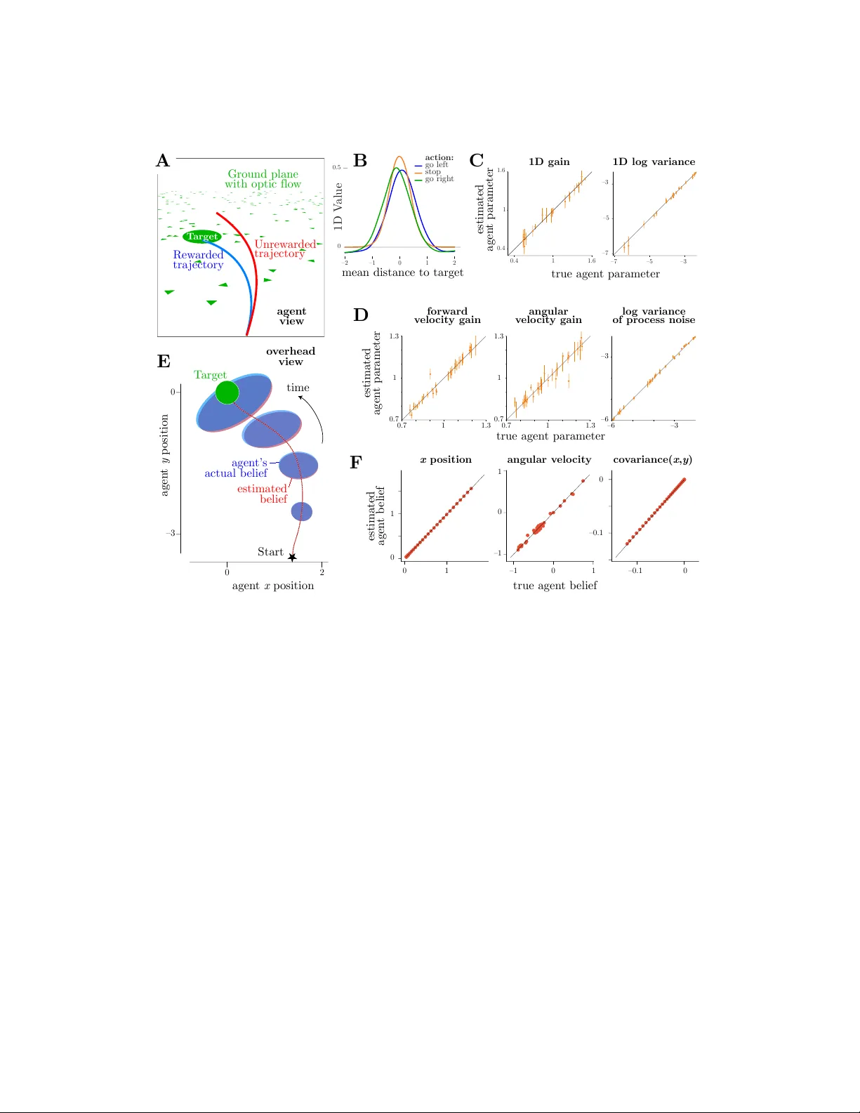
In verse Rational Contr ol with Partially Observ able Continuous Nonlinear Dynamics Saurabh Daptardar Department of ECE Rice Univ ersity Houston, TX 77005 svd3@rice.edu Paul Schrater Department of Computer Science Univ ersity of Minnesota Minnesota, IN 12345 schrater@umn.edu Xaq Pitkow Department of Neuroscience Baylor College of Medicine Houston, TX 77005 xaq@rice.edu Abstract Continuous control and planning remains a major challenge in robotics and machine learning. Neuroscience of fers the possibility of learning from animal brains that implement highly successful controllers, but it is unclear how to relate an animal’ s behavior to control principles. Animals may not always act optimally from the perspecti ve of an external observer , but may still act rationally: we hypothesize that animals choose actions with highest expected future subjective value according to their own internal model of the world. Their actions thus result from solving a different optimal control problem from those on which they are ev aluated in neuroscience experiments. W ith this assumption, we propose a novel frame work of model-based in verse rational control that learns the agent’ s internal model that best explains their actions in a task described as a partially observable Marko v decision process (POMDP). In this approach we first learn optimal policies generalized ov er the entire model space of dynamics and subjecti ve re wards, using an extended Kalman filter to represent the belief space, a neural network in the actor-critic framew ork to optimize the polic y , and a simplified basis for the parameter space. W e then compute the model that maximizes the likelihood of the experimentally observable data comprising the agent’ s sensory observations and chosen actions. Our proposed method is able to recover the true model of simulated agents within theoretical error bounds gi ven by limited data. W e illustrate this method by applying it to a complex naturalistic task currently used in neuroscience experiments. This approach pro vides a foundation for interpreting the beha vioral and neural dynamics of highly adapted controllers in animal brains. 1 Introduction Brains ev olved to understand, interpret, and act upon the physical world. T o thriv e and reproduce in a harsh and dynamic natural environment, animals therefore ev olved fle xible, robust controllers. Machine learning and neuroscience both aim to emulate or understand how these successful controllers operate. T raditional imitation learning or in verse control methods extract reusable policies to help generate autonomous behavior or help predict future actions from an agent’ s past behavior . In contrast, here we do not aim to extract the policy of a well-trained expert. Instead we want to identify the internal model and preferences of a real agent that may make interesting mistakes [ 13 ]. Unlike the con vention in robotics and artificial intelligence, animals are not optimized for stable, narrowly- defined tasks, but instead survive by performing well enough in competitiv e, changing ecological niches. Comparing actual control policies across conditions, animals, or species may ultimately guide us to broad control principles that generalize beyond specific tasks. Meanwhile, our approach Preprint. Under revie w . estimates latent assumptions and dynamic beliefs for real biological controllers, thereby pro viding targets for understanding neural network representations and implementations of perception and action. Our approach does not assume that agents perform optimally at a giv en task. Rather , we assume that agents are rational — by which we mean that agents act optimally according to their own internal model of the task, which may differ from the actual task. W e solve this problem by formulating the agent’ s policy as an optimal solution of a Partially Ob- servable Marko v Decision Process (POMDP) [ 20 ] that the agent assumes that it faces. Whereas Reinforcement Learning (RL) tries to find the optimal policy giv en the dynamics and the reward function, In verse Reinforcement Learning (IRL, [ 18 , 6 , 2 ]) tries to find a reward function which best accounts for observed actions from an agent. Similarly , in verse optimal control (IOC) [ 8 , 19 ] tries to find the assumed model dynamics that explains observed actions with a giv en cost function yields the similar optimal policy . Trying to find both is, in general, an ill-posed problem, but with a suf ficiently constrained model or proper conditioning it can be solved. Others have solved this problem in the fully observable setting [10, 17]. Some of the present authors recently solved the partially observ able case for a discrete state space with discretized beliefs [ 22 ]. Howe ver , while that solution was useful for their particular application, in general its computational e xpense grows rapidly with the problem complexity and size, and that solution assumes that actions are easy to select from the discretized value function. These issues makes that solution infeasible for continuous state spaces and continuous controls. In the present work, we provide methods that address these challenges. T wo major questions are ho w to construct representations of the agent’ s beliefs, and how to choose a policy based on those beliefs. W e solv e the first by assuming that agents kno w the basic task structure but not the task parameters, so we can use model-based inference to identify the agent’ s beliefs. W e solve the second by using flexible function approximation to estimate values and policies o ver the parameter space. W e demonstrate the utility of our approach by applying it to simulated agents in a continuous control task with latent variables that has been used in neuroscience: catching fireflies in virtual reality [13]. 2 Prior work on In verse Reinf orcement Lear ning In verse Reinforcement Learning (IRL) and In verse Optimal Control (IOC) solve aspects of the general problem of inferring internal models of an observed agent. Ng and Russell [ 15 ] formulate the IRL problem as a linear programming problem which takes agents policy as input and learn re ward parameters with an ` 2 regularization which makes the agent’ s policy optimal and also maximizes dif ference between the v alue at optimal action and v alue at next best action for each state (maximizing the margin of optimal polic y). Abbeel and Ng [ 1 ] extend the idea to perform maximum mar gin IRL. Max margin IRL introduces certain biases to solve the ambiguity of multiple reward functions. Some methods [ 23 ] resolve the ambiguity by adopting a principle of maximum entropy [ 11 ] to obtain a distribution o ver re ward functions without bias. Max Entropy IRL [ 23 ] tries to estimate a distribution ov er trajectories which has maximum entropy under the constraints of matching expectations of certain features. This approach is feasible only for finite discrete states and actions. and becomes intractable as the length of trajectories increases. For IOC, the Relati ve Entropy IRL frame work [ 5 ] allows for unkno wn dynamics, and minimizes the KL div er gence between two distributions o ver trajectories. The analytical solution needs a transition dynamics function which is estimated by importance sampling. It is important to note here that they do not assume the agent behaves optimally in an y sense. This method was extended in Guided Cost Learning by [ 9 ] to model a free maximum entropy formulation where the reward function is represented by a neural network. They use reinforcement learning to mov e the baseline policy tow ards policies with higher re wards imposing weak optimality . A more principled way to think about this problem class is to view the state action trajectories as observations about a re ward and dynamics with latent parameters [ 22 ]. [ 16 ] define the likelihood of trajectories as a e xponential Boltzmann distrib ution in state action v alue function Q ( s, a ; r ) . Their inference method performs a random walk o ver the re ward parameter space using the posterior , and compute the posterior ov er the parameters by computing the optimal action value function Q ∗ . This 2 is a nested loop approach that is feasible only for small spaces, as computing the optimal policy and value functions in the inner loop is costly . Other notable approaches include maximum likelihood IRL [ 21 , 2 ], Path Integral IRL [ 12 ], simultaneous estimation of rewards and fully-observed dynamics [ 10 ]. [ 12 ] proposes learning a continuous state, continuous action rew ard function by sampling locally around the optimal agent trajectories. These methods are local searches that do not consider trajectories with unexpected control input. Across all of these methods, there is not a complete inv erse solution that can learn ho w an agent models rew ards, dynamics, and uncertainty in a partially observable task with continuous nonlinear dynamics and continuous controls. 3 In verse Rational Control T o define the In verse Rational Control problem, we first formalize our tasks as Partially Observ able Markov Decision Processes (POMDPs). A POMDP M is a tuple, M = ( S, A, Ω , R, T , O, γ ) that includes states s ∈ S , actions a ∈ A , observations o ∈ Ω , rew ard or loss function R , as well as transition probabilities T ( s 0 | s, a ) , observation probabilities O ( o | s ) , and a temporal discount factor γ . Since the states s are only partially observ able, the POMDP determines the agent’ s time-dependent ‘belief ’ about the world, namely a posterior ov er states gi ven the history of observ ations and actions, b t = p ( s t | o 1: t , a 1: t ) . An optimal solution of the POMDP determines a value function Q ( b, a ) through the Bellman equation [ 4 ], which in turn defines a policy π that selects the action that maximizes the value. W e parameterize R , T and O , and therefore the value function and polic y , by θ = ( θ r , θ t , θ o ) . W e define the In verse Rational Control problem as identifying, using only data measurable from an agent’ s behavior , the most probable internal model parameters θ ∈ Θ for an agent that solves the POMDP described above. Specifically , we allow measurements of the states and action trajectory taken by the agent, but we have no access to the beliefs that motiv ate those actions. The agent’ s sensory observations may be fully observed, fully unobserved, or partially observed, for instance when we cannot access the particular observ ation noise that corrupts the agent’ s senses. A solution to IRC provides both parameters and an estimate of the agent’ s beliefs ov er time. A core idea in our approach is first to learn policies and value functions over the parameterized manifold of models, reflecting an optimized ensemble of agents, rather than a single optimized agent. This then allows us to maximize the likelihood of the observed data generated by an unknown agent, by finding which parameters from the ensemble best explain the agent’ s actions. Because our ov erarching goal is scientific, a major benefit of this approach is to provide the best interpretable explanation of an agent’ s behaviors as rational for a task as defined by some parameters θ . 3.1 General formulation of optimal contr ol ensembles There are two dif ficulties in solving the POMDP model ensemble and computing a lik elihood function ov er trajectories. First, policies and v alue functions are complex functions of the model parameters. W e address this by using flexible, trainable networks to learn the value function and policies, as described below . Second, the belief updating process of the agent inv olves a dif ficult integral and requires correct handling of the agent’ s observations. The agent does not observe the world states s , but gets partial observ ations o about them that induce a belief b t = p ( s t | o 1: t , a 1: t , θ ) . When the agent plans into the future, it does not know the future observ ations, so it must mar ginalize over them to predict the consequences of its actions a . If an agent were giv en the observ ations, future beliefs would be known, b ut when observ ations are unknown the agent has only a distribution o ver beliefs arising from an av erage transition probability ¯ T θ d between belief states, ¯ T θ d ( b 0 | b, a ) = R do T θ t ( b 0 | b, a, o ) O θ o ( o | a, b ) . The parameters of this average transition probability subsume the parameters from the transitions and observation functions, θ d = ( θ t , θ o ) . Once we hav e formulated the problem completely in terms of belief states, and identified a tractable finite representation of them, then we can use many of the tools dev eloped for fully observed Marko v Decision Processes (MDP). An agent chooses its actions based on these beliefs according to a policy π as a ∼ π ( a | b ) . An optimal policy is the one that produces the maximal (temporally discounted) e xpected future re ward, which 3 can be computed using the Bellman equation, Q π θ ( b, a ) = R θ r ( b, a ) + γ Z Z Z da 0 db 0 do 0 T θ t ( b 0 | b, a ) O θ o ( o | b, a ) π ( a 0 | b 0 ) Q π θ ( b 0 , a 0 ) (1) = R θ r ( b, a ) + γ Z Z da 0 db 0 ¯ T θ d ( b 0 | b, a ) π ( a 0 | b 0 ) Q π θ ( b 0 , a 0 ) (2) In practice we replace the full posterior b by a parametric form (such as a multiv ariate Gaussian) for which the transitions can be computed tractably , although this may introduce approximation errors. T o solv e the inv erse problem by inferring an agent’ s internal model that guides their actions, we be gin with the simple observation that the optimal policy π ∗ ( a | b ; θ ) and optimal state-action value function Q ∗ ( b, a ; θ ) function change depending on the dynamics and the rewards of the problem. That is, the optimal policy and state-action value function should implicitly be functions of the dynamics and re ward parameters. W e will mak e this e xplicit by assuming that the dynamics and the rew ard function are parameterized functions denoted by ¯ T θ d ( b 0 | b, a ) and R θ r ( b, a ) . W e choose this parametric form wisely to impose and exploit structure in the task. Although the parametric form for the dynamics and re ward may be simple or conv enient, the resultant dependence of Q π on these parameters is usually more complicated. Therefore we represent Q π by a flexible function class. This class could be a family of end-to-end trainable deep networks, for example, or a sum of basis functions as used in nonlinear support vector machines. W e may learn the Q θ using any of a v ariety of reinforcement learning methods. In our work we trained a function approximator using rew ards obtained by policies across many parameters θ sampled from a uniform prior on parameter space Θ , although a good prior o ver the parameters could make learning faster and more robust. The optimal policy is to pick the best actions according to the updated v alue function. The re wards obtained by these actions can then pro vide additional information about the v alue function, so we may repeat the abov e procedure iterati vely until the value function con verges. Howe ver , ev en choosing the best action from a gi ven Q π can be dif ficult. When there are few allo wed actions, then the policy is easy to implement: one simply exhaustiv ely e valuates Q π for all actions and picks the most valuable. When there is a continuum of actions, such that this approach is infeasible, then must choose another method to maximize v alue. Here we select actions by approximating the policy using an actor -critic method implemented by a supplemental network that is trained to optimize the value function by Deep Deterministic Policy Gradient (DDPG) [ 14 ], although we could also use other versions of Policy Iteration or Q -learning. Our algorithm for Policy Iteration across model space is gi ven belo w: Algorithm 1 Learning optimal value functions across parameter space Giv en a class of POMDP problems ov er parameter space Θ 1: Initialize a random policy π 2: repeat 3: Sample multiple θ ∼ U (Θ) and store in D θ 4: for all θ ∈ D θ do 5: Generate ( b, a ) trajectories τ using policy π θ and store in T 6: end for 7: Solve equation 2 for Q π 8: Improv e policy π using Q π by either  -greedy updates, softmax action selection [ 20 ], or policy gradient for continuous actions. 9: until policy π con ver ges 10: return π ∗ ← π 3.2 In verse Rational Contr ol from optimal contr ol ensembles No w that we have constructed an ensemble of approximately optimal policies over the task space, we now aim to reco ver the true parameters of an agent whose beha vior we observe. Specifically , we try to find parameters which maximize the likelihood of the agent’ s trajectories. For a gi ven θ ∈ Θ , we know the transition dynamics and ha ve already computed the optimal policy . 4 Giv en the observ able state and action trajectories indexed by i ∈ { 1 . . . N } , the log likelihood of the model parameters θ gi ven the e xperimental observations of one trajectory i is L i = log p ( s i 0: T , a i 0: T | o i 0: T , θ ) = log p ( s i 0 ) + X t log π ( a i t | b i t ( o i 0: t ) , θ ) + log p ( s i t +1 | a i t , s i t , θ ) (3) Note that this likelihood is conditioned on observations o , which the agent has but the external observer does not. When we do not have the observ ations but only state action sequence and the initial state, ideally we would marginalize the likelihood in equation 3 over all latent observ ation trajectories, like in traditional Expectation Maximization [ 7 ]. Here instead we use a hard E step, taking the maximum a posteriori (MAP) v alue for the observ ations given the observed state, ˆ o = argmax o O θ o ( o | s ) . T o maximize this likelihood, we rely on auto-dif ferentiation to compute the gradient of the polic y . The algorithm for learning the maximum likelihood estimate of true parameters giv en a state-action trajectory is giv en by Algorithm 2. Algorithm 2 Maximum Likelihood estimate for agent’ s parameters 1: Initialize θ randomly by sampling from the prior θ ∼ P (Θ) 2: repeat 3: Estimate agent’ s observations by MAP inference, ˆ o = argmax o O θ o ( o | s ) . 4: Estimate beliefs b giv en ˆ o using ˆ b t = p ( s t | ˆ o 1: t , a 1: t ) . 5: Compute total log-likelihood ov er trajectories L ← X i L i where L i is computed according to equation 3 6: Update θ by one gradient ascent step with learning rate α θ ← θ + α ∇ θ L 7: until L conv erges 8: return θ In Algorithm 1 we estimate optimal policies over the entire parameter space. When we then estimate the particular θ that best explains the agent’ s actions, it is by construction consistent with rational behavior: the best fit policy is optimal given those parameters, even if they do not match the actual task. Of course, for real data, this model fit does not imply that the agent’ s policy actually falls into our model class. Where needed, the model class should be expanded to accommodate other potentially false assumptions the agent may make. W e can summarize the whole In verse Rational Control framew ork in Algorithm 3: Algorithm 3 Parameter space In verse Rational Control 1: Define a family of POMDPs for the task, parametrized by Θ . 2: Learn the state-action value functions Q ( b, a ; θ ) o ver θ ∈ Θ using Algorithm 1. 3: Estimate agent’ s parameters ˆ θ from its observ able behavior using Algorithm 2. 4 Demonstration task: ‘Catching fireflies’ W e demonstrate that our proposed Inv erse Rational Control framew ork works by recoveri ng the internal model of simulated agents performing two control tasks. Ultimately we will apply this approach to understand the internal control models of behaving animals in neuroscience experiments, where we do not know the ground truth. Howe v er , using simulated agents allows us to verify the method when we know the ground truth. In this task, an agent must navigate through a virtual world to catch a flashing tar get, called the ‘firefly’ (Figure 1A) [ 13 ]. When the agent stops moving, the trial ends, the agent recei ves a re ward if it is sufficiently close to the firefly position, and a new tar get appears. Each target is visible only briefly , 5 and sensory inputs provide partial (noisy) observations of self motion, so the agent is uncertain about the current position of its target as well as its current v elocity . Unrew arded tra jectory Rew arded tra jectory T arget T arget forw ard v elo cit y gain agen t view A B C D E F o v erhead view estimated b elief time agen t’s actual b elief true agen t param eter true agen t param eter true agen t b elief agen t x p osition agen t y p osition es timated agen t param eter es timated agen t parameter estimated agen t b elief angular v elo cit y gain log v ariance of pro cess noise x p osition angular v elo cit y co v ariance( x , y ) 2 0 0 –3 Ground plane with optic flo w Start –3 –6 1 1.3 0.7 1 1.3 0.7 0.7 0 1 0 –0.1 –0.1 0 0 1 1 –1 –1 0 1 0 1 1.3 0.7 1 1.3 –6 –3 1D gain 1D log v ariance 1.6 1.6 0.4 0.4 1 –3 –7 –5 1 0 1 2 –2 0.5 0 –1 –7 –5 –3 go left action: s top go righ t m ean distance to target 1D V alue Figure 1: Firefly control task [ 13 ]. ( A ) T o reach the transiently visible firefly target, an agent must navigate by noisy optic flow o ver a dynamic textured plane. ( B ) For a 1D version of this task with only three allowed actions a , we deriv e sensible state-action value functions Q ( b, a ; θ ) , here showing that it is best to mov e tow ard the target and then stop, unless the tar get is too far to justify the ef fort. Our method accurately recov ers the agent’ s assumed parameters within limits imposed by the data, both for the 1D task ( C ) and the 2D task ( D ), as shown for several e xample parameters θ inferred from dif ferent agents. Error bars show 95% confidence interv als derived from the curvature of the likelihood gi ven limited data. ( E ) Overhead vie w illustrates one agent’ s belief dynamics, depicted by posterior cov ariance ellipses centered at each believ ed location (blue), as well as our method’ s estimates of those beliefs (red). ( F ) The estimated and true belief dynamics closely match. Three representativ e components of the belief representation are shown here: most likely firefly x position, most likely angular velocity , and the posterior co v ariance between x and y . The two e xample problems both use this task structure, either in one or two dimensions. In the 1D task, the world state and control variables are therefore location and forw ard velocity , and we only allow three discrete control outputs. In the 2D task we add angle and angular velocity to the state space, allo w continuous control outputs, and allow the agent to make noisy observations of its state. Giv en the uncertainty in its state estimate, the agent must track its belief ov er the states, and plan its optimal trajectory based on this belief state space and unknown future belief transitions based on unknown future observations. Given this task setting, the agent maximizes its reward e xpected ov er the distribution implied by the belief. Each episode or trial is a variable duration T depending on when the agent stops moving. The goal is to maximize the total rewards o ver this finite time horizon. Our first simulation experiment is a simplified version of the task, where the agent’ s position is restricted to one dimension, state dynamics are linear , and the agent receiv es no observ ations. The belief state is Gaussian-distributed o ver the agent’ s relativ e location to the target, with scalar mean µ 6 and variance σ 2 ev olving as µ t +1 = µ t + g a a σ 2 t +1 = σ 2 t + σ 2 0 (4) The model parameters are the action gain g a and the process noise log standard deviation log σ 0 . W e hav e only three discrete actions, namely: go left, go right, and stop. T o compute the optimal policies we use a Q -learning variant of Algorithm 1. Recall that we can substitute different learning algorithms, b ut it is crucial to learn the optimal action value function Q ∗ or policy as a function of θ . One approach we took for the 1D demonstration task was to construct Q from a factorized set of basis functions. W e experimented with both manually constructed polynomial and exponential basis functions, and a collection of random shallo w networks as basis functions for both φ ( b, a ) and ψ ( θ ) . W e found that the random network basis was more expressi ve and performed better for this task. Figure 1B plots the value function Q ∗ ( s, a, θ ) for each action and a fixed θ . Now that we ha v e computed the optimal policies ov er a manifold of parameters, we create an agent with one particular set of parameters θ ∗ . Using the corresponding opt imal policy and belief dynamics, we simulate this agent’ s belief state and action trajectories. Next we use experimentally observ able data (the action sequence) to update the belief trajectory per our model. Gi ven this data we follow the maximum likelihood estimation as described in Algorithm 2 using the most probable belief states to estimate the parameters. In Figure 1C we plot the estimated parameters recovered by our algorithm against the agent’ s true parameters, along with the 95% confidence interval for parameter θ i as giv en by 2( I − 1 / 2 ) ii where I is the Fisher information matrix. In almost all cases the true v alue is within the resultant error bars, sho wing that we correctly recover the true parameters within the precision allowed by the data. Our second simulation uses the full 2D firefly task. W e use two gain parameters, one on forward velocity input and another on angular v elocity input, and one process noise parameter that af fects x and y position identically , with no angular process noise. W e assume the agent maintains a Gaussian representation for its beliefs o ver the w orld state, which it updates using an e xtended Kalman filter giv en the dynamics parameters θ d . T o compute the optimal policies we use Deep Deterministic Policy Gradient (DDPG) [ 14 ] in Algo- rithm 1. W e sample the parameters uniformly o ver a moderate range and for each θ , we run the current policy π θ to collect sequences of belief states, actions, and rewards. Every time point ( ˆ b t , a t , r t ) in these sequences along with the corresponding θ was provided as input to two neural networks, each three layers deep, 64 units wide, and using softplus activ ations, whose output estimated the state-action value function and the policy . The learning updates for this are same as the DDPG algorithm. As before, we create an agent by choosing parameters θ ∗ , and generate trajectories using correspond- ing belief dynamics and optimal policy . W e preserve only the experimentally measurable action trajectories, and apply Algorithm 2 to compute the maximum likelihood estimate and confidence intervals. Figure 1D again shows that we can recover agents’ true parameters up to the intrinsic uncertainty . Additionally , we compare our estimates of their beliefs to their actual beliefs and find excellent agreement (Figure 1E,F). 5 Summary T o summarize our proposed in verse reinforcement learning framew ork, we express and learn the optimal action v alue function generalized ov er the task parameter space. This can be thought of as learning optimal v alue function and policy for all the parameters in the parameter space. For large, complex tasks, using an informativ e prior with sampling focused on relev ant regions of parameter space could greatly accelerate the learning and make the approximation more rob ust. Most other related frameworks ha ve a nested inner loop of policy optimization or refinement to adapt to the optimal policy for the ne w updated parameter . Unlike such methods, our method separates these optimizations into two separate loops, one for learning optimal policy over parameter space, and second for maximum likelihood estimation of the true parameters given the optimal policy computed in the previous loop. 7 5.1 Limitations Firstly , our assumption parametrized dynamics and rew ard function induces obvious model bias. Of course we can reduce this bias by making the parameter space richer and more flexible by increasing the number and variety of parameters. Howe v er , this would come with a price in computability and interpretability . In case of POMDPs, where we need to work with posterior distribution ov er the states or the belief, deriving analytical parametric belief update equations can be a difficult inference problem in general. For special cases like finite discrete states, the posterior updates can be succinctly represented matrix products, parameterized by transition matrices. For continuous state and Gaussian noises, we can use Kalman filter updates which are parameterized by the gain and cov ariance matrices, and for small nonlinearity this can be generalized using extended Kalman filters. But for general cases with general posterior distributions, a belief update might be a difficult inference problem. Though this is not necessarily a limitation of our approach but a challenge for inference problems more generally , still it may be difficult to apply our method in such cases. Similarly , as stated se veral times abo ve, the learning in Algorithm 1 can be replaced with an y suitable reinforcement learning algorithm which guarantees con v ergence to an optimal polic y , as long as the policy or the Q function is explicitly a function of model parameters. Our frame work theoretically does not limit the number of parameters as long as there is some algorithm which can e xplore and learn optimal policy o ver that lar ge space. 5.2 Outlook One interesting novelty of our framework is to make optimal action value Q ∗ and optimal policy π ∗ explicit functions of the parameters θ . W e can use this representation to extend the control task to hierarchical models: Instead of thinking of the parameters as fixed in the environment, we could consider them to be slo wly changing latent variables describi ng task demands in a dynamic world. The value function o ver this lar ger space would then pro vide a means of adapti ve control, where the agent could adjust its policy based on its current belief about θ . T o use IRC for such an agent, we would then need to introduce higher-le vel parameters that describe the full dynamics.No w , this looks like an y other optimal control problem, and when we solv e for optimal control problem for ˜ M as a function of augmented state ˜ s , we are learning the optimal control for M θ generalized ov er θ . W e ha ve implemented In verse Rational Control for neuroscience applications, but the core principles hav e value in other fields as well. W e can view IRC as a form of Theory of Mind, whereby one agent (a neuroscientist) creates a model of another agent’ s mind (for a behaving animal). Theory of Mind is a prominent component of social interactions, and imputing rational motiv ations to actions provides a useful description of how people think [ 3 ]. Designing useful artificial agents to interact with others in online en vironments would also benefit from being able to attrib ute rational strategies to others. One important example is self-driving cars, which currently struggle to handle the perceived unpredictability of humans. While humans do indeed behave unpredictably , some of this may stem from ignorance of the rational computation that drives actions. In verse Rational Control provides a frame work for better interpretation of other agents, and serves as a valuable tool for greater understanding of unifying principles of control. Acknowledgments The authors thank Kaushik Lakshminarasimhan, Dora Angelaki, Greg DeAngelis, James Bridgew ater and Minhae Kwon for useful discussions. SD and XP were supported in part by the Simons Collaboration on the Global Brain award 324143. PS and XP were supported in part by BRAIN Initiativ e grant NIH 5U01NS094368. XP was supported in part by an award from the McNair Foundation, NSF CAREER A ward IOS-1552868, and NSF 1450923 BRAIN 43092-N1. References [1] Pieter Abbeel and Andre w Y Ng. Apprenticeship learning via in verse reinforcement learning. In Pr oceedings of the twenty-first international confer ence on Machine learning , page 1. A CM, 2004. 8 [2] Monica Babes, V ukosi Mariv ate, Kaushik Subramanian, and Michael L Littman. Apprenticeship learning about multiple intentions. In Pr oceedings of the 28th International Conference on Machine Learning (ICML-11) , pages 897–904, 2011. [3] Chris Baker , Rebecca Saxe, and Joshua T enenbaum. Bayesian theory of mind: Modeling joint belief-desire attribution. In Pr oceedings of the annual meeting of the cognitive science society , volume 33, 2011. [4] R Bellman. Dynamic pr ogramming . Princeton Univ ersity Press, 1957. [5] Abdeslam Boularias, Jens Kober , and Jan Peters. Relati v e entropy in verse reinforcement learning. In Pr oceedings of the F ourteenth International Confer ence on Artificial Intelligence and Statistics , pages 182–189, 2011. [6] Jaedeug Choi and K ee-Eung Kim. In verse reinforcement learning in partially observable en vironments. Journal of Mac hine Learning Resear ch , 12(Mar):691–730, 2011. [7] Arthur P Dempster , Nan M Laird, and Donald B Rubin. Maximum likelihood from incomplete data via the em algorithm. Journal of the Royal Statistical Society: Series B (Methodological) , 39(1):1–22, 1977. [8] Krishnamurthy Dvijotham and Emanuel T odorov . In verse optimal control with linearly-solvable mdps. In Pr oceedings of the 27th International Confer ence on Machine Learning (ICML-10) , pages 335–342, 2010. [9] Chelsea Finn, Ser gey Le vine, and Pieter Abbeel. Guided cost learning: Deep in verse optimal control via policy optimization. In International Confer ence on Machine Learning , pages 49–58, 2016. [10] Michael Herman, T obias Gindele, Jörg W agner, Felix Schmitt, and W olfram Burgard. In verse reinforcement learning with simultaneous estimation of rewards and dynamics. In Artificial Intelligence and Statistics , pages 102–110, 2016. [11] Edwin T Jaynes. Information theory and statistical mechanics. Physical r evie w , 106(4):620, 1957. [12] Mrinal Kalakrishnan, Peter Pastor , Ludovic Righetti, and Stefan Schaal. Learning objecti ve functions for manipulation. In Robotics and Automation (ICRA), 2013 IEEE International Confer ence on , pages 1331–1336. IEEE, 2013. [13] Kaushik J Lakshminarasimhan, Marina Petsalis, Hyeshin Park, Gregory C DeAngelis, Xaq Pitko w , and Dora E Angelaki. A dynamic bayesian observ er model re veals origins of bias in visual path integration. Neur on , 2018. [14] T imothy P Lillicrap, Jonathan J Hunt, Alexander Pritzel, Nicolas Heess, T om Erez, Y uv al T assa, David Silv er , and Daan W ierstra. Continuous control with deep reinforcement learning. arXiv pr eprint arXiv:1509.02971 , 2015. [15] Andrew Y Ng, Stuart J Russell, et al. Algorithms for inv erse reinforcement learning. In Icml , pages 663–670, 2000. [16] Deepak Ramachandran and Eyal Amir . Bayesian in verse reinforcement learning. Urbana , 51(61801):1–4, 2007. [17] Siddharth Reddy , Anca D. Dragan, and Sergey Le vine. Where do you think you’ re going?: Inferring beliefs about dynamics from behavior . In Arxiv 1805.08010 , 2018. [18] Stuart Russell. Learning agents for uncertain en vironments. In Pr oceedings of the eleventh annual confer ence on Computational learning theory , pages 101–103. A CM, 1998. [19] Felix Schmitt, Hans-Joachim Bieg, Michael Herman, and Constantin A Rothkopf. I see what you see: Inferring sensor and policy models of human real-world motor behavior . In AAAI , pages 3797–3803, 2017. 9 [20] Richard S Sutton, Andrew G Barto, et al. Reinforcement learning: An intr oduction . MIT press, 1998. [21] Monica C Vroman. Maximum likelihood in verse r einfor cement learning . PhD thesis, Rutgers Univ ersity-Graduate School-Ne w Brunswick, 2014. [22] Zhengwei W u, Paul Schrater , and Xaq Pitko w . In verse POMDP: Inferring what you think from what you do. arXiv preprint , 2018. [23] Brian D Ziebart, Andre w L Maas, J Andrew Bagnell, and Anind K Dey . Maximum entropy in verse reinforcement learning. In AAAI , volume 8, pages 1433–1438. Chicago, IL, USA, 2008. 10