Adaptive Critic Based Optimal Kinematic Control for a Robot Manipulator

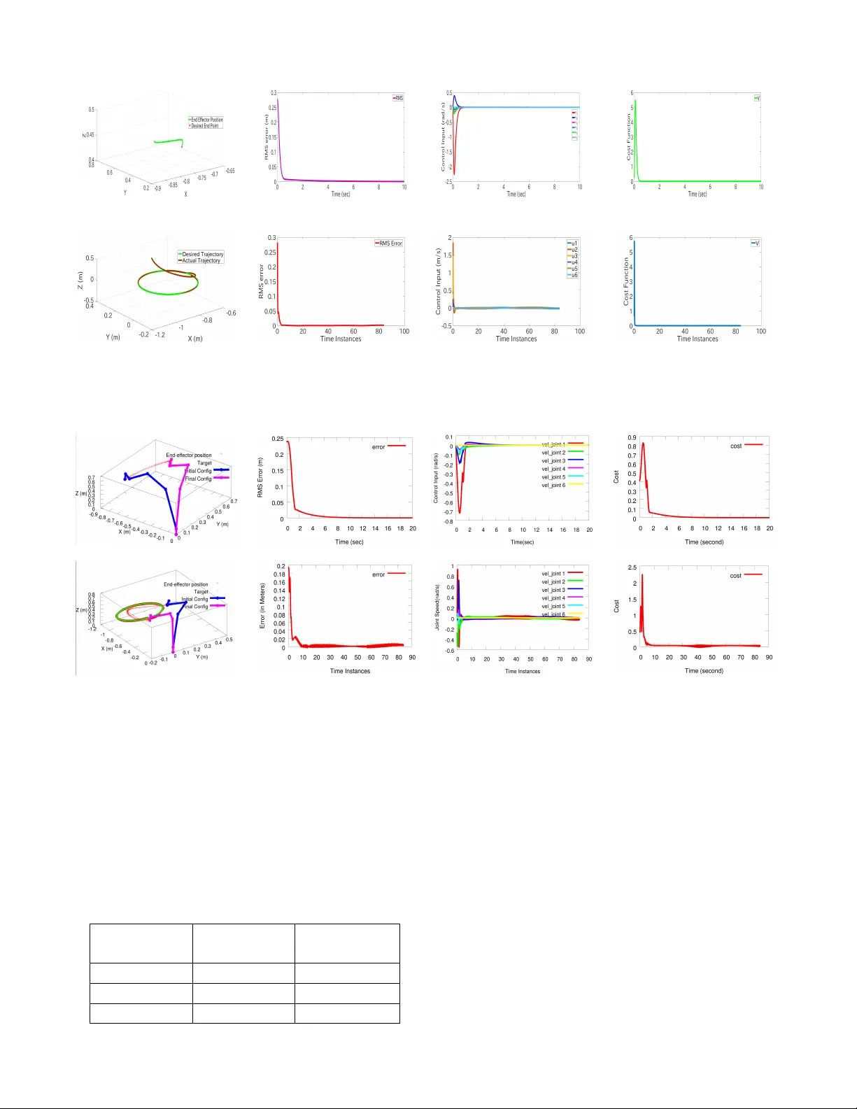
Adaptiv e Critic Based Optimal Kinematic Contr ol f or a Robot Manipulator Aiswarya Menon 1 , Ravi Prakash 2 , Laxmidhar Behera 3 , Senior Member , IEEE Abstract — This paper is concerned with the optimal kine- matic control of a r obot manipulator where the r obot end effector position follo ws a task space trajectory . The joints are actuated with the desired velocity profile to achieve this task. This problem has been solved using a single network adaptive critic (SNA C) by expr essing the f orward kinematics as input affine system. Usually in SNA C, the critic weights ar e updated using back propagation algorithm while little attention is given to con vergence to the optimal cost. In this paper , we propose a critic weight update law that ensures con vergence to the desired optimal cost while guaranteeing the stability of the closed loop kinematic control. In kinematic contr ol, the robot is requir ed to reach a specific target position. This has been solved as an optimal r egulation problem in the context of SNA C based kinematic control. When the robot is required to follo w a time varying task space trajectory , then the kinematic control has been framed as an optimal tracking problem. For tracking, an augmented system consisting of tracking error and reference trajectory is constructed and the optimal control policy is derived using SNA C framework. The stability and performance of the system under the pr oposed novel weight tuning law is guaranteed using L yapunov approach. The proposed kinematic control scheme has been validated in simulations and experimentally executed using a real six degrees of freedom (DOF) Universal Robot (UR) 10 manipulator . I . I N T RO D U C T I O N Modern robotic systems are becoming complex as the degrees of freedom are increasing to address the complex application scenario such as agriculture, health-care and ware-house automation. A mobile manipulator with Shadow hand mounted on it has 28 degrees of freedom. The in verse kinematic solution to such systems can not be solved analyt- ically . Thus neural and fuzzy neural network based schemes hav e become popular to design kinematic control[1], [2], [3], [4]. These approaches can not learn the in verse kinematics while optimizing a global cost function. This is very im- portant when one deals with redundant manipulators. One of the approaches to design optimal kinematic control is to use the Hamilton-Jacobi-Bellman (HJB) formulation [5], [6]. The analytical solution of the HJB equation is still a major challenge and as such these solutions are obtained off-line. The real time approximate solutions are known as approximate dynamic programming and are presented in [7], [8], [9]. In these approaches, the framework uses two neural networks - one for action and the other critic. Action network learns to actuate an optimal policy while critic netw ork ev aluates the cost function through learning. All authors are with the Department of Electrical Engineering, Indian Institute of T echnology , Kanpur, India-208016. Email id : 1 aiswarya@iitk.ac.in, 2 ravipr@iitk.ac.in, 3 lbehera@iitk.ac.in The single network adaptiv e critic (SN AC) is introduced [10] where critic is updated using back-propagation. In Fig. 1: Block diagram of the kinematic control scheme for a robot manipulator using adaptive critic method [11], the kinematic control of a robot manipulator using this SN AC framew ork was presented. The block diagram of the kinematic control scheme for a robot manipulator using SN AC is shown in Fig. 1. As these schemes used back-propagation for critic weight updates, after repeated training, one could show the con vergence to near optimal cost through extensi ve simulations. There exists very few works in the literature that has shown the con vergence to the optimal cost in an analytical manner along with the proof of stability . In this work, we are solving the kinematic control problem of any n -DOF robot manipulator where the tasks of reaching a fixed target position and following a time varying task space trajectory hav e been solved in the frame work of optimal regulation and optimal tracking respectiv ely using SN A C. A simple and nov el critic weight update rule which ensures that the closed loop system is stable has been proposed. The optimal kinematic control policy using HJB formulation has been developed in the framew ork of optimal regulation and optimal tracking. Former make the robot to reach fixed target position and later make the robot to follo w the task-space time varying trajectory . The analytical proof of stability and con vergence has been done using L yapunov approach. As the degrees of freedom of robotic systems are increasing, learning based strategies wil l play more important role as compared to model based analytics [12],[13]. Thus the proposed approach has significant relev ance in this context. The relev ant literature is further scrutinized. The optimization based kinematic control has been accom- plished using local optimization for finding an instantaneous optimal solution [14], [15]. It is centered on the Jacobian pseudo-in verse and null space. The redundancy is resolv ed by including some constraints into the direct kinematic model or by projecting a particular solution onto the Jacobian null space. The other approach is a global optimization which uses an integral type performance index along the whole trajectory [16], [17]. The redundancy resolution is conv erted to an optimal control problem with the necessary conditions of optimality giv en by the Pontryagin’ s principle or by the optimal control theory . Both of the aforementioned methods are suboptimal and require the pseudo-inv ersion of Jacobian continuously over time which is computationally expensi ve and suffers from local instability problems [18], [19], [20]. Existing approach to wards follo wing a time varying task space trajectory optimally is to find the feedforward term using the dynamics in version concept and the feedback term by solving an HJB equation [21]. Howe ver , such solution is only near optimal because of the feedforward term. There- fore by using an augmented system dynamics consisting of feedback tracking error and reference trajectory and using it to solve the HJB equation results in an optimal control law which is a combination of feedforward and feedback control inputs [22]. The remainder of this paper is organised as follows. Prob- lem formulation for optimal kinematic control is presented in Section II. In Section III and IV detailed mathematical deriv ation for the control scheme along with stability proof is presented. In Section V , various simulation and experimental results for kinematic motion control of a 6-DOF robotic manipulator are e valuated with comparison with the state- of-the-art kinematic control solutions. This paper is finally concluded in Section VI. I I . P RO B L E M F O R M U L A T I O N The forward kinematics of a manipulator in volv es a non- linear transformation from Joint space to Cartesian space as described by: x ( t ) = f ( θ ( t )) (1) where, x ( t ) ∈ R n × 1 describes the position and orientation of end effector in workspace at time t , θ ( t ) ∈ R m × 1 each element of which describes the joint angle in the joint space at time t , and f ( . ) is the non linear mapping. Because of non- linearity and redundancy of mapping, it is usually difficult to directly get θ ( t ) for desired x ( t ) = x d ( t ) , where x d ( t ) is the desired end effector position. By contrast, the mapping from joint space to cartesian space at velocity lev el is af fine mapping. T aking time deriv ativ e on both sides of (1) giv es: ˙ x ( t ) = J ˙ θ ( t ) (2) where, J = ∂ f ∂ θ ∈ R n × m is the Jacobian matrix of f ( . ) . In this paper we focus on design of angular speed of the manipulator which serves as an input to the tracking control loop for robot control. Then the robot manipulator kinematics can be rewritten by replacing ˙ θ ( t ) by u ( t ) : ˙ x ( t ) = J u ( t ) (3) Thus, we get the dynamics of the system as above. In this paper we propose to solve for an optimal control input u ( t ) for a robot manipulator described by (3), such that the tracking error giv en by , e ( t ) = x ( t ) − x d ( t ) (4) for a given reference trajectory x d ( t ) , reduces to zero with time. I I I . O P T I M A L R E G U L A T I O N In this section, we address the optimal kinematic control of a robot manipulator, where the robot end effector has to reach a fixed target position. This is framed as an optimal regulation problem. In the conte xt of kinematic control, optimal regulation means that the robot is made to reach a fixed target position following an optimal trajectory . This trajectory is generated by actuating the desired optimal control policy . Let x d ( t ) ∈ R n × 1 be the desired end effector position. Differentiating (4) with respect to time, error dynamics of the system is obtained as, ˙ e = ˙ x ( t ) = J u ( t ) (5) A. F ormulation of control policy The infinite horizon HJB cost function for (5) is gi ven by , V ( e ( t )) = ˆ ∞ t e ( t ) T Qe ( t ) + u ( t ) T Ru ( t ) dt (6) where, Q ∈ R n × n and R ∈ R m × m are positiv e definite design matrices. The control input needs to be admissible so that the cost function equation (6) is finite. The Hamiltonian for the this cost function with the admissible control input u ( t ) is, H ( e ( t ) , u ( t ) , ∇ V ( t )) = ∇ V ∗ T ˙ e ( t ) + e ( t ) T Qe ( t ) + u ( t ) T Ru ( t ) (7) Here, ∇ V ∗ is the gradient of the cost function V ( e ( t )) with respect to e ( t ) . The optimal control input which minimizes the cost function (6) also minimizes the Hamiltonian (7). Therefore, the optimal control is found by solving the following condition ∂ H ( e,u, ∇ V ) ∂ u = 0 and obtained to be u ∗ ( e ) = − 1 2 R − 1 J T ∇ V ∗ ( e ) (8) Then, HJB equation may be re-written as follows, 0 = ∇ V ∗ T ˙ e ( t ) + e ( t ) T Qe ( t ) + u ∗ ( t ) T Ru ∗ ( t ) (9) with the cost function V ∗ (0) = 0 . B. Neur al Network contr ol design By using the univ ersal approximation property , V ∗ ( e ( t )) is constructed by a single hidden layer neural network with a non-linear activ ation function: V ∗ ( e ( t )) = W T c σ c ( e ) + ε c (10) where, W c ∈ R l , is the constant target NN weight vector , σ c ∈ R l is the activ ation function output, l is the number of hidden neurons and ε c is the function reconstruction error . The target NN vector and reconstruction errors are assumed to be upper bounded according to k W c k≤ λ W c and k ε c k≤ λ ε . ∇ V ∗ = ∇ σ T c W c + ∇ ε c (11) Approximate optimal cost function and its gradient is giv en by ˆ V ∗ = ˆ W c T σ c ( e ) (12) ∇ ˆ V ∗ = ∇ σ T c ˆ W c (13) where, ˆ W c is the NN estimate of tar get weight vector W c . Using (8) and (11), the optimal control la w can be written as: u ∗ ( e ) = − 1 2 R − 1 J T ( ∇ σ T C W c + ∇ ε c ) (14) Considering (8) and (13), estimated optimal control law is: ˆ u ∗ ( e ) = − 1 2 R − 1 J T ∇ σ T c ˆ W c (15) The modified error dynamics using (15) is, ˙ e = − 1 2 J R − 1 J T ∇ σ T c ˆ W c (16) Before proposing the critic weight tuning law and stability proofs, following assumptions need to be made: Assumption 1: For the system represented by its error dy- namics (5), with cost function (6), let J s ( e ) be a continuously differentiable L yapunov function candidate satisfying, ˙ J s ( e ) = ∇ J s ( e ) T ˙ e < 0 (17) Then, there exists a positi ve definite matrix, M ∈ R n × n ensuring, ∇ J s ( e ) T ˙ e = −∇ J s ( e ) T M ∇ J s ( e ) ≤ − λ min ( M ) k ∇ J s ( e ) k 2 (18) During the implementation, J s ( e ) can be obtained by selecting a polynomial with respect to the vector e , such as J s ( e ) = 1 2 e T e . Remark 1 : Based on the result of [23], the closed loop dynamics with optimal control law can be bounded by a function of the system state. In such situations, it can be asssumed that k F ( e ) + G ( e )( u ∗ ) k≤ η k ∇ J s ( e ) k with η > 0 , k ∇ J s ( e ) k T k F ( e ) + G ( e )( u ∗ ) k≤ η k ∇ J s ( e ) k 2 . Combining (17) with the fact gi ven, λ min k ∇ J s ( e ) k 2 ≤ ∇ J s ( e ) T M ∇ J s ( e ) ≤ λ max ( M ) k ∇ J s ( e ) k 2 , it implies that assumption 1 holds. Moving on, a simple and no vel critic weight tuning law is proposed. ˙ ˆ W c = α ∇ σ c J R − 1 J T ∇ J s ( e ) (19) where, α is the learning rate of critic network and J s ( e ) = 1 2 e T e .By using this weight tuning law , stability and per- formance is guaranteed theoretically using the L yapunov approach. C. Stability Analysis In this section, the stability of the system for optimal regulation is inv estigated. Assumption 2 : The Jacobian matrix is bounded as k J ( θ ) k≤ λ J ,where λ J is a positive constant. Here, the control coef- ficient matrix is the Jacobian matrix. Also, ∇ σ c , ∇ ε c are bounded as k ∇ σ c k≤ λ σ and k ∇ ε c k≤ λ ∇ ε where λ σ and λ ∇ ε are positiv e constants. The L yapunov candidate function is selected as, L ( t ) = 1 4 α f W c T f W c + J s ( e ) (20) ˙ L ( t ) = 1 2 α f W c T ˙ f W c + ∇ J T s ˙ e (21) where, f W = W c − ˆ W c . Using (19), ˙ L ( t ) = − 1 2 f W c T ∇ σ J R − 1 J T ∇ J s + ∇ J T s ( ˙ e ) (22) The system error dynamics of the system for the optimal control law is ˙ e ∗ = J u ∗ . Using the control laws (14) and (15), ˙ e ∗ − ˙ e = J ( u ∗ − ˆ u ∗ ) = − 1 2 J R − 1 J T ( ∇ σ T c f W c + ∇ ε c ) (23) Using (23) in (22) and on simplification, ˙ L ( t ) = ∇ J T s ˙ e ∗ + 1 2 ∇ J T s J R − 1 J T ∇ ε c (24) Applying Assumption 1 and Assumption 2 here ˙ L ≤ − λ min ( M ) k ∇ J s k 2 + 1 2 k ∇ J s k λ 2 J k R − 1 k λ ∇ ε (25) From (25), the following inequality may be deriv ed: k ∇ J s k≥ 1 2 λ min ( M ) λ 2 J k R − 1 k λ ∇ ε (26) W ith the above condition to be true, ˙ L ≤ 0 and the system is stable in the sense of L yapunov implying that f W c and e are both bounded. It may be expressed as : k f W c k≤ λ f W c . It may be also observ ed that the estimated optimal con- troller (15) con verges to a neighborhood of the optimal feedback controller (14) with a finite bound λ u as, k u ∗ ( e ) − ˆ u ∗ ( e ) k≤ 1 2 k R − 1 k λ J ( λ σ λ f W c + λ ∇ ε ) ∆ = λ u (27) Hence, it may be concluded that the instantaneous cost function V ( e, u, t ) = e ( t ) T Qe ( t ) + u ( t ) T Ru ( t ) is also bounded. T aking time deriv ativ e of (24), ¨ L = ˙ e T ˙ e ∗ + e T ¨ e ∗ + 1 2 ˙ e T J R − 1 J T ∇ ε c + e T ˙ J R − 1 J T ∇ ε c + 1 2 e T J R − 1 J T ∇ 2 ε c ˙ e (28) Remark 2: All the terms in ¨ L can be shown to be bounded. It may be observ ed that ¨ L is bounded and Barbalat’ s Lemma [24] can be in voked to conclude the asymtotic stability of the system and con ver gence of the parameter estimation error and the weight estimation errors towards zero. In other words, it ensures that f W c → 0 . I V . O P T I M A L T R AC K I N G C O N T RO L In this section, the kinematic control of a robot manipula- tor following a time v arying task space trajectory is solved in the framew ork of optimal tracking. A. F ormation of Augmented System Let the time varying reference trajectory , denoted by x d ( t ) ∈ R n be possessing the dynamics ˙ x d ( t ) = ϕ ( x d ( t )) (29) with the initial condition x d (0) = x d 0 , where, ϕ ( x d ( t )) is a Lipschitz continuous function satisfying ϕ (0) = 0 . Let the trajectory tracking error be e ( t ) = x ( t ) − x d ( t ) with the initial condition e (0) = e 0 = x 0 − x d 0 . Considering (3) and (29), the tracking error dynamics is: ˙ e ( t ) = − ϕ ( x d ( t )) + J u ( t ) (30) Next, an augmented system is constructed as in [22],in the form ξ ( t ) = [ e ( t ) T , x d ( t ) T ] T ∈ R 2 n with initial condition ξ (0) = ξ 0 = [ e T 0 , x d T 0 ] T . The augmented dynamics based on (29) and (30) can be formulated as: ˙ ξ ( t ) = F ( ξ ( t )) + G ( ξ ( t )) u ( t ) (31) where, F(.) and G(.) are the new system matrices. B. F ormulation of Control P olicy The infinite horizon HJB cost function for the system in (31) is giv en by , V ( ξ ( t )) = ˆ ∞ t ξ ( t ) T ¯ Qξ ( t ) + u ( t ) T Ru ( t ) .dt (32) where, ¯ Q = diag { Q, 0 n × n } . Q ∈ R n × n and R ∈ R m × m are positive definite matrices. The control input must be admissible so that cost function given by (32) is finite. Applying the same methods of solving as in Section III-A, the control policy is obtained as, u ∗ ( ξ ) = − 1 2 R − 1 G ( ξ ) T ∇ V ∗ ( ξ ) (33) C. Neur al Network contr ol design Here, V ∗ ( ξ ( t )) is constructed by a single hidden layer neural network with a non-linear activ ation function: V ∗ ( ξ ( t )) = W T c φ c ( ξ ) + ε c (34) where, W c ∈ R p , is the ideal weight, k W c k≤ λ W c , φ c ∈ R p is the activ ation function output, p is the number of hidden neurons and ε c is the function approximation error . Using the same approach as in Section III-B, optimal control law and approximate control law may be obtained as, u ∗ ( ξ ) = − 1 2 R − 1 G ( ξ ) T ( ∇ φ T C W c + ∇ ε c ) (35) ˆ u ∗ ( ξ ) = − 1 2 R − 1 G ( ξ ) T ∇ φ T c ˆ W c (36) Applying (36) into the augmented system dynamics (31), ˙ ξ ( t ) = F ( ξ ) + G ( ξ ) ˆ u ∗ ( t ) can be formulated as: ˙ ξ = F ( ξ ) − 1 2 G ( ξ ) R − 1 G ( ξ ) T ∇ φ T c ˆ W c (37) The weight update law proposed for the critic of optimal tracking control is, ˙ ˆ W c = α ∇ φ c G ( ξ ) R − 1 G ( ξ ) T ∇ J s ( ξ ) (38) where, α is the learning rate of critic network and J s ( ξ ) = 1 2 ξ T ξ . Remark 3: Assumption 1 and Remark 1 holds here. The augmented system states shall replace the system error states as follows ; For the augmented system (31), with cost function (32), let J s ( ξ ) be a continuously differentiable L yapunov function candidate satisfying, ˙ J s ( ξ ) = ∇ J s ( ξ ) T ˙ ξ < 0 (39) Then,there exists a positi ve definite matrix, M ∈ R 2 n × 2 n ensuring, ∇ J s ( ξ ) T ˙ ξ = −∇ J s ( ξ ) T M ∇ J s ( ξ ) ≤ − λ min ( M ) k ∇ J s ( ξ ) k 2 (40) During the implementation, J s ( ξ ) = 1 2 ξ T ξ . D. Stability Analysis In this section, the stability of the system is in vestigated. Remark 4 : Assumption 2 holds here. Howe ver , the control coefficient matrix is modified. The assumption k G ( ξ ) k≤ λ g , where λ g is a positiv e constant shall be used. L yapunov function, L ( t ) = 1 4 α f W c T f W c + J s ( ξ ) (41) ˙ L ( t ) = 1 2 α f W c T ˙ f W c + ∇ J T s ˙ ξ (42) Using the similar approach as in Section III-C, ˙ L ( t ) = ∇ J T s ˙ ξ ∗ + 1 2 ∇ J T s G ( ξ ) R − 1 G ( ξ ) T f W c (43) Applying the Remark 3 and Remark 4 here ˙ L ≤ − λ min ( M ) k ∇ J s k 2 + 1 2 k ∇ J s k λ 2 g k R − 1 k λ ∇ ε (44) From this, we observe that if the condition below holds, then, ˙ L ( t ) ≤ 0 is negati ve semidefinite implying that the system is stable in the sense of L yapunov . k ∇ J s k≥ 1 2 λ min ( M ) λ 2 g k R − 1 k λ ∇ ε (45) Hence, f W c and ξ are both bounded. It may be expressed as : k f W c k≤ λ f W c Also, k u ∗ ( ξ ) − ˆ u ∗ ( ξ ) k≤ 1 2 k R − 1 k λ g ( λ σ λ f W c + λ ∇ ε c ) ∆ = λ u (46) It may be noted that estimated controller input conv erges to the neighbourhood of the optimal control input as a finite bound λ u exists just as in the case of regulation. It is also observed that the cost function V ( ξ , u, t ) = ξ ( t ) T ¯ Qξ ( t ) + u ( t ) T u ( t ) is also bounded. Using the same approach as in Section III-C, it may be sho wn that ¨ L is bounded. Recalling Barbalat’ s Lemma [25], it may be concluded that the system is stable and that the parameter estimation error and weight estimation error con verge to zero. Fig. 2: Hardware Setup V . R E S U LT S A N D D I S C U S S I O N In this section, we consider the numerical simulations fol- lowed by real time experimental validations on a real 6 DOF UR 10 robot manipulator to demonstrate the ef fecti veness of the proposed kinematic control. A. Experimental Setup Our experimental setup shown in Fig. 2 consists of a UR10 robot manipulator with its controller box/internal computer and a host PC/external computer . The UR10 robot manipulator is a 6 DOF robot arm designed to safely work alongside and in collaboration with a human. This arm can follow position commands like a traditional industrial robot, as well as take velocity commands to apply a giv en velocity in/around a specified axis. The low level robot controller is a program running on UR10’ s internal computer broadcasting robot arm data , receiving and interpreting the commands and controlling the arm accordingly . There are sev eral options for communicating with the robot low lev el controller to control the robot including the teach pendent or opening a TCP socket (C++/Python) on a host computer . W e used open source C++ based UrDriv er wrapper class integrated with R OS on a host PC to implement our proposed velocity based kinematic control scheme. The host PC streams joint velocity commands via URScript to the robot real time interface ov er Ethernet at 125 H z . The dri ver w as configured with necessary parameters like IP address of the robot at startup using ROS parameter server . B. Reac hing a F ixed P osition Simulations are first performed to verify the kinematic control of the robot manipulator to reach a fixed position using the control law expressed in Equation (15). A typical simulation run generated with a random seed pose ( θ 0 = [ − 0 . 51 − 1 . 041 . 48 − 1 . 82 − 1 . 45 − 1 . 62] r ad ) to a fixed target pose [ − 0 . 658 , 0 . 626 , 0 . 407] m in cartesian space is sho wn in Figure 3(a).The weights were initialized randomly and α = α initial ( tanh ( n − k ))+ α f inal , where, n=50, k=time instance, α initial = 100 and α f inal = 150 .The predicted cost function was: w 1 e 2 1 + w 2 e 1 e 2 + w 3 e 1 e 3 + w 4 e 2 2 + w 5 e 2 e 3 + w 6 e 2 3 C. F ollowing a T ime V arying Refer ence T rajectory In this section, the kinematic control of the robot ma- nipulator to follow a time varying reference trajectory is validated. Simulations are first performed using the control law derived in Equation (36). A typical simulation generated with a random seed pose ( θ 0 = [ − 0 . 51 − 1 . 041 . 48 − 1 . 82 − 1 . 45 − 1 . 62] r ad ) and following a time v arying reference trajectory moving at an angular speed of 0 . 075 r ad/s along a circle centered at [ − 0 . 7 , 0 , 0 . 5] m with a radius of 0 . 2 m is shown in Figure 3(e). W eights were initialized randomly and α = α initial ( tanh ( n − k )) + α f inal , where, n=10, k=time intance, α initial = 20 and α f inal = 70 . In this work, we take the predicted cost to be: w 1 ξ 2 1 + w 2 ξ 1 ξ 2 + w 3 ξ 1 ξ 3 + w 4 ξ 1 ξ 4 + w 5 ξ 1 ξ 5 + w 6 ξ 1 ξ 6 + w 7 ξ 2 2 + w 8 ξ 2 ξ 3 + w 9 ξ 2 ξ 4 + w 10 ξ 2 ξ 5 + w 11 ξ 2 ξ 6 + w 12 ξ 2 3 + w 13 ξ 3 ξ 4 + w 14 ξ 3 ξ 5 + w 15 ξ 3 ξ 6 + w 16 ξ 2 4 + w 17 ξ 4 ξ 5 + w 18 ξ 4 ξ 6 + w 19 ξ 2 5 + w 20 ξ 5 ξ 6 + w 21 ξ 2 6 . D. Observations After a short transient time, the error trajectory e ( t ) = x ( t ) − x d ( t ) con verges to zero in both cases as shown in Fig. 3(b) and 3(f) respectiv ely . Note that the control input u = ˙ θ remain within the maximum joint velocity limits sho wn in Fig. 3(c) and Fig. 3(g). Ho wever unlik e in optimal re gulation, it does not conv erge to zero as the velocity compensation is required for perfect tracking control. The time history plot of the associated cost function is shown in shown in Fig. 3(d,h). The e xperimental v alidation for the corresponding tar get pose was performed using a real UR 10 robot manipulator . The results from Fig. 4 shows that the end effector of UR 10 robot manipulator successfully reaches the target pose under the proposed control scheme and successfully follows the reference time varying circular trajectory starting from a random seed pose. The time history plot of the associated cost function is shown in Fig. 4(d,h). Unlike in simulations, the control effort sho ws some chatter due to the inertia of the real hardware. E. Quantitative T est Comparison In order to quantify the performance of the proposed optimal kinematic control, an automated test process was used where a large, statistically-valid number of random samples were used as inputs. Kinematic models of Universal Robot (UR) 10 was used to demonstrate the tests. The quantitativ e test methodology for comparing the proposed method for kinematic control against the state-of-the-art kinematic control using an RNN [ 3 ] and Singluar V alue Filtering (SVF) approach [26] is entailed. First, a total of 1 , 000 random samples and 1000 dif- ferent feasible elliptical trajectories were generated in the sample space for regulation and tracking respectively . The sample space is a cuboid volume of task space within robot’ s reach and every sample is a pair of seed pose and target pose in the case of regulation. The three kinematic (a) (b) (c) (d) (e) (f) (g) (h) Fig. 3: Simulation results for Optimal regulation of a fixed target (a-d) and optimal tracking for a time varying elliptical trajectory (e-h). (a) (b) (c) (d) (e) (f) (g) (h) Fig. 4: Experimental results for Optimal regulation of a fixed target (a-d) and optimal tracking for a time varying elliptical trajectory (e-h). control schemes mentioned above are tested and compared on trajectory cost. The trajectory cost is defined as nor- malized total cost: V / N , where V = ´ ∞ t e ( t ) T Qe ( t ) + u ( t ) T Ru ( t ) + ˙ u ( t ) T R ˙ u ( t ) dt for the same Q = I 3 × 3 and R = I 6 × 6 and N is the number of total sample instances. The design parameters were selected such that the maximum control effort is the same for all three approaches. Controller T rajectory cost T rajectory Cost Regulation T racking Controller [3] 49 . 74 14 . 39 Controller [26] 48 . 32 32 . 21 Proposed 5 . 78 3 . 30 T ABLE I: Comparisons of different algorithms for Kinematic Control of UR10 Robot Manipulator The cost matrix contain two terms. One for the measure of optimal control action and another for smoothness of the motion. The comparison from T able I sho ws that the proposed kinematic control has the optimal control action than the state-of-the-art kinematic control. V I . C O N C L U S I O N In this work, we have designed an optimal kinematic con- troller for a robot manipulator using SN AC framew ork. A simple critic weight update law was proposed which ensured that the closed loop system becomes stable in the sense of L yapunov while follo wing an optimal trajectory . The robot was expected to reach a target position or follow a time v arying trajectory in the task space while optimizing a global cost function. Using the proposed optimal regulation and optimal tracking framew ork in the context of SNA C, it has been experimentally demonstrated that robot performs desired tasks with optimal cost as evident from T able 1. R E F E R E N C E S [1] S. Kumar , L. Behera, and T . McGinnity , “Kinematic control of a redundant manipulator using in verse-forward adaptive scheme with a ksom based hint generator , ” Robotics and Autonomous Systems , vol. 58, no. 5, pp. 622–633, 2010. [2] P . Prem Kumar and L. Behera, “Visual servoing of a redundant manipulator with jacobian matrix estimation using self-organizing map, ” Robotics and Autonomous Systems , vol. 58, no. 8, pp. 978–990, 2010. [3] S. Li, Y . Zhang, and L. Jin, “Kinematic control of redundant manipu- lators using neural networks, ” IEEE transactions on neural networks and learning systems , vol. 28, no. 10, pp. 2243–2254, 2017. [4] I. Sirazuddin, L. Behera, T . McGinnity , and S. Coleman, “Image based visual servoing of a 7 dof robot manipulator using an adaptive distributed fuzzy pd controller , ” IEEE/ASME T rans on Mechatr onics , vol. 19, no. 2, pp. 512–523, 2014. [5] F . L. Lewis, D. Vrabie, and V . L. Syrmos, Optimal contr ol . John W iley & Sons, 2012. [6] S. Keerthi and E. Gilbert, “ An existence theorem for discrete-time infinite-horizon optimal control problems, ” IEEE T ransactions on Automatic Contr ol , vol. 30, no. 9, pp. 907–909, 1985. [7] D. P . Bertsekas, D. P . Bertsekas, D. P . Bertsekas, and D. P . Bertsekas, Dynamic pr ogramming and optimal contr ol . Athena scientific Bel- mont, MA, 2005, vol. 1, no. 3. [8] Z. Chen and S. Jagannathan, “Generalized hamilton–jacobi–bellman formulation-based neural network control of affine nonlinear discrete- time systems, ” IEEE T ransactions on Neural Networks , vol. 19, no. 1, pp. 90–106, 2008. [9] J. Si, A. Barto, W . Powell, and D. W unsch, “Handbook of learning and approx. dynamics prog, ” 2004. [10] R. Padhi, N. Unnikrishnan, X. W ang, and S. Balakrishnan, “ A single network adapti ve critic (snac) architecture for optimal control synthesis for a class of nonlinear systems, ” Neural Networks , vol. 19, no. 10, pp. 1648–1660, 2006. [11] P . K. Patchaikani, L. Behera, and G. Prasad, “ A single network adaptiv e critic-based redundancy resolution scheme for robot manip- ulators, ” IEEE T ransactions on Industrial Electr onics , vol. 59, no. 8, pp. 3241–3253, 2012. [12] C. S. . T . B. . J. B. . J. P . . H. Ulbrich, “Predictive online in verse kinematics for redundant manipulators, ” in ICRA Proceedings of the 2014 IEEE International Conference on . IEEE, 2014, pp. 5056–5061. [13] R. C. L. . T .-W . L. . Y .-H. Tsai, “ Analytical in verse kinematic solution for modularized 7-dof redundant manipulators with of fsets at shoulder and wrist, ” in IROS Proceedings of the 2014 IEEE/RSJ International Confer ence on . IEEE, 2014, pp. 516–521. [14] M. Giftthaler , F . Farshidian, T . Sandy , L. Stadelmann, and J. Buchli, “Efficient kinematic planning for mobile manipulators with non- holonomic constraints using optimal control, ” in 2017 IEEE Inter- national Conference on Robotics and Automation (ICRA) , May 2017, pp. 3411–3417. [15] J. Hollerbach and K. Suh, “Redundancy resolution of manipulators through torque optimization, ” in Robotics and Automation. Pr oceed- ings. 1985 IEEE International Confer ence on , vol. 2. IEEE, 1985, pp. 1016–1021. [16] S.-W . Kim, K.-B. Park, and J.-J. Lee, “Redundancy resolution of robot manipulators using optimal kinematic control, ” in Robotics and Automation, 1994. Pr oceedings., 1994 IEEE International Confer ence on . IEEE, 1994, pp. 683–688. [17] D. P . Martin, J. Baillieul, and J. M. Hollerbach, “Resolution of kine- matic redundancy using optimization techniques, ” IEEE T ransactions on Robotics and Automation , vol. 5, no. 4, pp. 529–533, 1989. [18] A. Macieje wski, “Kinetic limitations on the use of redundancy in robotic manipulators, ” in Robotics and Automation, 1989. Proceed- ings., 1989 IEEE International Confer ence on . IEEE, 1989, pp. 113–118. [19] K. A. O’Neil, “Diver gence of linear acceleration-based redundancy resolution schemes, ” IEEE T ransactions on Robotics and Automation , vol. 18, no. 4, pp. 625–631, 2002. [20] S. Cocuzza, I. Pretto, and S. Debei, “Novel reaction control techniques for redundant space manipulators: Theory and simulated microgravity tests, ” Acta Astr onautica , vol. 68, no. 11-12, pp. 1712–1721, 2011. [21] B. Kiumarsi and F . L. Le wis, “ Actor–critic-based optimal tracking for partially unknown nonlinear discrete-time systems, ” IEEE transactions on neural networks and learning systems , vol. 26, no. 1, pp. 140–151, 2015. [22] D. W ang, D. Liu, Y . Zhang, and H. Li, “Neural network robust tracking control with adaptive critic framework for uncertain nonlinear systems, ” Neural Networks , vol. 97, pp. 11–18, 2018. [23] T . Dierks and S. Jagannathan, “Optimal control of affine nonlinear continuous-time systems, ” in American Control Conference (ACC), 2010 . IEEE, 2010, pp. 1568–1573. [24] K. V amv oudakis and S. Jagannathan, Control of Complex Systems: Theory and Applications . Butterworth-Heinemann, 2016. [25] R. R. Selmic and F . L. Le wis, “Backlash compensation in nonlinear systems using dynamic in version by neural networks, ” in Control Applications, 1999. Pr oceedings of the 1999 IEEE International Confer ence on , vol. 2. IEEE, 1999, pp. 1163–1168. [26] A. Colom ´ e and C. T orras, “Redundant inv erse kinematics: Experimen- tal comparative review and two enhancements, ” in Intelligent Robots and Systems (IR OS), 2012 IEEE/RSJ International Confer ence on . IEEE, 2012, pp. 5333–5340. [27] K. G. V amvoudakis and F . L. Lewis, “Multi-player non-zero-sum games: Online adaptive learning solution of coupled hamilton–jacobi equations, ” Automatica , vol. 47, no. 8, pp. 1556–1569, 2011. [28] T . Dierks and S. Jagannathan, “Optimal tracking control of af fine nonlinear discrete-time systems with unknown internal dynamics, ” in Decision and Control, 2009 held jointly with the 2009 28th Chinese Contr ol Conference . CDC/CCC 2009. Proceedings of the 48th IEEE Confer ence on . IEEE, 2009, pp. 6750–6755. [29] D. Vrabie and F . Lewis, “Neural network approach to continuous- time direct adaptiv e optimal control for partially unknown nonlinear systems, ” Neural Networks , vol. 22, no. 3, pp. 237–246, 2009. [30] J.-J. E. Slotine, W . Li et al. , Applied nonlinear control . Prentice hall Englew ood Cliffs, NJ, 1991, vol. 199, no. 1.