Sound Event Detection in Multichannel Audio using Convolutional Time-Frequency-Channel Squeeze and Excitation

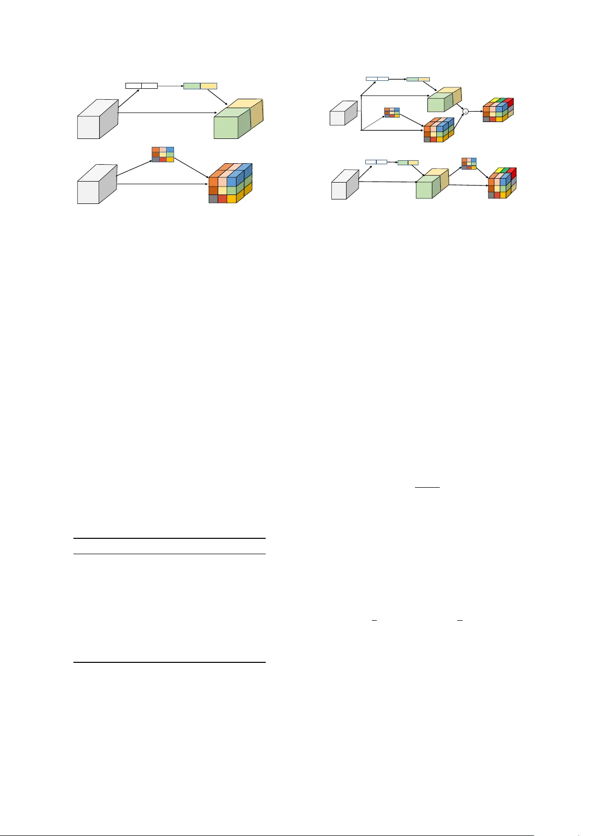
Sound Event Detection in Multichannel A udio using Con volutional T ime-Fr equency-Channel Squeeze and Excitation W ei Xia 1 , 2 , Kazuhito K oishida 2 1 Center for Robust Speech Systems, Uni versity of T e xas at Dallas, TX 75080 2 Microsoft Corporation, One Microsoft W ay , Redmond, W A 98052 wei.xia@utdallas.edu, kazukoi@microsoft.com Abstract In this study , we introduce a con volutional time-frequency- channel ”Squeeze and Excitation” (tfc-SE) module to explic- itly model inter-dependencies between the time-frequenc y do- main and multiple channels. The tfc-SE module consists of two parts: tf-SE block and c-SE block which are designed to provide attention on time-frequency and channel domain, re- spectiv ely , for adaptiv ely recalibrating the input feature map. The proposed tfc-SE module, together with a popular Conv o- lutional Recurrent Neural Network (CRNN) model, are ev alu- ated on a multi-channel sound event detection task with over - lapping audio sources: the training and test data are synthesized TUT Sound Ev ents 2018 datasets, recorded with microphone arrays. W e show that the tfc-SE module can be incorporated into the CRNN model at a small additional computational cost and bring significant improvements on sound event detection accuracy . W e also perform detailed ablation studies by analyz- ing v arious factors that may influence the performance of the SE blocks. W e sho w that with the best tfc-SE block, error rate (ER) decreases from 0.2538 to 0.2026, relativ e 20.17% reduction of ER, and 5.72% improvement of F1 score. The results indicate that the learned acoustic embeddings with the tfc-SE module efficiently strengthen time-frequency and channel-wise feature representations to improv e the discriminativ e performance. Index T erms : Sound event detection, squeece and excitation, attention, multichannel audio, conv olutional recurrent neural network 1. Introduction Sound event detection (SED) task in volves labeling the time stamps of a sound event in audio streams and detecting the sound type. Speech and non-speech sounds such as laughter and music contains lots of useful information. Being able to detect environmental sound e vents in multi-channel audios can greatly help us understand surrounding acoustic en vironments and enables many applications such as audio surveillance and rare sound detection [1, 2, 3]. It is also helpful to improve the performance of speech enhancement and separation systems if we could kno w the types of sounds [4, 5]. Robotic systems can employ SED for navigation and natural interaction with sur - rounding acoustic en vironments [6, 7]. Smart home devices can benefit from it for environmental sound understanding [8, 9]. Sound event detection is attracting more and more attention now adays from these applications, as well as multimedia con- tent retriev al [10, 11] and audio segmentation [12, 13, 14]. Real life audio recordings typically hav e many overlap- ping sound events, the task of recognizing all the overlapping sounds is considered as polyphonic SED. Lots of efforts hav e This work is done under Microsoft Research Internship program. been proposed to address this task by predicting frame-wise la- bels of each sound event class. Models like Gaussian Mixture Model (GMM) [15], Hidden Markov Model (HMM) [16], Re- current Neural Networks (RNN) [17, 18], and Conv olutional Neural Networks (CNN) [19, 20] have been explored exten- siv ely for this task. More recently successful results were ob- tained by stacking CNN, RNN and FC layers consecutiv ely , referred jointly as the con volutional recurrent neural network (CRNN) [21]. In order to improv e the recognition of overlap- ping sound events, several multi-channel SED methods hav e also been proposed. For example, Sharath [22, 23, 24] showed that Deep Neural Network can directly learn from low-le vel features such as generalized cross-correlation with phase based weighting (GCC-PHA T) for multi-channel sound detection. The basic building block for most SED models is the con- volutional layer , which learns filters capturing local spatial pat- terns along all the input channels and generates feature maps jointly encoding the time-frequency and channel information. A lot of work has aimed at impro ving the joint encoding of spa- tial and channel information [25], but much less attention has been gi ven to wards encoding of time-frequency and channel- wise patterns independently with domain information. Some re- cent work attempted to address this issue by explicitly modeling the inter -dependencies between the channels of feature maps. One promising approach to accomplish this is a component called ”Squeeze & Excitation” (SE) block [26, 27], which can be seamlessly integrated into the CNN model. This SE block factors out the spatial dependency by global average pooling to learn a channel specific descriptor , which is used to rescale the input feature map to highlight only useful channels. In this study , we introduce a time-frequency-channel Squeeze and Excitation (tfc-SE) block for multi-channel sound ev ent detection. Different from the original SE block men- tioned above, which uses global average pooling and only ex- cites on the channel axis, we adapt and extend it to both the time-frequency and channel domains. Multi-channel audio con- tains dif ferent information at each time-frequency location, for example, we may pay more attention to high energy parts in the spectrogram. W e first introduce a time-frequency SE (tf- SE) block that aims to adaptively recalibrate the learned fea- ture map. It does not change the recepti ve field, but provides time-frequency attention to certain regions. Further , we pro- pose two methods to combine the channel wise SE and time- frequency SE. These methods aggregate the unique properties of each block and make feature maps to be more informati ve on both domains. W e sho w that with the best tfc-SE block, er- ror rate of the SED system decreases from 0.2538 to 0.2026, relativ e 20.17% reduction of ER. It also has 5.72% relativ e im- prov ement of F1 score compared to the original CRNN. In the following sections, we describe the tfc-SE approach and corresponding baseline systems in Section 2. W e provide (a)$Channel$SE (b)$Time 0 Frequency$SE T T F F C C U U ! "# ! $% 1×1×C 1×1×C ! $&'(" T F C T F C ) ( * ) ! $&'(" s S T 1 × 1$conv F , - , - Figure 1: Channel SE and T ime-F r equency SE blocks. detailed explanations of our experiments in Section 3, as well as results and discussions in Section 4. Finally we conclude our work in Section 5. 2. Sound Event Detection Systems 2.1. Baseline Con volutional RNN W e use a recently proposed Con volutional Recurrent Neural Network (CRNN) [21] to learn the acoustic representations of multi-channel audio signals for sound ev ent detection. The CRNN model has three components, the con volutional layers to learn the time-frequency representations of audio waveform, the recurrent layers to learn the temporal information, and the final classification layer for sound ev ent detection. The model configuration is given in T able 1. W e use three layers of 2D CNN to learn the shift inv ariant features from multi-channel spectorgrams. Each CNN layer has P filters of a 3 × 3 ker - nel. After each CNN layer , we use a ReLU acti vation function and batch normalization to normalize the activ ations. A Max- pooling layer is applied on the frequenc y axis and the sequence length of T -frame input features are kept unchanged. T able 1: Baseline CRNN model ar chitectur e, when input are T = 256 frames, 256 dimensional and 16 c hannels features, P = 64 filters, Q = 128 nodes, R = 128 nodes, and N = 11 sound types. T ype Filter shape Input shape Con v1 3 × 3 × 16 × 64 256 × 256 × 16 Maxpool1 1 × 8 256 × 256 × 64 Con vol2 3 × 3 × 16 × 64 256 × 32 × 64 Maxpool2 1 × 8 256 × 4 × 64 Con vol3 3 × 3 × 16 × 64 256 × 4 × 64 Maxpool3 1 × 2 256 × 2 × 64 Bi-GR U1 - 256 × 128 Bi-GR U2 - 256 × 128 FC1 128 × 128 256 × 128 FC2 128 × 11 256 × 128 The output activ ation from CNN is further fed to bidirec- tional RNN layers which are designed to learn the temporal con- text information from the CNN output acti vations. Specifically , Q nodes of Gated Recurrent Units (GR U) are used in each layer with tanh acti vations. For classification, we use two fully con- nected (FC) layers. The first FC layer has R nodes each with (a)$Concurrent$time / fr equency / channel$SE (b)$Sequential$ time / frequency / channel$ SE ! U C C U F F T T T F C T F C element / wise operation Figure 2: Concurrent time-frequency-c hannel SE and sequen- tial time-fr equency-channel SE blocks. linear activ ation. The last FC layer consists of N nodes with sigmoid activ ations, each corresponding to one of the N sound ev ent classes to be detected. In the following sections, we introduce the ”Squeeze & Ex- citation” (SE) blocks. W e insert the SE block after each con- volutional layer to adapti vely recalibrate the feature representa- tions. 2.2. Channel wise squeeze and excitation 2.2.1. Squeeze operation The channel-wise SE block, c-SE, is illustrated in Fig. 1 (a). In order to model the inter-dependencies between multiple chan- nels of audio signals, we firstly define a squeeze operation to embed the global time-frequenc y information into a channel de- scriptor . W e consider the input feature map of the multi-channel audio as U = [ U 1 , U 2 , ..., U c ] where U c ∈ R T × F is the fea- ture matrix of channel c . W e use a global av erage pooling layer to generate a channel-wise vector z ∈ R 1 × 1 × C with its c -th element, z c = F sq ( U c ) = 1 T × F Σ T i Σ F j U c ( i, j ) (1) This operation embeds the global time-frequency information into the vector z . This vector contains statistics that are expres- siv e of the whole time-frequency input. 2.2.2. Excitation operation In order to capture channel wise dependencies, a gating mecha- nism with a sigmoid acti vation function is used to learn a non- linear relationship between channels, s = F ex ( z , W ) = σ ( g ( z , W )) = σ ( W 2 δ ( W 1 z )) (2) where W 1 ∈ R C r × C and W 2 ∈ R C × C r are weights of two fully-connected layers and δ is the ReLU operator . The dimen- sional reduction factor r indicates the bottleneck in the channel excitation block. Note that the original channel dimension is recov ered by the second FC layer . With a sigmoid layer σ , the channel-wise attention vector s is obtained. Finally we recali- brate U with the attention v ector as, ˆ X c = F scale ( U c , s c ) = s c · U c (3) ˆ X = [ ˆ X 1 , ˆ X 2 , ..., ˆ X C ] is the final channel wise recalibrated features. In this block, the input features are attentiv ely scaled so that important channels are emphasized and less important one are diminished. 2.3. Time-fr equency squeeze and excitation Here we introduce the time-frequency wise squeeze and e xcita- tion block (tf-SE), shown in Fig. 1 (b). The concept is similar to the c-SE and the main dif ference is to compress the feature map U along the channel axis using a 1-by-1 con volution [28]. The excitation operation is performed on the time-frequency map. W e assume that the time frequency space may contain more in- formation for SED. W e write the input feature map U in an alternate form, U =      u 1 , 1 u 1 , 2 ... u 1 ,F u 2 , 1 u 2 , 2 ... u 2 ,F . . . . . . . . . . . . u T , 1 u T , 2 ... u T ,F      (4) where u i,j ∈ R 1 × 1 × C is the feature bin at the time-frequency location ( i, j ) . The squeeze operation of the tf-SE is done using a 1-by-1 con volution which can be represented by the linear combination of all channels C at a location ( i, j ) , s i,j = σ (( w i,j ) T · u i,j ) (5) where w i,j is the filter coefficients and s i,j is the ( i, j ) -th el- ement of the squeezed matrix S ∈ R T × F . W e use a sigmoid function σ to limit the range of the matrix S to [0, 1], which is used to recalibrate the features on the time-frequency domain. Each value s i,j corresponds to the relativ e importance in the time-frequency space. Similar to the c-SE, the excitation of the tf-SE is carried out as ˆ x i,j = F scale ( u i,j , s i,j ) (6) and ˆ x i,j is the ( i, j ) -th element of the recalibrated output ˆ X . 2.4. Concurrent and sequential time-frequency-channel SE Each of the above explained c-SE and tf-SE blocks has its unique properties. The c-SE blocks recalibrates the channel in- formation by incorporating global time-frequency information. On the other hand, the tf-SE block generates an time-frequenc y attention map, indicating where the network should focus more to aid the sound classification. W e propose two ways to combine the complementary infor- mation from these two SE blocks to form the time-frequency- channel SE (tfc-SE): 1) Concurrent recalibration, illustrated in Fig. 2 (a) and 2) Sequential recalibration in order of channel first and then time-frequency as in Fig. 2 (b). For the concurrent tfc-SE, we present four ways to aggre- gate the c-SE and the tf-SE blocks. (i) Addition: the two recalibrated feature maps are added el- ement wise with equal weights. (ii) Multiplication: the feature maps are multiplied element wise. (iii) Maximization: each location ( i, j, c ) of the output feature map has the maximum activ ation of the two feature maps element-wise. (iv) Concatenation: the two feature maps are concatenated along the channel axis, which means that the volume of the input feature is twice larger . The concurrent tfc-SE and sequential tfc-SE with these aggre- gation strategies will be e valuated in the follo wing sections. 3. Experimental Setup 3.1. Dataset T o study the effecti veness of the CRNN model with the tfc- SE module in multi-channel sound ev ent detection, we used the synthetic eight-channel TUT Sound Events 2018 - Circular ar- ray , Rev erberant and Synthetic Impulse Response (CRESIM) dataset [23]. The dataset synthesizes the DCASE 2016 task 2 dataset [29], which has 11 isolated sound e vent classes such as speech, door slam, phone ringing, coughing, and keyboard. Each of the sound classes has 20 e xamples, of which 16 are randomly chosen for the training set and the rest 4 for the test set, in total 176 examples from 11 classes for training, and 44 for testing. W e selected the O3 subset which has maximum three temporally o verlapping sources. It consists of three cross- validation splits with 240 training and 60 testing recordings of length 30 sec sampled at 44100 Hz. In this dataset, circular microphone array recording is simulated with 8 omnidirectional microphones equally spaced on 5cm radius. More details can be found in [23]. 3.2. Featur e extraction On frame basis, we compute the magnitude and phase of spec- trograms and concatenate them along the channel axis as input features. A Hamming window of length M with 50% ov erlap is used to extract the spectrogram from each audio channel. The zeroth bin is e xcluded from the spectrogram, so that each frame produces a M / 2 × 16 feature matrix. The input feature is mean and variance normalized on the frame level. A sequence of the T -frame spectrograms are stacked and fed into the network. 3.3. Evaluation metrics W e ev aluated our sound detection model using the standard polyphonic SED metrics, error rate (ER) and F-score calculated on se gments of one second with no ov erlap as proposed in [30]. F1 (ideally F1 = 1) is based on true and false positi ves, and the error rate (ER) (ideally ER = 0) is based on the total number of activ e sound event classes in the ground truth. A joint SED error score can be considered as S S ED = ( E R + 1 − F ) / 2 . 3.4. Model configuration and training W e explored v arious CRNN models and feature configurations. It was found from preliminary experiments that the best input feature setting is a window length of M = 512 and sequence length of T = 256 (equiv alent to 1.486 sec). The CRNN model was trained on the CRESIM dataset for 1000 epochs with a batch size of 64. Early stopping was applied if there is no im- prov ement on the S S ED score after 100 epochs. W e built a various models with different parameters such as the number of nodes of CNN/RNN/FC and CNN filter size. The best base- line setting can be found in T able 1. The last fully connected layer has 11 nodes with sigmoid activation and the cross en- tropy loss for classification w as employed for netw ork training. W e used an Adam optimizer with the learning rate 10 − 3 . F or each sound e vent class all the predicted probabilities in the se- quence ( T = 256 ) were examined at the frame le vel and the class detection was claimed as true if there is any probability which is larger than a threshold of 0.5. 4. Results and Discussions 4.1. Experimental results In order to thoroughly evaluate our proposed methods, we will conduct detailed ablation analysis in this section. W e first per- form experiments on the c-SE, followed by the tf-SE, and then the sequential tfc-SE for sound ev ent detection. W e further in- vestigate the aggregation strategies for the concurrent tfc-SE. Finally we analyze various f actors that may affect the perfor- mance of SE blocks. From T able 2, we observe that our proposed channel wise SE (c-SE) block improves both F1 and ER compared with the original CRNN model. After utilizing the c-SE block, over - all error score S S ED of the model decreases from 0.2285 to 0.2194, relativ e 3.98% gain. This approach also achiev es rela- tiv e 6.30% improvement in ER. W e also find a consistent perfor- mance improvement with the time-frequency SE (tf-SE) block, relativ e 4.08% and 12.02% improvement in F1 and ER, respec- tiv ely , compared with the original CRNN model. The abov e results indicate that the tf-SE is more ef ficient than c-SE, which aligns with our assumption that the time-frequency space may hav e more meaningful information than channel for the SED task. Finally , we test the tfc-SE block which combines the c-SE and t-SE acti v ations. Both the concurrent and sequential mod- els improve the performance of the original CRNN model by a large margin. The best result is obtained with the sequential tfc-SE block, which achie ves 84.23% F1 score and 0.2026 error rate, relati ve 5.72% and 20.17% improvement compared with the original CRNN. In terms of the overall S S ED score, the se- quential tfc-SE block outperforms the original CRNN model by 21.18% relativ ely . T able 2: A verag ed SED results on CRESIM overlap 3 thr ee data splits using the CRNN model with time-fr equency-channel squeeze and excitation bloc ks. Model F1 (%) ER S S ED CRNN 79.67 0.2538 0.2285 +c-SE 79.91 0.2378 0.2194 +tf-SE 82.95 0.2233 0.1952 +tfc-SE concurrent 83.57 0.1982 0.1812 +tfc-SE sequential 84.23 0.2026 0.1801 4.2. Aggregation strategies W e further in vestigate the aggregation strategy of the concurrent tfc-SE block, among the four choices. W e observe from T able 3 that all aggregation methods increase the SED performance against the original CRNN. Using maximization pro vides the best performance. As concatenation aggregation increases the model comple xity by the doubled number of channels, maxi- mization operator looks a better choice for a lo wer computa- T able 3: SED r esults on CRESIM o verlap 3 split 1 subset us- ing CRNN + tfc-SE concurr ent block with differ ent aggr e gration operations. Aggregation F1(%) ER S S ED Addition 84.92 0.1791 0.1649 Multiplication 84.48 0.1959 0.1756 Maximization 85.79 0.1703 0.1562 Concatenation 85.26 0.1841 0.1657 tional cost. For all other experiments, we use the maximization- based aggregation for tfc-SE blocks. 4.3. Sensitivity to dimension r eduction ratio The reduction ratio r introduced in Section 2.2.2 is an important hyperparameter that allo ws us to vary the capacity and compu- tational cost of the c-SE blocks in the model. T able 4 reveals that the performance does not improve monotonically with in- creased capacity . This probably comes from ov erfitting due to a larger model capacity . W e find that r = 8 is a good option and we use it for our other experiments. T able 4: SED r esults on CRESIM o verlap 3 split 1 subset us- ing CRNN + tfc-SE concurrent block with differ ent dimension r eduction ratios. Ratio r F1(%) ER S S ED 2 85.07 0.1751 0.1622 4 85.59 0.1881 0.1661 8 85.79 0.1703 0.1562 16 83.51 0.1957 0.1803 4.4. Squeeze and excitation operator For the squeeze operator , we examine the significance of using global average pooling as opposed to global max pooling (while keeping the e xcitation operator sigmoid) in T able 5. Though both max and average pooling are effectiv e, average pooling achiev es a little better result and we use it all in our paper . W e next assess the excitation operator . T wo options, ReLU and tanh, are experimented by replacing from the sigmoid (with leaving the squeeze operator global average pooling). It sug- gests that it is important to choose the sigmoid operator in order to make the tfc-SE block ef fecti ve. T able 5: SED r esults on CRESIM o verlap 3 split 1 subset us- ing CRNN + tfc-SE concurr ent block with differ ent squeeze and excitation oper ators. Operator F1(%) ER S S ED Max 82.89 0.1971 0.1841 A vg 85.79 0.1703 0.1562 ReLU 83.42 0.1799 0.1728 T anh 82.58 0.2196 0.1969 Sigmoid 85.79 0.1703 0.1562 4.5. Model complexity The original CRNN model has 496,587 parameters. The tfc- SE block requires only 0.7% additional parameters, which is 500,067 in total. 5. Conclusions In this paper , we proposed a conv olutional time-frequency- channel squeeze and excitation block for multi-channel sound ev ent detection, in order to model the feature inter-dependencies between channels and the time-frequency locations. The tfc-SE block was inserted after each con volution layer of the CRNN model. The proposed method was e valuated on the CRESIM dataset and it was shown to improv e the original CRNN model in terms of both F1 score and error rate by a large margin. These results indicated that the tfc-SE block effecti vely recal- ibrates the feature maps adapti vely by emphasizing more im- portant channels and time-frequency locations. 6. References [1] J. Kotus, K. Lopatka, and A. Czyze wski, “Detection and localiza- tion of selected acoustic ev ents in acoustic field for smart surveil- lance applications, ” Multimedia T ools and Applications , vol. 68, no. 1, pp. 5–21, 2014. [2] P . Foggia, N. Petkov , A. Saggese, N. Strisciuglio, and M. V ento, “ Audio surveillance of roads: A system for detecting anomalous sounds, ” IEEE transactions on intelligent transportation systems , vol. 17, no. 1, pp. 279–288, 2016. [3] M. Crocco, M. Cristani, A. T rucco, and V . Murino, “ Audio surveillance: A systematic revie w , ” ACM Computing Surveys (CSUR) , vol. 48, no. 4, p. 52, 2016. [4] D. Stowell, D. Giannoulis, E. Benetos, M. Lagrange, and M. D. Plumbley , “Detection and classification of acoustic scenes and ev ents, ” IEEE T ransactions on Multimedia , vol. 17, no. 10, pp. 1733–1746, 2015. [5] Q. K ong, Y . Xu, W . W ang, and M. D. Plumbley , “ A joint separation-classification model for sound ev ent detection of weakly labelled data, ” in IEEE International Confer ence on Acoustics, Speech and Signal Pr ocessing (ICASSP) . IEEE, 2018, pp. 321–325. [6] R. T akeda and K. Komatani, “Sound source localization based on deep neural networks with directional acti vate function e xploiting phase information, ” in IEEE international conference on acous- tics, speech and signal pr ocessing (ICASSP) . IEEE, 2016, pp. 405–409. [7] W . He, P . Motlicek, and J.-M. Odobez, “Deep neural netw orks for multiple speaker detection and localization, ” in IEEE Interna- tional Conference on Robotics and A utomation (ICRA) . IEEE, 2018, pp. 74–79. [8] A. Southern, F . Stevens, and D. Murphy , “Sounding out smart cities: Auralization and soundscape monitoring for environmental sound design, ” The Journal of the Acoustical Society of America , vol. 141, no. 5, pp. 3880–3880, 2017. [9] C.-C. Kao, W . W ang, M. Sun, and C. W ang, “R-crnn: Region- based con volutional recurrent neural network for audio event de- tection, ” arXiv pr eprint arXiv:1808.06627 , 2018. [10] M. Xu, C. Xu, L. Duan, J. S. Jin, and S. Luo, “ Audio keywords generation for sports video analysis, ” ACM T ransactions on Mul- timedia Computing, Communications, and Applications (TOMM) , vol. 4, no. 2, p. 11, 2008. [11] Q. Jin, P . Schulam, S. Rawat, S. Burger , D. Ding, and F . Metze, “Event-based video retriev al using audio, ” in Thirteenth Annual Confer ence of the International Speech Communication Associa- tion , 2012. [12] A. Kumar and B. Raj, “ Audio event detection using weakly la- beled data, ” in Pr oceedings of the 24th A CM international confer- ence on Multimedia . ACM, 2016, pp. 1038–1047. [13] M. Tian, G. Fazekas, D. A. Black, and M. Sandler , “On the use of the tempogram to describe audio content and its application to music structural segmentation, ” in IEEE International Confer ence on Acoustics, Speech and Signal Processing (ICASSP) . IEEE, 2015, pp. 419–423. [14] G. Wichern, J. Xue, H. Thornburg, B. Mechtley , and A. Spanias, “Segmentation, inde xing, and retrie val for en vironmental and nat- ural sounds, ” IEEE Tr ansactions on Audio, Speech, and Language Pr ocessing , vol. 18, no. 3, pp. 688–707, 2010. [15] P . K. Atre y , N. C. Maddage, and M. S. Kankanhalli, “ Audio based ev ent detection for multimedia surv eillance, ” in IEEE Interna- tional Conference on Acoustics Speech and Signal Processing Pr oceedings (ICASSP) , vol. 5. IEEE, 2006. [16] A. Mesaros, T . Heittola, A. Eronen, and T . V irtanen, “ Acoustic ev ent detection in real life recordings, ” in Eur opean Signal Pro- cessing Confer ence . IEEE, 2010, pp. 1267–1271. [17] T . Hayashi, S. W atanabe, T . T oda, T . Hori, J. Le Roux, K. T akeda, T . Hayashi, S. W atanabe, T . T oda, T . Hori et al. , “Duration-controlled lstm for polyphonic sound ev ent detection, ” IEEE/ACM Tr ansactions on Audio, Speech and Languag e Pro- cessing (T ASLP) , vol. 25, no. 11, pp. 2059–2070, 2017. [18] G. Parascandolo, H. Huttunen, and T . V irtanen, “Recurrent neural networks for polyphonic sound e vent detection in real life record- ings, ” in IEEE International Conference on Acoustics, Speech and Signal Pr ocessing (ICASSP) . IEEE, 2016, pp. 6440–6444. [19] S. Hershey , S. Chaudhuri, D. P . Ellis, J. F . Gemmeke, A. Jansen, R. C. Moore, M. Plakal, D. Platt, R. A. Saurous, B. Se ybold et al. , “Cnn architectures for large-scale audio classification, ” in IEEE International Confer ence on Acoustics Speech and Signal Pr o- cessing (ICASSP) . IEEE, 2017, pp. 131–135. [20] H. Zhang, I. McLoughlin, and Y . Song, “Robust sound event recognition using conv olutional neural networks, ” in IEEE inter- national conference on acoustics, speech and signal processing (ICASSP) . IEEE, 2015, pp. 559–563. [21] E. Cakır , G. Parascandolo, T . Heittola, H. Huttunen, and T . V irtanen, “Conv olutional recurrent neural networks for poly- phonic sound event detection, ” IEEE/ACM T ransactions on Au- dio, Speech, and Language Processing , vol. 25, no. 6, pp. 1291– 1303, 2017. [22] S. Adav anne, P . Pertil ¨ a, and T . V irtanen, “Sound event detection using spatial features and con volutional recurrent neural network, ” in IEEE International Conference on Acoustics, Speech and Sig- nal Pr ocessing (ICASSP) . IEEE, 2017, pp. 771–775. [23] S. Adavanne, A. Politis, J. Nikunen, and T . V irtanen, “Sound ev ent localization and detection of ov erlapping sources using con- volutional recurrent neural networks, ” IEEE Journal of Selected T opics in Signal Processing , 2018. [24] S. Adav anne, A. Politis, and T . V irtanen, “Multichannel sound ev ent detection using 3d conv olutional neural networks for learn- ing inter-channel features, ” in 2018 International Joint Confer- ence on Neural Networks (IJCNN) . IEEE, 2018, pp. 1–7. [25] J. Dai, H. Qi, Y . Xiong, Y . Li, G. Zhang, H. Hu, and Y . W ei, “De- formable con volutional networks, ” in Pr oceedings of the IEEE in- ternational confer ence on computer vision , 2017, pp. 764–773. [26] J. Hu, L. Shen, and G. Sun, “Squeeze-and-excitation networks, ” in Proceedings of the IEEE conference on computer vision and pattern r ecognition , 2018, pp. 7132–7141. [27] A. G. Roy , N. Nav ab, and C. W achinger, “Concurrent spatial and channel squeeze & excitationin fully con volutional networks, ” in International Conference on Medical Imag e Computing and Computer-Assisted Intervention . Springer , 2018, pp. 421–429. [28] M. Lin, Q. Chen, and S. Y an, “Network in network, ” arXiv pr eprint arXiv:1312.4400 , 2013. [29] G. L. E. Benetos, M. Lagrnge, “sound event de- tection in synthetic audio, ” [Online]. A vailable: https://ar chive .or g/details/dcase2016 task2 train de v , 2016. [30] A. Mesaros, T . Heittola, and T . V irtanen, “Metrics for polyphonic sound ev ent detection, ” Applied Sciences , vol. 6, no. 6, p. 162, 2016.