An Elementary Introduction to Kalman Filtering

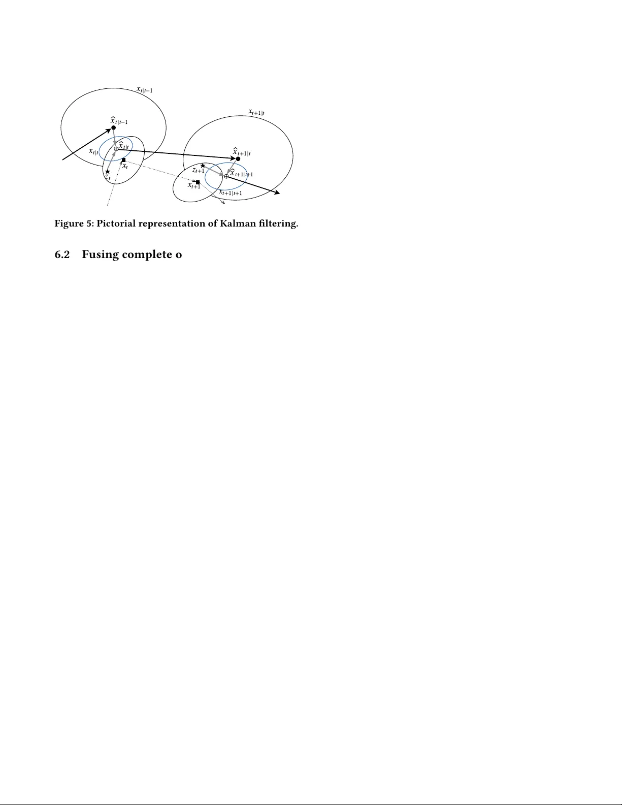
An Elementar y Introduction to K alman Filtering Y an Pei University of T exas at A ustin ypei@cs.utexas.edu Swarnendu Biswas Indian Institute of T echnology Kanpur swarnendu@cse.iitk.ac.in Donald S. Fussell University of T exas at A ustin fussell@cs.utexas.edu K eshav Pingali University of T exas at A ustin pingali@cs.utexas.edu ABSTRA CT Kalman ltering is a classic state estimation technique used in application areas such as signal processing and autonomous control of vehicles. It is now being used to solve problems in computer systems such as controlling the voltage and frequency of processors. Although there are many presentations of Kalman ltering in the literature, they usually deal with particular systems like autonomous robots or linear systems with Gaussian noise, which makes it dicult to understand the general principles behind K alman ltering. In this paper , we rst present the abstract ideas behind Kalman ltering at a level accessible to anyone with a basic knowledge of probability theory and calculus, and then show how these concepts can be applie d to the particular problem of state estimation in linear systems. This separation of concepts from applications should make it easier to understand Kalman ltering and to apply it to other problems in computer systems. KEY W ORDS Kalman ltering, data fusion, uncertainty , noise, state esti- mation, covariance, BLUE, linear systems 1 IN TRODUCTION Kalman ltering is a state estimation technique invented in 1960 by Rudolf E. Kálmán [ 16 ]. Be cause of its ability to extract useful information from noisy data and its small com- putational and memory requirements, it is used in many application areas including spacecraft navigation, motion planning in robotics, signal processing, and wireless sen- sor networks [ 12 , 21 , 28 – 30 ]. Recent work has used Kalman ltering in controllers for computer systems [ 5 , 13 , 14 , 24 ]. Although many introductions to Kalman ltering are avail- able in the literature [ 1 – 4 , 6 – 11 , 18 , 22 , 26 , 30 ], they are usu- ally focused on particular applications like robot motion or state estimation in linear systems. This can make it dicult to see how to apply Kalman ltering to other problems. Other presentations derive Kalman ltering as an application of Bayesian inference assuming that noise is Gaussian. This leads to the common misconception that Kalman ltering can be applied only if noise is Gaussian [ 15 ]. The goal of this pap er is to present the abstract concepts behind Kalman ltering in a way that is accessible to most computer scien- tists while clarifying the key assumptions, and then show how the problem of state estimation in linear systems can be solved as an application of these general concepts. Abstractly , Kalman ltering can be seen as a particular approach to combining approximations of an unknown value to produce a better approximation. Suppose we use two de- vices of dierent designs to measure the temp erature of a CP U core. Because devices are usually noisy , the measur e- ments are likely to dier from the actual temperature of the core. Since the devices are of dierent designs, let us assume that noise aects the two devices in unrelated ways (this is formalized using the notion of correlation in Section 2 ). Therefore, the measurements x 1 and x 2 are likely to be dif- ferent from each other and from the actual core temperature x c . A natural question is the following: is there a way to combine the information in the noisy measurements x 1 and x 2 to obtain a good approximation of the actual temperature x c ? One ad hoc solution is to use the formula 0 . 5 ∗ x 1 + 0 . 5 ∗ x 2 to take the average of the two measurements, giving them equal weight. Formulas of this sort are called linear estimators because they use a weighted sum to fuse values; for our temperature problem, their general form is β ∗ x 1 + α ∗ x 2 . In this paper , w e use the term estimate to refer to both a noisy measurement and to a value computed by an estimator , since both are approximations of unknown values of inter est. Suppose we have additional information ab out the two devices; say the se cond one uses more advanced tempera- ture sensing. Since we would have more condence in the second measurement, it se ems reasonable that we should discard the rst one, which is equivalent to using the linear estimator 0 . 0 ∗ x 1 + 1 . 0 ∗ x 2 . Kalman ltering tells us that in general, this intuitively reasonable linear estimator is not “optimal”; parado xically , ther e is useful information even in the measurement from the lower-quality device , and the op- timal estimator is one in which the weight given to each measurement is proportional to the condence w e have in the device producing that measurement. Only if we have no condence whatever in the rst de vice should we discard its measurement. Section 2 describ es how these intuitive ideas can be quan- tied. Estimates are modele d as random samples from distri- butions , and condence in estimates is quantie d in terms of the variances and covariances of these distributions. 1 Sec- tions 3 - 5 develop the two key ideas behind Kalman ltering. (1) How should estimates be fused optimally? Section 3 shows how to fuse scalar estimates such as temperatures optimally . It is also shown that the problem of fusing more than two estimates can be re- duced to the problem of fusing tw o estimates at a time without any loss in the quality of the nal estimate. Section 4 extends these results to estimates that are vec- tors , such as state vectors repr esenting the estimated position and velocity of a robot. (2) In some applications, estimates are vectors but only a part of the vector can be measured dir ectly . For e x- ample, the state of a spacecraft may b e represented by its position and velocity , but only its position may be obser vable. In such situations, how do we obtain a complete estimate from a partial estimate? Section 5 shows how the Best Linear Unbiased Esti- mator (BLUE) can be used for this. Intuitively , it is assumed that there is a linear relationship between the observable and hidden parts of the state vector , and this relationship is used to compute an estimate for the hidden part of the state, given an estimate for the observable part. Section 6 uses these ideas to solve the state estimation problems for linear systems, which is the usual context for presenting Kalman lters. Section 7 briey discusses exten- sions of Kalman ltering for nonlinear systems. 2 FORMALIZA TION OF ESTIMA TES This section makes precise the notions of estimates and con- dence in estimates. 2.1 Scalar estimates T o model the b ehavior of devices producing noisy measure- ments, we associate each device i with a random variable that has a probability density function (pdf ) p i ( x ) such as the ones shown in Figure 1 (the x-axis in this gure represents temperature). Random variables need not b e Gaussian. 2 Ob- taining a measurement from device i corresponds to drawing a random sample from the distribution for that device . W e write x i ∼ p i ( µ i , σ 2 i ) to denote that x i is a random variable 1 Basic concepts including probability density function, mean, expectation, variance and covariance are introduced in Appendix A . 2 The role of Gaussians in Kalman ltering is discussed in Section 6.5 . x 58 ◦ C 60 ◦ C 63 ◦ C p 1 ( x ) p 2 ( x ) p ( x ) Figure 1: Using pdfs to model devices with systematic and random errors. Ground truth is 60 ◦ C . Dashed lines are means of pdfs. with pdf p i whose mean and variance are µ i and σ 2 i respec- tively; following convention, we use x i to represent a random sample from this distribution as well. Means and variances of distributions model dierent kinds of inaccuracies in measurements. De vice i is said to have a systematic error or bias in its measurements if the mean µ i of its distribution is not equal to the actual temperature x c (in general, to the value b eing estimated, which is known as ground truth ); otherwise, the instrument is unbiased . Figure 1 shows pdfs for two devices that have dier ent amounts of systematic error . The variance σ 2 i on the other hand is a mea- sure of the random error in the measurements. The impact of random errors can be mitigate d by taking many measure- ments with a given device and averaging their values, but this approach will not help to reduce systematic error . In the usual formulation of K alman ltering, it is assumed that measuring devices do not have systematic errors. How- ever , we do not have the luxur y of taking many measure- ments of a given state, so we must take into account the impact of random error on a single measurement. Therefore , condence in a device is modeled formally by the variance of the distribution associated with that device; the smaller the variance , the higher our condence in the measurements made by the device . In Figure 1 , the fact that we have less condence in the rst device has b een illustrated by making p 1 more spread out than p 2 , giving it a larger variance. The informal notion that noise should aect the tw o de- vices in “unrelated ways” is formalized by requiring that the corresponding random variables be uncorrelated . This is a weaker condition than r equiring them to be independent , as explained in the Appendix A . Supp ose we ar e given the measurement made by one of the devices (say x 1 ) and we have to guess what the other measurement ( x 2 ) might be. If knowing x 1 does not give us any new information ab out what x 2 might be, the random variables are independent. This is expressed formally by the equation p ( x 2 | x 1 ) = p ( x 2 ) ; intuitively , knowing the value of x 1 does not change the pdf for the possible values of x 2 . If the random variables are 2 only uncorrelated, knowing x 1 might give us new informa- tion about x 2 such as restricting its possible values but the mean of x 2 | x 1 will still be µ 2 . Using expectations, this can be written as E [ x 2 | x 1 ] = E [ x 2 ] , which is equivalent to requiring that E [( x 1 − µ 1 )( x 2 − µ 2 )] , the covariance b etween the two vari- ables, be e qual to zero. This is obviously a weaker condition than independence. Although the discussion in this section has focused on measurements, the same formalization can be used for esti- mates produced by an estimator . Lemma 2.1 (i) shows how the mean and variance of a linear combination of pairwise uncorrelated random variables can be computed from the means and variances of the random variables [ 19 ]. The mean and variance can be used to quantify bias and random errors for the estimator as in the case of measurements. An unbiased estimator is one whose mean is equal to the unknown value being estimated and it is preferable to a bi- ased estimator with the same variance. Only unbiased estima- tors are considered in this paper . Furthermore, an unbiased estimator with a smaller variance is preferable to one with a larger variance since we would have more condence in the estimates it produces. As a step towards generalizing this discussion to estimators that pr oduce vector estimates, we refer to the variance of an unbiase d scalar estimator as the Mean Square Error of that estimator or MSE for short. Lemma 2.1 (ii) asserts that if a random variable is pair wise uncorrelated with a set of random variables, it is uncorrelated with any linear combination of those variables. Lemma 2.1. Let x 1 ∼ p 1 ( µ 1 , σ 2 1 ) , . . ., x n ∼ p n ( µ n , σ 2 n ) b e a set of pairwise uncorrelated random variables. Let y = Í n i = 1 α i x i be a random variable that is a linear combination of the x i ’s. (i) The mean and variance of y are: µ y = n Õ i = 1 α i µ i (1) σ 2 y = n Õ i = 1 α 2 i σ 2 i (2) (ii) If a random variable x n + 1 is pair wise uncorrelated with x 1 , . ., x n , it is uncorrelated with y . 2.2 V ector estimates In some applications, estimates are vectors. For example , the state of a mobile robot might be represented by a vector containing its position and velocity . Similarly , the vital signs of a person might be represented by a vector containing his temperature, pulse rate and blood pressure. In this paper , we denote a vector by a b oldfaced lowercase letter , and a matrix by an uppercase letter . The covariance matrix Σ xx of a random variable x is the matrix E [( x − µ µ µ x )( x − µ µ µ x ) T ] , where µ µ µ x is the mean of x . In- tuitively , entr y ( i , j ) of this matrix is the covariance between the i and j components of vector x ; in particular , entry ( i , i ) is the variance of the i t h component of x . A random variable x with a p df p whose mean is µ x µ x µ x and covariance matrix is Σ xx is written as x ∼ p ( µ x µ x µ x , Σ xx ) . The inverse of the covariance matrix ( Σ − 1 xx ) is called the precision or information matrix. Uncorrelated random variables : The cross-covariance ma- trix Σ vw of two random variables v and w is the matrix E [( v − µ µ µ v )( w − µ µ µ w ) T ] . Intuitively , element ( i , j ) of this matrix is the covariance between elements v ( i ) and w ( j ) . If the ran- dom variables are uncorrelated, all entries in this matrix are zero, which is equivalent to saying that every component of v is uncorrelated with every component of w . Lemma 2.2 generalizes Lemma 2.1 . Lemma 2.2. Let x 1 ∼ p 1 ( µ µ µ 1 , Σ 1 ) , . . ., x n ∼ p n ( µ µ µ n , Σ n ) be a set of pairwise uncorrelated random variables of length m . Let y = Í n i = 1 A i x i . (i) The mean and covariance matrix of y are the following: µ µ µ y = n Õ i = 1 A i µ µ µ i (3) Σ yy = n Õ i = 1 A i Σ i A T i (4) (ii) If a random variable x n + 1 is pair wise uncorrelated with x 1 , . ., x n , it is uncorrelated with y . The MSE of an unbiase d estimator y is E [( y − µ µ µ y ) T ( y − µ µ µ y )] , which is the sum of the variances of the comp onents of y ; if y has length 1, this reduces to variance as expe cted. The MSE is also the sum of the diagonal elements of Σ yy (this is called the trace of Σ yy ). 3 F USING SCALAR ESTIMA TES Section 3.1 discusses the problem of fusing two scalar esti- mates. Section 3.2 generalizes this to the problem of fusing n > 2 scalar estimates. Section 3.3 shows that fusing n > 2 esti- mates can be done iteratively by fusing two estimates at a time without any loss of quality in the nal estimate. 3.1 Fusing two scalar estimates W e now consider the problem of cho osing the optimal values of the parameters α and β in the linear estimator β ∗ x 1 + α ∗ x 2 for fusing estimates x 1 and x 2 from uncorrelated random variables. The rst reasonable requirement is that if the two esti- mates x 1 and x 2 are equal, fusing them should produce the same value. This implies that α + β = 1 . Therefore the linear 3 estimators of interest are of the form y α ( x 1 , x 2 ) = ( 1 − α )∗ x 1 + α ∗ x 2 (5) If x 1 and x 2 in Equation 5 are considered to be unbiased estimators of some quantity of interest, then y α is an unbi- ased estimator for any value of α . How should optimality of such an estimator be dened? One reasonable denition is that the optimal value of α minimizes the variance of y α since this will produce the highest-condence fused esti- mates as discussed in Se ction 2 . The variance ( MSE ) of y α can be determined from Lemma 2.1 : σ 2 y ( α ) = ( 1 − α ) 2 ∗ σ 2 1 + α 2 ∗ σ 2 2 (6) Theorem 3.1. Let x 1 ∼ p 1 ( µ 1 , σ 2 1 ) and x 2 ∼ p 2 ( µ 2 , σ 2 2 ) be un- correlated random variables. Consider the linear estimator y α ( x 1 , x 2 ) = ( 1 − α )∗ x 1 + α ∗ x 2 . The variance of the estimator is minimized for α = σ 2 1 σ 2 1 + σ 2 2 . This result can b e proved by setting the derivative of σ 2 y ( α ) with respect to α to zero and solving equation for α . Proof. d d α σ 2 y ( α ) = − 2 ( 1 − α ) ∗ σ 2 1 + 2 α ∗ σ 2 2 = 2 α ∗ ( σ 2 1 + σ 2 2 ) − 2 ∗ σ 2 1 = 0 α = σ 2 1 σ 2 1 + σ 2 2 (7) The second order derivative of σ 2 y ( α ) , ( σ 2 1 + σ 2 2 ) , is positive, showing that σ 2 y ( α ) reaches a minimum at this point. □ In the literature, the optimal value of α is called the Kalman gain K . Substituting K into the linear fusion model, we get the optimal linear estimator y ( x 1 , x 2 ) : y ( x 1 , x 2 ) = σ 2 2 σ 2 1 + σ 2 2 ∗ x 1 + σ 2 1 σ 2 1 + σ 2 2 ∗ x 2 (8) As a step to wards fusion of n > 2 estimates, it is useful to rewrite this as follows: y ( x 1 , x 2 ) = 1 σ 2 1 1 σ 2 1 + 1 σ 2 2 ∗ x 1 + 1 σ 2 2 1 σ 2 1 + 1 σ 2 2 ∗ x 2 (9) Substituting the optimal value of α into Equation 6 , we get σ 2 y = 1 1 σ 2 1 + 1 σ 2 2 (10) The expressions for y and σ 2 y are complicated be cause they contain the reciprocals of variances. If we let ν 1 and ν 2 denote the precisions of the two distributions, the expressions for y and ν y can be written more simply as follows: y ( x 1 , x 2 ) = ν 1 ν 1 + ν 2 ∗ x 1 + ν 2 ν 1 + ν 2 ∗ x 2 (11) ν y = ν 1 + ν 2 (12) These results say that the weight we should give to an estimate is proportional to the condence we have in that estimate, and that we hav e more condence in the fused es- timate than in the individual estimates, which is intuitively reasonable. T o use these results, we nee d only the variances of the distributions. In particular , the p dfs p i , which are usu- ally not available in applications, are not ne eded, and the proof of The orem 3.1 does not require these pdf ’s to have the same mean. 3.2 Fusing multiple scalar estimates The approach in Section 3.1 can b e generalized to optimally fuse multiple pairwise uncorrelated estimates x 1 , x 2 , . . ., x n . Let y n , α ( x 1 , . ., x n ) denote the linear estimator for fusing the n estimates given parameters α 1 , . ., α n , which we denote by α . The notation y α ( x 1 , x 2 ) introduced in the previous section can be considered to be an abbreviation of y 2 , α ( x 1 , x 2 ) . Theorem 3.2. Let x i ∼ p i ( µ i , σ 2 i ) for ( 1 ≤ i ≤ n ) b e a set of pairwise uncorrelated random variables. Consider the linear estimator y n , α ( x 1 , . ., x n ) = Í n i = 1 α i x i where Í n i = 1 α i = 1 . The variance of the estimator is minimized for α i = 1 σ 2 i Í n j = 1 1 σ 2 j Proof. From Lemma 2.1 , σ 2 y ( α ) = Í n i = 1 α i 2 σ i 2 . T o nd the values of α i that minimize the variance σ 2 y under the con- straint that the α i ’s sum to 1 , we use the method of Lagrange multipliers. Dene f ( α 1 , . . ., α n ) = n Õ i = 1 α i 2 σ i 2 + λ ( n Õ i = 1 α i − 1 ) where λ is the Lagrange multiplier . T aking the partial deriva- tives of f with respect to each α i and setting these derivatives to zero, we nd α 1 σ 2 1 = α 2 σ 2 2 = . . . = α n σ 2 n = − λ / 2 . From this, and the fact that sum of the α i ’s is 1 , the result follows. □ The minimal variance is given by the following expression: σ 2 y n = 1 n Õ j = 1 1 σ 2 j (13) As in Section 3.1 , these e xpressions are more intuitive if the variance is replaced with pr ecision: the contribution of x i 4 to the value of y n ( x 1 , . ., x n ) is proportional to x i ’s condence. y n ( x 1 , . ., x n ) = n Õ i = 1 ν i ν 1 + . . . + ν n ∗ x i (14) ν y n = n Õ i = 1 ν i (15) Equations 14 and 15 generalize Equations 11 and 12 . 3.3 Incremental fusing is optimal In many applications, the estimates x 1 , x 2 , . . ., x n become available successiv ely ov er a perio d of time. While it is possi- ble to store all the estimates and use Equations 14 and 15 to fuse all the estimates from scratch whenever a new estimate becomes available, it is possible to save b oth time and storage if one can do this fusion incrementally . W e show that just as a sequence of numbers can be added by keeping a running sum and adding the numbers to this running sum one at a time, a sequence of n > 2 estimates can be fused by ke eping a “running estimate” and fusing estimates from the sequence one at a time into this running estimate without any loss in the quality of the nal estimate. In short, w e want to show that y n ( x 1 , x 2 , . . ., x n ) = y 2 ( y 2 ( y 2 ( x 1 , x 2 ) , x 3 ) . . . , x n ) . A little bit of algebra shows that if n > 2 , Equations 14 and 15 for the optimal linear estimator and its pr ecision can be expressed as shown in Equations 16 and 17 . y n ( x 1 , . ., x n ) = ν y n − 1 ν y n − 1 + ν n y n − 1 ( x 1 , . . ., x n − 1 ) + ν n ν y n − 1 + ν n x n (16) ν y n = ν y n − 1 + ν n (17) This shows that y n ( x 1 , . ., x n ) = y 2 ( y n − 1 ( x 1 , . ., x n − 1 ) , x n ) . Using this argument recursively gives the requir ed result. 3 T o make the connection to Kalman ltering, it is useful to derive the same result using a pictorial argument. Fig- ure 2 shows the process of incrementally fusing the n es- timates. In this picture, time progresses from left to right, the precision of each estimate is shown in parentheses next to it, and the weights on the edges are the weights from Equation 11 . The contribution of each x i to the nal value y 2 ( y 2 ( y 2 ( x 1 , x 2 ) , x 3 ) . . . , x n ) is given by the product of the weights on the path from x i to the nal value and this product is ob- viously e qual to the weight of x i in Equation 14 , showing that incremental fusion is optimal. 3.4 Summary The results in this section can b e summarize d informally as follows. When using a linear estimator to fuse uncertain scalar estimates, the weight given to each estimate should be 3 W e thank Mani Chandy for sho wing us this approach to pr oving the r esult. + ( ν 1 ) x 1 ν 1 ν 1 + ν 2 x 2 ( ν 2 ) ν 2 ν 1 + ν 2 y ( x 1 , x 2 ) ( ν 1 + ν 2 ) + x 3 ( ν 3 ) ν 1 + ν 2 ν 1 + ν 2 + ν 3 ν 3 ν 1 + ν 2 + ν 3 . . . y 2 ( y 2 ( x 1 , x 2 ) , x 3 ) ( ν 1 + ν 2 + ν 3 ) + x n − 1 ( ν n − 1 ) ν n − 1 ν 1 + ·· · + ν n − 1 y 2 ( y 2 ( . . . ) , x n − 1 ) ( ν 1 + · · · + ν n − 1 ) + x n ( ν n ) ν n ν 1 + ·· · + ν n ν 1 + ·· · + ν n − 1 ν 1 + ·· · + ν n y 2 ( y 2 ( . . . ) , x n ) ( ν 1 + · · · + ν n ) Figure 2: Dataow graph for incremental fusion. inversely proportional to the variance of the random variable from which that estimate is obtained. Furthermore, when fus- ing n > 2 estimates, estimates can b e fused incrementally with- out any loss in the quality of the nal result. These results ar e often expressed formally in terms of the K alman gain K , as shown b elow; the e quations can be applied recursively to fuse multiple estimates. Note that if ν 1 ≫ ν 2 , K ≈ 0 and y ( x 1 , x 2 )≈ x 1 ; conversely if ν 1 ≪ ν 2 , K ≈ 1 and y ( x 1 , x 2 )≈ x 2 . x 1 ∼ p 1 ( µ 1 , σ 2 1 ) , x 2 ∼ p 2 ( µ 2 , σ 2 2 ) K = σ 2 1 σ 2 1 + σ 2 2 = ν 2 ν 1 + ν 2 (18) y ( x 1 , x 2 ) = x 1 + K ( x 2 − x 1 ) (19) σ 2 y = ( 1 − K ) σ 2 1 or ν y = ν 1 + ν 2 (20) 4 F USING VECTOR ESTIMA TES The results in Section 3 for fusing scalar estimates can b e extended to vectors by r eplacing variances with covariance matrices . 4.1 Fusing multiple vector estimates For vectors, the linear estimator is y n , A ( x 1 , x 2 , . ., x n ) = n Õ i = 1 A i x i where n Õ i = 1 A i = I (21) Here A stands for the matrix parameters ( A 1 , . . ., A n ) . All the vectors x i are assumed to be of the same length. T o simplify notation, we omit the subscript n in y n , A in the discussion below since it is obvious from the context. Optimality: The parameters A 1 , . . ., A n in the linear data fusion mo del are chosen to minimize MSE ( y A ) which is E [( y A − µ µ µ y A ) T ( y A − µ µ µ y A )] , as explained in Section 2 . Theorem 4.1 generalizes Theorem 3.2 to the vector case. The proof of this theorem uses matrix derivativ es [ 23 ] (see Appendix B ) and is given in Appendix C since it is not needed for understanding the rest of this pap er . Comparing The o- rems 4.1 and 3.2 , we see that the expressions are similar , the main dierence being that the role of variance in the scalar case is played by the covariance matrix in the vector case. 5 Theorem 4.1. Let x i ∼ p i ( µ i µ i µ i , Σ i ) for ( 1 ≤ i ≤ n ) b e a set of pairwise uncorrelated random variables. Consider the linear estimator y A ( x 1 , . ., x n ) = Í n i = 1 A i x i , where Í n i = 1 A i = I . The value of M S E ( y A ) is minimize d for A i = ( n Õ j = 1 Σ − 1 j ) − 1 Σ − 1 i (22) Therefore the optimal estimator is y ( x 1 , . . ., x n ) = ( n Õ j = 1 Σ − 1 j ) − 1 n Õ i = 1 Σ − 1 i x i (23) The covariance matrix of y can be computed by using Lemma 2.2 . Σ yy = ( n Õ j = 1 Σ − 1 j ) − 1 (24) In the vector case, precision is the inverse of a covariance matrix, denoted by N . Equations 25 – 26 use precision to ex- press the optimal estimator and its variance and generalize Equations 14 – 15 to the vector case. y ( x 1 , . . ., x n ) = N − 1 y n Õ i = 1 N i x i (25) N y = n Õ j = 1 N j (26) As in the scalar case, fusion of n > 2 vector estimates can be done incrementally without loss of precision. The proof is similar to the scalar case, and is omitted. There are se veral equivalent expressions for the K alman gain for the fusion of two estimates. The following one, which is easily derived from Equation 22 , is the vector analog of Equation 18 : K = Σ 1 ( Σ 1 + Σ 2 ) − 1 (27) The covariance matrix of the optimal estimator y ( x 1 , x 2 ) is the following. Σ yy = Σ 1 ( Σ 1 + Σ 2 ) − 1 Σ 2 (28) = K Σ 2 = Σ 1 − K Σ 1 (29) 4.2 Summary The r esults in this section can be summarized in terms of the Kalman gain K as follows. x 1 ∼ p 1 ( µ µ µ 1 , Σ 1 ) , x 2 ∼ p 2 ( µ µ µ 2 , Σ 2 ) K = Σ 1 ( Σ 1 + Σ 2 ) − 1 = ( N 1 + N 2 ) − 1 N 2 (30) y ( x 1 , x 2 ) = x 1 + K ( x 2 − x 1 ) (31) Σ yy = ( I − K ) Σ 1 or N y = N 1 + N 2 (32) 5 BEST LINEAR UNBIASED ESTIMA TOR (BLUE) In some applications, the state of the system is represented by a vector but only part of the state can be measured directly , so it is necessar y to estimate the hidden p ortion of the state corresponding to a measured value of the visible state. This section describ es an estimator calle d the Best Linear Unbiased Estimator (BLUE) [ 17 , 20 , 27 ] for doing this. x y x 1 b y 1  µ x µ y  ( b y − µ y ) = Σ yx Σ − 1 xx ( x − µ x ) Figure 3: BLUE line corresponding to Equation 33 . Consider the general problem of determining a value for vector y given a value for a vector x . If there is a functional relationship between x and y (say y = F ( x ) and F is given), it is easy to compute y given a value for x (say x 1 ). In our context howev er , x and y are random variables, so such a precise functional relationship will not hold. Figure 3 shows an example in which x and y are scalar-valued random variables. The gray ellipse in this gure , called a condence ellipse , is a projection of the joint distribution of x and y onto the ( x , y ) plane, that shows where some large pr oportion of the ( x , y ) values are likely to be. Supp ose x takes the value x 1 . Ev en within the condence ellipse, there are many points ( x 1 , y ) , so we cannot associate a single value of y with x 1 . One possibility is to compute the mean of the y values associated with x 1 (that is, the expectation E [ y | x = x 1 ] ), and return this as the estimate for y if x = x 1 . This requires knowing the joint distribution of x and y , which may not always be available. In some problems, we can assume that there is an un- known linear relationship between x and y and that uncer- tainty comes from noise. Therefor e, we can use a technique similar to the ordinary least squares (OLS) metho d to esti- mate this linear relationship, and use it to return the best estimate of y for any given value of x . In Figure 3 , w e see that although there are many points ( x 1 , y ) , the y values are clus- tered around the line shown in the gure so the value b y 1 is a reasonable estimate for the value of y corresponding to x 1 . This line, called the best linear unbiased estimator (BLUE), is the analog of ordinary least squares (OLS) for distributions. 6 Computing BLUE. Consider the estimator b y A , b ( x ) = A x + b . W e choose A and b so that this is an unbiased estimator with minimal MSE . The “ b ” over the y is notation that indicates that we are computing an estimate for y . Theorem 5.1. Let  x y  ∼ p (  µ µ µ x µ µ µ y  ,  Σ xx Σ xy Σ yx Σ yy  ) . The estima- tor b y A , b ( x ) = A x + b for estimating the value of y for a given value of x is an unbiased estimator with minimal MSE if b = µ µ µ y − A ( µ µ µ x ) A = Σ yx Σ − 1 xx The proof of Theorem 5.1 is straightforward. For an unbi- ased estimator , E [ b y ] = E [ y ] . This implies that b = µ µ µ y − A ( µ µ µ x ) so an unbiased estimator is of the form b y A ( x ) = µ µ µ y + A ( x − µ µ µ x ) . Note that this is equivalent to asserting that the BLUE line must pass through the point ( µ µ µ x , µ µ µ y ) . Setting the derivative of M S E A ( b y A ) with respect to A to zero[ 23 ] and solving for A , we nd that the best linear unbiased estimator is b y = µ µ µ y + Σ yx Σ − 1 xx ( x − µ µ µ x ) (33) This equation can be understo od intuitively as follows. If we hav e no information ab out x and y , the b est we can do is the estimate ( µ µ µ x , µ µ µ y ) , which lies on the BLUE line. However , if we know that x has a particular value x 1 , we can use the correlation between y and x to estimate a better value for y from the dierence ( x 1 − µ µ µ x ) . Note that if Σ yx = 0 (that is, x and y are uncorrelated), the best estimate of y is just µ µ µ y , so knowing the value of x does not give us any additional information about y as one would e xpect. In Figure 3 , this corresponds to the case when the BLUE line is parallel to the x-axis. At the other extreme, suppose that y and x are functionally related so y = C x . In that case, it is easy to see that Σ yx = C Σ xx , so b y = C x as expected. In Figure 3 , this corresponds to the case when the condence ellipse shrinks down to the BLUE line. Equation 33 is a generalization of ordinary least squares in the sense that if we compute the relevant means and variances of a set of discrete data ( x i , y i ) and substitute into Equation 33 , we get the same line that is obtained by using OLS. 6 KALMAN FILTERS FOR LINEAR SYSTEMS In this section, we apply the algorithms developed in Sec- tions 3 - 5 to the particular problem of state estimation in linear systems, which is the classical application of Kalman ltering. Figure 4a shows how the evolution of the state of such a system over time can be computed if the initial state x 0 and the model of the system dynamics are known precisely . Time advances in discrete steps. The state of the system at any time step is a function of the state of the system at the previous time step and the control inputs applied to the system during that interval. This is usually expressed by an equation of the form x t = f t ( x t − 1 , u t ) where u t is the control input. The function f t is nonlinear in the general case, and can be dierent for dierent steps. If the system is linear , the relation for state evolution over time can be written as x t = F t x t − 1 + B t u t , where F t and B t are time- dependent matrices that can be determined from the physics of the system. Therefore, if the initial state x 0 is known exactly and the system dynamics ar e modeled perfe ctly by the F t and B t matrices, the evolution of the state over time can be computed precisely as shown in Figure 4a . In general howev er , we may not know the initial state ex- actly , and the system dynamics and control inputs may not be known precisely . These inaccuracies may cause the state computed by the model to diverge unacceptably from the actual state over time. T o avoid this, we can make measure- ments of the state after each time step. If these measurements were e xact, there would of course be no need to model the system dynamics. However , in general, the measurements themselves are imprecise . Kalman ltering was invented to solve the problem of state estimation in such systems. Figure 4b shows the dataow of the computation, and we use it to introduce standard terminology . An estimate of the initial state, denote d by b x 0 | 0 , is assume d to be available. At each time step t = 1 , 2 , . . , the system model is used to provide an estimate of the state at time t using information from time t − 1 . This step is called prediction and the estimate that it provides is called the a priori estimate and denoted by b x t | t − 1 . The a priori estimate is then fused with z t , the state estimate obtained from the measurement at time t , and the result is the a posteriori state estimate at time t , denoted by b x t | t . This a posteriori estimate is used by the model to produce the a priori estimate for the next time step and so on. As describe d below , the a priori and a posteriori estimates are the means of certain random variables; the covariance matrices of these random variables are shown within parentheses above each estimate in Figure 4b , and these are used to weight estimates when fusing them. Section 6.1 presents the state evolution model and a priori state estimation. Section 6.2 discusses how state estimates are fused if an estimate of the entire state can b e obtained by measurement; Section 6.3 addresses this problem when only a portion of the state can be measured directly . 6.1 State evolution model and prediction The evolution of the state over time is described by a series of random variables x 0 , x 1 , x 2 ,... 7 x 0 x 1 x 2 f 1 f 2 ..... x t − 1 x t f t (a) Discrete-time dynamical system. + + b x 0 | 0 ( Σ 0 | 0 ) f 1 b x 1 | 0 ( Σ 1 | 0 ) b x 1 | 1 ( Σ 1 | 1 ) z 1 ( R 1 ) x 1 f 2 b x 2 | 1 ( Σ 2 | 1 ) z 2 ( R 2 ) x 2 b x 2 | 2 ( Σ 2 | 2 ) ..... + b x t − 1 | t − 1 ( Σ t − 1 | t − 1 ) f t b x t | t − 1 ( Σ t | t − 1 ) b x t | t ( Σ t | t ) z t ( R t ) x t (b) Dynamical system with uncertainty . ( Σ 0 | 0 ) b x 0 | 0 b x t | t − 1 = F t b x t − 1 | t − 1 + B t u t Σ t | t − 1 = F t Σ t − 1 | t − 1 F T t + Q t ( Σ t | t − 1 ) b x t | t − 1 K t = Σ t | t − 1 ( Σ t | t − 1 + R t ) − 1 b x t | t = b x t | t − 1 + K t ( z t - b x t | t − 1 ) Σ t | t = ( I - K t ) Σ t | t − 1 z t ( R t ) x t ( Σ t | t ) b x t | t Predictor Measurement Fusion + (c) Implementation of the dataow diagram ( b). ( Σ 0 | 0 ) b x 0 | 0 b x t | t − 1 = F t b x t − 1 | t − 1 + B t u t Σ t | t − 1 = F t Σ t − 1 | t − 1 F T t + Q t ( Σ t | t − 1 ) b x t | t − 1 K t = Σ t | t − 1 H t T ( H t Σ t | t − 1 H t T + R t ) − 1 b x t | t = b x t | t − 1 + K t ( z t - H t b x t | t − 1 ) Σ t | t = ( I - K t H t ) Σ t | t − 1 z t ( R t ) H t x t ( Σ t | t ) b x t | t Predictor Measurement Fusion + (d) Implementation of the dataow diagram ( b) for systems with partial observability . Figure 4: State estimation using Kalman ltering. • The random variable x 0 captures the likelihood of dif- ferent initial states. • The random variables at successive time steps are r e- lated by the following linear model: x t = F t x t − 1 + B t u t + w t (34) Here, u t is the control input, which is assumed to be deterministic, and w t is a zero-mean noise term that models all the uncertainty in the system. The covariance matrix of w t is denoted by Q t , and the noise terms in dierent time steps ar e assumed to be uncorrelated to each other (that is, E [ w i w j ] = 0 if i , j ) and to x 0 . For estimation, we hav e a random variable x 0 | 0 that cap- tures our b elief about the likelihood of dierent states at time t = 0 , and two random variables x t | t − 1 and x t | t at each time step t = 1 , 2 , . . . that capture our beliefs ab out the likeli- hood of dier ent states at time t before and after fusion with the measur ement r espectively . The mean and covariance ma- trix of a random variable x i | j are denoted by b x i | j and Σ i | j respectively . W e assume E [ b x 0 | 0 ] = E [ x 0 ] (no bias). Prediction essentially uses x t − 1 | t − 1 as a proxy for x t − 1 in Equation 34 to determine x t | t − 1 as shown in Equation 35 . x t | t − 1 = F t x t − 1 | t − 1 + B t u t + w t (35) For state estimation, we need only the mean and covari- ance matrix of x t | t − 1 . The Predictor box in Figure 4 com- putes these values; the co variance matrix is obtained from Lemma 2.2 under the assumption that w t is uncorrelated with x t − 1 | t − 1 , which is justied in Section 6.2 . 8 x ˆ t + 1 | t + 1 x t + 1 | t + 1 ⨁ x t + 1 z t + 1 x ˆ t + 1 | t x ˆ t | t ⨁ z t x t x ˆ t | t − 1 x t | t − 1 x t + 1 | t x t | t Figure 5: Pictorial representation of Kalman ltering. 6.2 Fusing complete obser vations of the state If the entire state can b e measured at each time step, the imprecise measurement at time t is mo deled as follows: z t = x t + v t (36) where v t is a zero-mean noise term with covariance matrix R t . The noise terms in dierent time steps are assumed to b e uncorrelated with each other (that is, E [ v i v j ] is zero if i , j ) as well as with x 0 | 0 and all w k . A subtle point here is that x t in this equation is the actual state of the system at time t (that is, a particular realization of the random variable x t ), so variability in z t comes only from v t and its covariance matrix R t . Therefore , we have two impr ecise estimates for the state at each time step t = 1 , 2 , . . . , the a priori estimate from the predictor ( b x t | t − 1 ) and the one from the measurement ( z t ). If z t is uncorrelated to x t | t − 1 , we can use Equations 30 - 32 to fuse the estimates as shown in Figure 4c . The assumptions that (i) x t − 1 | t − 1 is uncorrelated with w t , which is use d in prediction, and (ii) x t | t − 1 is uncorrelated with z t , which is use d in fusion, are easily prov ed to b e correct by induction on t , using Lemma 2.2 (ii). Figure 4b gives the intuition: x t | t − 1 for example is an ane function of the random variables x 0 | 0 , w 1 , v 1 , w 2 , v 2 , . . ., w t , and is therefore uncorrelated with v t (by assumption about v t and Lemma 2.2 (ii)) and hence with z t . Figure 5 shows the computation pictorially using con- dence ellipses to illustrate uncertainty . The dotted arrows at the bottom of the gure sho w the evolution of the state, and the solid arrows show the computation of the a priori estimates and their fusion with measurements. 6.3 Fusing partial obser vations of the state In some problems, only a portion of the state can b e mea- sured directly . The observable p ortion of the state is specie d formally using a full row-rank matrix H t called the observa- tion matrix : if the state is x , what is observable is H t x . For example, if the state vector has two components and only the rst component is obser vable, H t can b e [ 1 0 ] . In general, the H t matrix can specify a linear relationship between the state and the observation, and it can be time-dependent. The imprecise measurement model introduced in Equation 36 becomes: z t = H t x t + v t (37) The hidden portion of the state can b e specied using a matrix C t , which is an orthogonal complement of H t . For example, if H t = [ 1 0 ] , one choice for C t is [ 0 1 ] . Figure 4d shows the computation for this case. The fusion phase can b e understood intuitiv ely in terms of the follo wing steps. (i) The observable part of the a priori estimate of the state H t b x t | t − 1 is fused with the measurement z t , using the techniques developed in Sections 3 - 4 . The quantity z t − H t b x t | t − 1 is called the innovation . The result is the a p osteriori es- timate of the observable state H t b x t | t . (ii) The BLUE in Section 5 is used to obtain the a p os- teriori estimate of the hidden state C t b x t | t by adding to the a priori estimate of the hidden state C t b x t | t − 1 a value obtained from the product of the co variance be- tween H t x t | t − 1 and C t x t | t − 1 and the dierence between H t b x t | t − 1 and H t b x t | t . (iii) The a p osteriori estimates of the observable and hidden portions of the state are composed to produce the a posteriori estimate of the entire state b x t | t . The actual implementation produces the nal result di- rectly without going through these steps as shown in Fig- ure 4d , but these incremental steps are useful for understand- ing how all this w orks, and they are implemente d as follows. (i) The a priori estimate of the obser vable part of the state is H t b x t | t − 1 and the covariance is H t Σ t | t − 1 H T t . The a pos- teriori estimate is obtained directly from Equation 31 : H t b x t | t = H t b x t | t − 1 + H t Σ t | t − 1 H T t ( H t Σ t | t − 1 H T t + R t ) − 1 ( z t − H t b x t | t − 1 ) Let K t = Σ t | t − 1 H T t ( H t Σ t | t − 1 H T t + R t ) − 1 . The a posteriori estimate of the observable state can b e written in terms of K t as follows: H t b x t | t = H t b x t | t − 1 + H t K t ( z t − H t b x t | t − 1 ) (38) (ii) The a priori estimate of the hidden state is C t b x t | t − 1 . The covariance b etween the hidden portion C t x t | t − 1 and the obser vable portion H t x t | t − 1 is C t Σ t | t − 1 H T t . The dierence b etween the a priori estimate and a p osteriori estimate of H t x is H t K t ( z t − H b x t | t − 1 ) . Therefore the a posteriori estimate of the hidden portion of the state is 9 obtained directly from Equation 33 : C t b x t | t = C t b x t | t − 1 + ( C t Σ t | t − 1 H T t )( H t Σ t | t − 1 H T t ) − 1 H t K t ( z t − H t b x t | t − 1 ) = C t b x t | t − 1 + C t K t ( z t − H t b x t | t − 1 ) (39) (iii) Putting the a posteriori estimates ( 38 ) and ( 39 ) together ,  H t C t  b x t | t =  H t C t  b x t | t − 1 +  H t C t  K t ( z t − H t b x t | t − 1 ) Since  H t C t  is invertible, it can be canceled from the left and right hand sides, giving the equation b x t | t = b x t | t − 1 + K t ( z t − H t b x t | t − 1 ) (40) T o compute Σ t | t , Equation 40 can be rewritten as b x t | t = ( I − K t H t ) b x t | t − 1 + K t z t . Since x t | t − 1 and z t are un- correlated, it follows from Lemma 2.2 that Σ t | t = ( I − K t H t ) Σ t | t − 1 ( I − K t H t ) T + K t R t K T t Substituting the value of K t and simplifying, we get Σ t | t = ( I − K t H t ) Σ t | t − 1 (41) Figure 4d puts all this together . In the literature, this dataow is referred to as K alman ltering. Unlike in Se c- tions 3 and 4 , the Kalman gain is not a dimensionless value here. If H t = I , the computations in Figure 4d r educe to those of Figure 4c as expected. Equation 40 shows that the a posteriori state estimate is a linear combination of the a priori state estimate ( b x t | t − 1 ) and the measurement ( z t ). The optimality of this linear unbiased estimator is shown in the Appendix D . In Se ction 3.3 , it was shown that incremental fusion of scalar estimates is optimal. The dataow of Figures 4 (c,d) computes the a posteriori state estimate at time t by incrementally fusing measurements from the previous time steps, and this incremental fusion can be shown to be optimal using a similar argument. 6.4 Example: falling b o dy T o demonstrate the eectiveness of the Kalman lter, we consider an example in which an object falls from the origin at time t = 0 with an initial sp eed of 0 m/s and an expe cted constant acceleration of 9 . 8 m/s 2 due to gravity . Note that acceleration in reality may not be constant due to factors such as wind, air friction, and so on. The state vector of the object contains tw o components, one for the distance from the origin s ( t ) and one for the velocity v ( t ) . W e assume that only the velocity state can be measured at each time step. If time is discretized in steps of 0.25 seconds, the dierence equation for the dynamics of the system is easily shown to be the following:  v n s n  =  1 0 0 . 25 1   v n − 1 s n − 1  +  0 0 . 25 0 0 . 5 × 0 . 25 2   0 9 . 8  (42) where we assume  v 0 s 0  =  0 0  and Σ 0 =  80 0 0 10  . The gray lines in Figure 6 show the e volution of velocity and distance with time according to this model. Because of uncertainty in modeling the system dynamics, the actual evolution of the velocity and position will be dierent in practice. The red lines in Figure 6 show one trajector y for this evolution, corresponding to a Gaussian noise term with covariance  2 2 . 5 2 . 5 4  in Equation 34 (b ecause this noise term is random, there are many trajectories for the evolu- tion, and we are just showing one of them). The red lines correspond to “ground truth” in our example . The green p oints in Figure 6b show the noisy measure- ments of velocity at dierent time steps, assuming the noise is modele d by a Gaussian with variance 8 . The blue lines show the a posteriori estimates of the velocity and position. It can be se en that the a posteriori estimates track the ground truth quite well even when the ideal system model (the gray lines) is inaccurate and the measurements are noisy . The cyan bars in the right gure show the variance of the veloc- ity at dierent time steps. Although the initial variance is quite large, application of Kalman ltering is able to r educe it rapidly in few time steps. 6.5 Discussion This section shows that Kalman ltering for state estimation in linear systems can be derived from two elementar y ideas: optimal linear estimators for fusing uncorrelated estimates and best linear unbiased estimators for correlated variables. This is a dierent approach to the subject than the standard presentations in the literature. One standar d approach is to use Bayesian inference. The other approach is to assume that the a p osteriori state estimator is a linear combination of the form A t b x t | t − 1 + B t z t , and then nd the values of A t and B t that produce an unbiase d estimator with minimum MSE . W e believe that the advantage of the presentation given here is that it exposes the concepts and assumptions that underlie Kalman ltering. Most presentations in the literature also b egin by assuming that the noise terms w t in the state evolution e quation and v t in the measurement are Gaussian. Some presentations [ 1 , 10 ] use properties of Gaussians to derive the results in Se ctions 3 although as we have seen, these results do not dep end on distributions being Gaussians. Gaussians however enter the picture in a deeper way if one considers nonlinear estimators. It can be shown that if the noise terms are not Gaussian, there may be nonlinear estimators whose MSE is lower than that 10 0 5 10 15 20 Time (s) 0 500 1000 1500 2000 2500 Distance (m) Model-only Ground Truth Estimated (a) Evolution of state: Distance 0 5 10 15 20 Time (s) 0 50 100 150 200 250 300 Velocity (m/s) 0 25 50 75 100 125 150 Variance Model-only Ground Truth Estimated Measured Variance (b) Evolution of state: V elocity Figure 6: Estimates of the obje ct’s state over time. of the linear estimator presented in Figure 4d . However if the noise is Gaussian, this linear estimator is as go od as any unbiased nonlinear estimator (that is, the linear estimator is a minimum variance unbiase d estimator (MVUE)). This result is proved using the Cramer-Rao low er bound [ 25 ]. 7 EXTENSION TO NONLINEAR SYSTEMS The Extended Kalman Filter (EKF) and Unscented Kalman Fil- ter (UKF) are heuristic approaches to using Kalman ltering for nonlinear systems. The state evolution and measurement equations for nonlinear systems with additive noise can be written as follows; in these equations, f and h are nonlinear functions. x t = f ( x t − 1 , u t ) + w t (43) z t = h ( x t ) + v t (44) Intuitively , the EKF constructs linear approximations to the nonlinear functions f and h and applies the Kalman lter equations, while the UKF constructs approximations to probability distributions and propagates these through the nonlinear functions to construct approximations to the posterior distributions. EKF. Examining Figure 4d , we se e that the a priori state estimate in the predictor can be compute d using the system model: b x t | t − 1 = f ( b x t − 1 | t − 1 , u t ) . Howev er , since the system dynamics and measurement e quations are nonlinear , it is not clear how to compute the co variance matrices for the a priori estimate and the measurement. In the EKF, these matrices are computed by linearizing Equations 43 and 44 using the T aylor series expansions for the nonlinear functions f and h . This requires computing the following Jacobians 4 , which play the role of F t and H t in Figure 4d . F t = ∂ f ∂ x     b x t − 1 | t − 1 , u t H t = ∂ h ∂ x     b x t | t − 1 The EKF performs well in some applications such as navi- gation systems and GPS [ 29 ]. UKF. When the system dynamics and obser vation models are highly nonlinear , the Unscente d Kalman Filter ( UKF) [ 15 ] can be an improvement o ver the EKF . The UKF is based on the unscented transformation , which is a metho d for comput- ing the statistics of a random variable x that undergoes a nonlinear transformation ( y = д ( x ) ). The random variable x is sampled using a carefully chosen set of sigma p oints and these sample points are pr opagated through the nonlinear function д . The statistics of y are estimated using a weighted sample mean and covariance of the posterior sigma points. The UKF tends to b e more robust and accurate than the EKF but has higher computation overhead due to the sampling process. 8 CONCLUSION In this paper , we have shown that two concepts - optimal linear estimators for fusing uncorrelated estimates and best linear unbiased estimators for correlated variables - provide the underpinnings for Kalman ltering. By combining these ideas, standar d results on Kalman ltering for linear systems can be derived in an intuitive and straightforward way that is simpler than other presentations of this material in the 4 The Jacobian matrix is the matrix of all rst order partial derivatives of a vector-valued function. 11 literature. This appr oach makes clear the assumptions that underlie the optimality r esults associated with Kalman lter- ing, and should make it easier to apply K alman ltering to problems in computer systems. A CKNO WLEDGMEN TS This research was supp orted by NSF grants 1337281, 1406355, and 1618425, and by D ARP A contracts F A8750-16-2-0004 and F A8650-15-C-7563. The authors would like to thank K. Mani Chandy (Caltech), Ivo Babuska (U T A ustin) and A ugusto Ferrante (Padova) for their feedback on this paper . REFERENCES [1] Tim Babb. 2018. How a Kalman lter works, in pictures | Bzarg. https: //www.bzarg.com/p/ho w- a- kalman- lter- works- in- pictures/ . (2018). Accessed: 2018-11-30. [2] A. V . Balakrishnan. 1987. Kalman Filtering Theory . Optimization Software, Inc., Los Angeles, CA, USA. [3] Allen L. Barker , Donald E. Brown, and W orthy N. Martin. 1994. Bayesian Estimation and the Kalman Filter . T echnical Report. Char- lottesville, V A, USA. [4] Alex Becker . 2018. Kalman Filter Overview . https://ww w .kalmanlter . net/default.aspx . (2018). Accessed: 2018-11-08. [5] K. Bergman. 2009. Nanophotonic Interconnection Networks in Multi- core Embe dded Computing. In 2009 IEEE/LEOS Winter T opicals Meeting Series . 6–7. https://doi.org/10.1109/LEOSWT .2009.4771628 [6] Liyu Cao and Howard M. Schwartz. 2004. Analysis of the Kalman Filter Base d Estimation Algorithm: An Orthogonal De composition Approach. A utomatica 40, 1 (Jan. 2004), 5–19. https://doi.org/10.1016/ j.automatica.2003.07.011 [7] Charles K. Chui and Guanrong Chen. 2017. Kalman Filtering: With Real- Time A pplications (5th e d.). Springer Publishing Company , Incor- porated. [8] R.L. Eubank. 2005. A Kalman Filter Primer (Statistics: Te xtbooks and Monographs) . Chapman & Hall/CRC. [9] Geir Evensen. 2006. Data Assimilation: The Ensemble Kalman Filter . Springer- V erlag New Y ork, Inc., Secaucus, NJ, USA. [10] Rodney Faragher . 2012. Understanding the Basis of the Kalman Filter Via a Simple and Intuitive Derivation. IEEE Signal Processing Magazine 29, 5 (September 2012), 128–132. [11] Mohinder S. Grewal and Angus P. Andr ews. 2014. Kalman Filtering: Theory and Practice with MA TLAB (4th ed.). Wiley-IEEE Press. [12] Anne-Kathrin Hess and Anders Rantzer. 2010. Distributed Kalman Filter Algorithms for Self-localization of Mobile Devices. In Proce edings of the 13th A CM International Conference on Hybrid Systems: Compu- tation and Control (HSCC ’10) . ACM, New Y ork, N Y , USA, 191–200. https://doi.org/10.1145/1755952.1755980 [13] Connor Imes and Henry Homann. 2016. Bard: A Unied Framework for Managing Soft Timing and Power Constraints. In International Conference on Emb e dded Computer Systems: A rchitectures, Modeling and Simulation (SAMOS) . [14] C. Imes, D. H. K. Kim, M. Maggio, and H. Homann. 2015. POET: A Portable Approach to Minimizing Energy Under Soft Real-time Constraints. In 21 st IEEE Real-Time and Embedded T echnology and A pplications Symp osium . 75–86. https://doi.org/10.1109/RTAS.2015. 7108419 [15] Simon J. Julier and Jerey K. Uhlmann. 2004. Unscented Filtering and Nonlinear Estimation. Proc. IEEE 92, 3 (2004), 401–422. https: //doi.org/10.1109/JPROC.2003.823141 [16] Rudolph Emil Kalman. 1960. A New Approach to Linear Filtering and Prediction Problems. Transactions of the ASME–Journal of Basic Engineering 82, Series D (1960), 35–45. [17] Peter K Kitanidis. 1987. Unbiased Minimum-variance Linear State Estimation. A utomatica 23, 6 (Nov . 1987), 775–778. https://doi.org/10. 1016/0005- 1098(87)90037- 9 [18] Anders Lindquist and Giogio Picci. 2017. Linear Stochastic Systems . Springer- V erlag. [19] Peter S Mayb eck. 1982. Stochastic models, estimation, and control . V ol. 3. Academic press. [20] Jerry M Mendel. 1995. Lessons in Estimation Theor y for Signal Processing, Communications, and Control . Pearson Education. [21] Kaushik Nagarajan, Nicholas Gans, and Roozb eh Jafari. 2011. Mod- eling Human Gait Using a Kalman Filter to Measure W alking Dis- tance. In Proce edings of the 2nd Conference on Wireless Health (WH ’11) . A CM, New Y ork, NY, USA, Article 34, 2 pages. https://doi.org/10.1145/ 2077546.2077584 [22] Eduardo F. Nakamura, Antonio A. F . Loureiro, and Alejandro C. Frery . 2007. Information Fusion for Wireless Sensor Networks: Methods, Models, and Classications. A CM Comput. Surv . 39, 3, Article 9 (Sept. 2007). https://doi.org/10.1145/1267070.1267073 [23] Kaare Brandt Petersen and Michael Syskind Pe dersen. 2012. The Matrix Cookbook. http://www2.imm.dtu.dk/pub db/views/publication_details. php?id=3274 . (Nov . 2012). V ersion 20121115. [24] Raghavendra Pradyumna Pothukuchi, Amin Ansari, Petros V oulgaris, and Josep T orrellas. 2016. Using Multiple Input, Multiple Output Formal Control to Maximize Resource Eciency in Architectures. In Computer Ar chitecture (ISCA), 2016 ACM/IEEE 43rd Annual Interna- tional Symposium on . IEEE, 658–670. [25] C.R. Rao. 1945. Information and the Accuracy Attainable in the Esti- mation of Statistical Parameters. Bulletin of the Calcutta Mathematical Society 37 (1945), 81–89. [26] Matthew B. Rhudy , Roger A. Salguero, and K eaton Holappa. 2017. A Kalman Filtering T utorial for Undergraduate Students. International Journal of Computer Science & Engineering Sur vey 8, 1 (Feb. 2017). [27] Sailes K. Sengupta. 1995. Fundamentals of Statistical Signal Processing: Estimation Theory. T echnometrics 37, 4 (1995), 465–466. https://doi. org/10.1080/00401706.1995.10484391 [28] Éfren L. Souza, Eduardo F. Nakamura, and Richard W . Pazzi. 2016. T arget Tracking for Sensor Networks: A Survey. A CM Comput. Surv . 49, 2, Article 30 (June 2016), 31 pages. https://doi.org/10.1145/2938639 [29] Sebastian Thrun, W olfram Burgard, and Dieter Fox. 2005. Probabilistic Robotics (Intelligent Robotics and Autonomous Agents) . The MI T Press. [30] Greg W elch and Gar y Bishop. 1995. An Introduction to the Kalman Filter . Technical Report. Chapel Hill, NC, USA. [31] Y an Pei, Swarnendu Biswas, Donald S. Fussell, and Keshav Pingali. 2017. An Elementary Introduction to Kalman Filtering. A rXiv e-prints (Oct. 2017). arXiv: 1710.04055 12 Appendices A BASIC PROBABILI T Y THEORY AND ST A TISTICS TERMINOLOGY Probability density function. For a continuous random vari- able x , a probability density function (pdf ) is a function p ( x ) whose value provides a relativ e likelihood that the value of the random variable will equal x . The integral of the pdf within a range of values is the probability that the random variable will take a value within that range. If д ( x ) is a function of x with pdf p ( x ) , the expected value or expectation of д ( x ) is E [ д ( x )] , dened as the following integral: E [ д ( x )] = ∫ ∞ −∞ д ( x ) p ( x ) d x By denition, the mean µ x of a random variable x is E [ x ] . The variance of a random variable x measur es the variability of the distribution. For the set of possible values of x , variance (denoted by σ 2 x ) is dened by σ 2 x = E [( x − µ x ) 2 ] . The variance of a continuous random variable x can be written as the following integral: σ 2 x = ∫ ∞ −∞ ( x − µ ) 2 p ( x ) d x If x is discrete and all outcomes are equally likely , then σ 2 x = Σ ( x i − µ x ) 2 n . The standard deviation σ x is the square root of the variance. Covariance. The covariance of two random variables is a measure of their joint variability . The covariance b etween random variables x 1 : p 1 ∼( µ 1 , σ 2 1 ) and x 2 : p 2 ∼( µ 2 , σ 2 2 ) is the expectation E [( x 1 − µ 1 )∗( x 2 − µ 2 )] . T wo random variables are uncorrelated or not correlated if their covariance is zero. This is not the same concept as independence of random variables. T wo random variables are independent if knowing the value of one of the variables does not give us any information about the possible values of the other one. This is written formally as p ( x 1 | x 2 ) = p ( x 1 ) ; intuitively , knowing the value of x 2 does not change the probability that p 1 takes a particular value. Independent random variables are uncorrelated but ran- dom variables can b e uncorrelated even if they are not in- dependent. It can b e shown that if x 1 and x 2 are not corre- lated, E [ x 1 | x 2 ] = E [ x 1 ] ; intuitively , knowing the value of x 2 may change the probability that x 1 takes a particular value, but the mean of the resulting distribution remains the same as the mean of x 1 . A sp ecial case of this that is easy to un- derstand are examples in which knowing x 2 restricts the possible values of x 1 without changing the mean. Consider a random variable u : U that is uniformly distributed over the unit circle, and consider random variables x 1 : [− 1 , 1 ] and x 2 : [− 1 , 1 ] that are the projections of u on the x and y axes respectively . Given a value for x 2 , there are only tw o possible values for x 1 , so x 1 and x 2 are not independent. However , the mean of these values is 0, which is the mean of x 1 , so x 1 and x 2 are not correlated. B MA TRIX DERI V A TI VES If f ( X ) is a scalar function of a matrix X , the matrix deriva- tive ∂ f ( X ) ∂ X is dened as the matrix ©   « ∂ f ( X ) ∂ X ( 1 , 1 ) . . . ∂ f ( X ) ∂ X ( 1 , n ) . . . . . . . . . ∂ f ( X ) ∂ X ( n , 1 ) . . . ∂ f ( X ) ∂ X ( n , n ) ª ® ® ¬ Lemma B.1. Let X be a m × n matrix, a be a m × 1 vector , b be a n × 1 vector . ∂ a T X b ∂ X = ab T (45) ∂ ( a T X T X b ) ∂ X = X ( ab T + ba T ) (46) ∂ ( t r ac e ( X B X T )) ∂ X = X B T + X B (47) See Petersen and Pedersen for a proof [ 23 ]. C PROOF OF THEOREM 4.1 Theorem 4.1 , which is reproduced below for convenience, can be proved using matrix derivatives. Theorem. Let pairwise uncorrelated estimates x i ( 1 ≤ i ≤ n ) drawn from distributions p i ( x ) = ( µ µ µ i , Σ i ) be fused using the lin- ear model y A ( x 1 , . ., x n ) = Í n i = 1 A i x i , where Í n i = 1 A i = I . The M S E ( y A ) is minimize d for A i = ( n Õ j = 1 Σ − 1 j ) − 1 Σ − 1 i . Proof. T o use the Lagrange multiplier approach, we can convert the constraint Í n i = 1 A i = I into a set of m 2 scalar equations (for e xample, the rst equation would be A 1 ( 1 , 1 ) + A 2 ( 1 , 1 ) + . . + A n ( 1 , 1 ) = 1 ), and then introduce m 2 Lagrange multipliers, which can denoted by λ ( 1 , 1 ) , . . . λ ( m , m ) . This obscures the matrix structure of the problem so it is better to implement this idea implicitly . Let Λ be an m × m matrix in which each entry is one of the scalar Lagrange multipliers we would have introduce d in the approach de- scribed above. Analogous to the inner product of v ectors, we can dene the inner product of two matrices as < A , B > = t r ac e ( A T B ) (it is easy to see that < A , B > is Í m i = 1 Í m j = 1 A ( i , j ) B ( i , j ) ). 13 Using this notation, we can formulate the optimization prob- lem using Lagrange multipliers as follows: f ( A 1 , . . ., A n ) = E  n Õ i = 1 ( x i − µ µ µ i ) T A i T A i ( x i − µ µ µ i )  +  Λ ,  n Õ i = 1 A i − I   T aking the matrix derivative of f with respect to each A i and setting each derivative to zero to nd the optimal values of A i gives us the e quation E  2 A i ( x i − µ µ µ i )( x i − µ µ µ i ) T + Λ  = 0 . This equation can b e written as 2 A i Σ i + Λ = 0 , which im- plies A 1 Σ 1 = A 2 Σ 2 = . . . = A n Σ n = − Λ 2 Using the constraint that the sum of all A i equals to the identity matrix I gives us the desired expression for A i : A i = ( n Õ j = 1 Σ − 1 j ) − 1 Σ − 1 i □ D PROOF OF THE OPTIMALI T Y OF EQU A TION 40 W e show that ( b x t | t = b x t | t − 1 + K t ( z t − H t b x t | t − 1 ) ) (Equation 40 ) is an optimal unbiased linear estimator for fusing the a priori state estimate with the measurement at each step . The proof has two steps: we show that this estimator is unbiased, and then show it is optimal. Unbiased condition: W e prove a more general result that characterizes unbiased linear estimators for this problem, assuming that the prediction stage (Figure 4 (d)) is unchanged. The general form of the linear estimator for computing the a posteriori state estimate is b y t | t = A t ∗ b y t | t − 1 + B t ∗ z t (48) It is unbiased if E [ b y t | t ] = E [ x t ] , and we show that this is true if A t = ( I − B t ) ∗ H t . The proof is by induction on t . By assumption, E [ b y 0 | 0 ] = E [ x 0 ] . Assume inductively that E [ b y t − 1 | t − 1 ] = E [ x t − 1 ] . (a) W e rst prov e that the predictor is unbiased. b y t | t − 1 = F t ∗ b y t − 1 | t − 1 + B t ∗ u t (Predictor in Figure 4 ) E [ b y t | t − 1 ] = F t ∗ E [ b y t − 1 | t − 1 ] + B t ∗ u t = F t ∗ E [ x t − 1 ] + B t ∗ u t (By inductive assumption) = E [ F t ∗ x t − 1 + B t ∗ u t ] = E [ F t ∗ x t − 1 + B t ∗ u t + w t ] ( w t is zero mean) = E [ x t ] (From state evolution equation 34 ) (b) W e prove that the estimator in Equation 48 is unbiase d if A t = ( I − B t ) ∗ H t . E [ b y t | t ] = E [ A t ∗ b y t | t − 1 + B t ∗ z t ] (From Equation 48 ) = A t ∗ E [ b y t | t − 1 ] + B t ∗ E [ z t ] = A t ∗ E [ x t ] + B t ∗ E [ H t x t + v t ] (Equation 37 for z t ) = A t ∗ E [ x t ] + B t ∗ H t ∗ E [ x t ] (Because v t is zero mean) = ( A t + B t ∗ H t ) ∗ E [ x t ] The estimator is unbiase d if ( A t + B t ∗ H t ) = I , which is equivalent to requiring that A t = ( I − B t ∗ H t ) . Therefore the general unbiased linear estimator is of the form b y t | t = ( I − B t ∗ H t ) ∗ b y t | t − 1 + B t ∗ z t = b y t | t − 1 + B t ∗ ( z t − H t ∗ b y t | t − 1 ) (49) Since Equation 40 is of this form, it is an unbiased linear estimator . Optimality: W e now show that using B t = K t at each step is optimal, assuming that this is done at all time steps b efore t . Since z t and y t | t − 1 are uncorrelated, we can use Lemma 2.2 to compute the covariance matrix of b y t | t , denoted by Ξ t | t . This gives Ξ t | t = ( I − B t H t ) Σ t | t − 1 ( I − B t H t ) T + B t R t B T t . The M S E is the trace of this matrix, and we need to nd B t that mini- mizes this trace. Using matrix derivatives (Equation 47 ), we see that ∂ ( t r ac e ( Ξ t | t )) ∂ B t = − 2 ( I − B t H t ) Σ t | t − 1 H T t + 2 ∗ B t R t Setting this zero and solving for B t gives B t = Σ t | t − 1 H T t [ H t Σ t | t − 1 H T t + R t ] − 1 . This is exactly K t , prov- ing that Equation 40 is an optimal unbiase d linear estimator . Comment: This proof of optimality provides another way of deriving Equation 40 . W e b elieve the constructive ap- proach described in Section 6 provides more insight into ho w and why Kalman ltering works. The ideas in that construc- tion can be used to provide a dierent proof of optimality . 14