Unleashing the Unused Potential of I-Vectors Enabled by GPU Acceleration

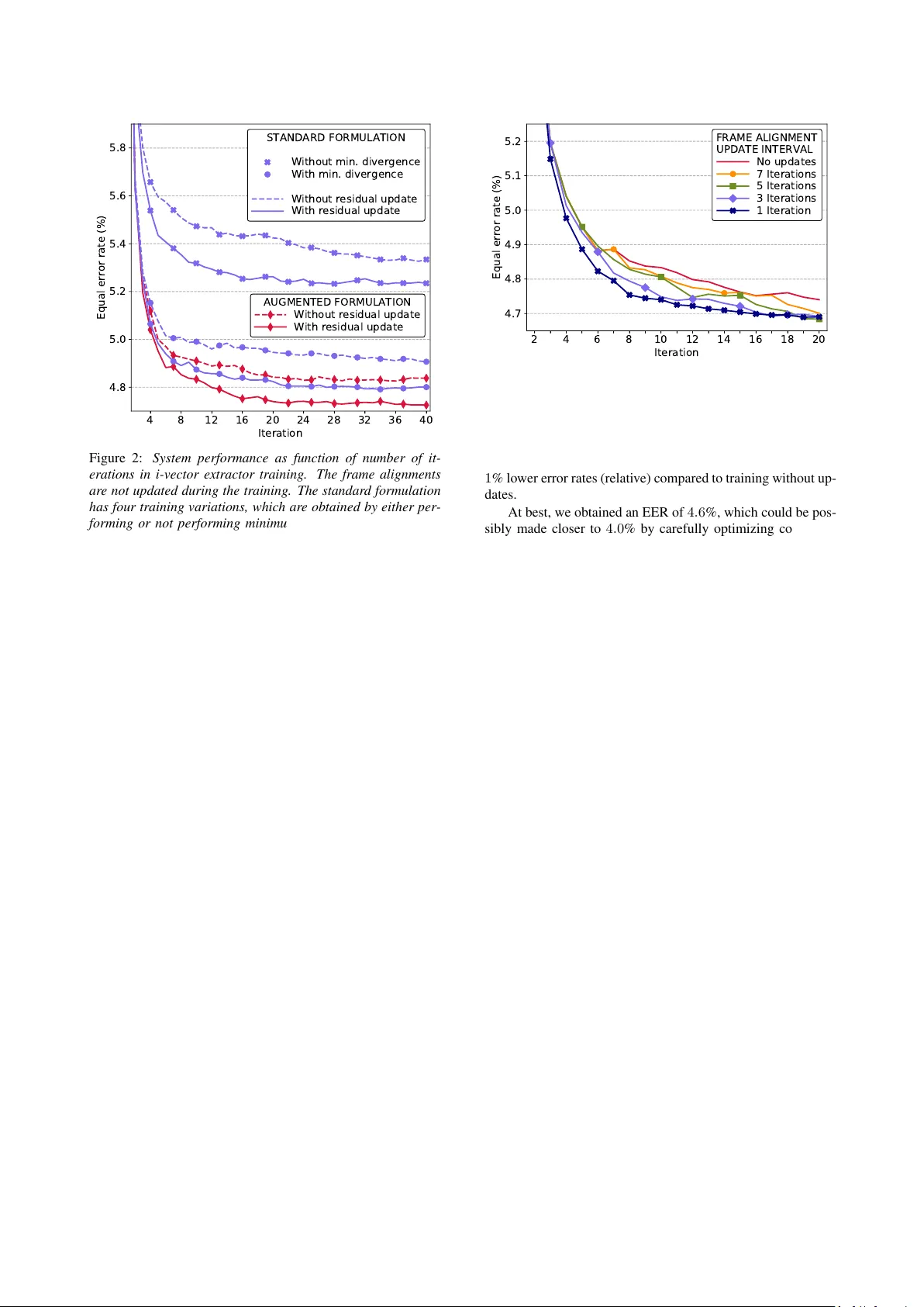
Unleashing the Unused P otential of I-V ectors Enabled by GPU Acceleration V ille V estman 1 , 2 , K ong Aik Lee 1 , T omi H. Kinnunen 2 , T akafumi K oshinaka 1 1 Biometrics Research Laboratories, NEC Corporation, Japan 2 Computational Speech Group, Uni versity of Eastern Finland, Finland vvestman@cs.uef.fi, k-lee@ax.jp.nec.com, tkinnu@cs.uef.fi, koshinak@ap.jp.nec.com Abstract Speaker embeddings are continuous-value vector representa- tions that allow easy comparison between v oices of speakers with simple geometric operations. Among others, i-vector and x-vector ha ve emerged as the mainstream methods for speaker embedding. In this paper , we illustrate the use of modern com- putation platform to harness the benefit of GPU acceleration for i-v ector extraction. In particular , we achiev e an accelera- tion of 3000 times in frame posterior computation compared to real time and 25 times in training the i-vector extractor com- pared to the CPU baseline from Kaldi toolkit. This significant speed-up allo ws the exploration of ideas that were hitherto im- possible. In particular , we show that it is beneficial to update the uni versal background model (UBM) and re-compute frame alignments while training the i-vector extractor . Additionally , we are able to study different variations of i-vector extractors more rigorously than before. In this process, we rev eal some un- documented details of Kaldi’ s i-vector extractor and show that it outperforms the standard formulation by a margin of 1 to 2% when tested with V oxCeleb speaker verification protocol. All of our findings are asserted by ensemble av eraging the results from multiple runs with random start. Index T erms : speaker recognition, PyT orch, factor analysis, total variability model 1. Introduction A decade ago, the i-vector speaker embedding was intro- duced [1]. Since its introduction, it has remained as a stan- dard solution for speaker recognition until recent years when it was excelled in many tasks by the deep neural network based embeddings [2, 3]. The recent developments are a result of the widespread interest among researchers to adopt deep learn- ing techniques in their research. The most recent rise of deep learning has been partially made possible by the year-by-year increasing computation resources [4], and especially the use of graphics pr ocessing units (GPUs) to harness the benefits of massiv e parallelism even with consumer le vel devices. While GPUs are hea vily adopted in deep learning, they can also be con veniently utilized for the traditional learning of gen- erativ e models such as the total variability model [5] underly- ing i-vector extraction. So far , this has been a largely unex- ploited possibility despite the fact that full-fledged i-vector ex- tractors tend to be slo w to train. The slo wness of training has of- ten forced many researchers to limit their experimental v alida- tion, for example by limiting the number of training iterations, or by relaying on the results from a single run with random initialization. In addition, simplifications and approximations of the model have been proposed to reduce the computational load [6, 7, 8]. For the current work, we utilize GPU to accelerate i-vector extraction and the total variability model training to alleviate the abov e limitations. The obtained speed-up allo ws us to study i- vector extractors in a more detailed manner than what has been possible pre viously . For example, we can train i-vector extrac- tors without any approximations for hundreds of iterations to study the optimal number of iterations to maximize the speaker recognition performance. In addition, we are able to obtain more reliable comparisons between different v ariations of ex- tractors by av eraging the results of multiple runs with different random initializations of the model. For instance, the extractor training can differ in terms of whether model parameters are r e- estimated using minimum diver gence criterion [9] and whether the residual cov ariance matrix of the model is updated. Further , we re-e xplore the idea of updating frame align- ments during the training of i-vector extractor , which could po- tentially enhance the model fit and the resulting speaker recog- nition performance. The idea of updating the alignments was originally presented in the context of eigenvoice modeling for automatic speech recognition [10], but has received limited at- tention in the context of i-vectors for speaker recognition. In eigen voice modeling, the alignment update is performed using speaker -dependent superv ectors, which is not suitable approach for speaker recognition as it would tend to model out the speaker information from the i-vectors. Instead, we update the global UBM mean supervector to realign the training data. In the experiments, we extensiv ely utilize our GPU re- implementation of Kaldi speech recognition toolkit’ s [11] i-vector extractor . The implementation in Kaldi has some spe- cial traits, which, to the best of our knowledge, hav e not been extensi vely documented. Most notably , in Kaldi’ s implemen- tation, the bias term is augmented to the total variability ma- trix [5], which causes some changes to the minimum diver gence re-estimation step and which also eliminates the need of central- izing Baum-W elch statistics [12]. As Kaldi is one of the most popular tools used for the speaker recognition research, we con- sider it worthwhile to document the main dif ferences of the tw o formulations in the following sections. 2. I-vector speaker embeddings W e compare two different formulations of the total variability approach [5] of joint factor analysis [13] to e xtract i-v ectors. In the total variability model, all of the v ariability in utterances is modeled using a single subspace only , without having separate subspaces to model speaker and channel ef fects. The first of the formulations is the original formulation [10, 14], which is commonly adopted in many av ailable speaker recognition toolkits [15, 16, 17]. The second formulation, im- plemented in the Kaldi speech recognition toolkit, is inspired by the subspace Gaussian mixture model [18]. This formula- tion differs from the standard one as it augments the bias term of the model to the factor loading matrix , which allo ws estimat- ing the bias term and the factor loading matrix jointly . Common to both formulations is the use of Baum-W elch statistics as defined in [14]. In this work, we denote the occu- pancy statistics, first order statistics, and the second order statis- tics for the Gaussian component c ( c = 1 , 2 , . . . , C ) as n c , f c , and S c , respectively . T o obtain unified presentation for the two formulations, we hereafter assume that the first and second or- der statistics are centered [19] for the standard formulation and not centered for the augmented formulation. 2.1. Standard formulation Follo wing the standard formulation, we model the mean vector of the c th Gaussian component of utterance u as µ c ( u ) = m c + T c ω ( u ) , (1) where m c is a bias term, matrix T c is a projection matrix, and ω ( u ) is a latent vector . The latent vector is shared among all the components and we assume that the prior over latent v ectors is standard normal. Further , the covariance matrix of the c th Gaussian is modeled as D c ( u ) = T c Φ ( u ) T T c + Σ c , (2) where Φ ( u ) is the posterior covariance matrix of the latent vector , and Σ c is the residual cov ariance matrix for compo- nent c [20]. The posterior covariance matrix Φ ( u ) and the mean vector φ ( u ) for the latent vector are obtained as Φ ( u ) = I + C X c =1 n c ( u ) T T c Σ − 1 c T c ! − 1 , (3) φ ( u ) = Φ ( u ) p + C X c =1 T T c Σ − 1 c f c ( u ) ! , (4) where p is the prior offset , which is 0 in the standard formula- tion. The model is trained iterati vely using an EM-algorithm, for which the update formulas for matrices T c and Σ c are given in [10]. In the beginning of training, the matrices T c are ini- tialized with random values drawn from the standard normal distribution. The initial bias terms m c and the residual covari- ance matrices Σ c are obtained as the means and covariances from universal backgr ound model (UBM) [12]. As the training progresses, the residual covariances get smaller as the first term of right-hand side of (2) starts to explain parts of the co variance structures of training utterances. 2.2. A ugmented formulation In the second formulation, we augment the bias terms m c into the matrices T c . This is done by assuming non-zero mean for the prior o ver the first elements of the latent v ectors. Then, equation (1) becomes µ c ( u ) = T c ω ( u ) , (5) where ω ∼ N ( p , I ) with p =  p 0 · · · 0  T , p ∈ R . Assuming that the Baum-W elch statistics are not central- ized, the equations (3) and (4) hold also for the augmented formulation. The EM update equations presented in [10] re- main the same as well 1 . It is worth to note that because of the augmentation, the update of matrices T c also updates the bias terms, which reside in the first columns of matrices T c . The model initialization differs slightly from the standard formulation. First, we set p = 100 (same as in the Kaldi im- plementation) and then we fill the first columns of the randomly initialized matrices T c with the values from the mean vectors of the UBM divided by p . 1 Although the residual cov ariance update implemented in Kaldi might seem different than in [10], the y can be shown to be equiv alent. 3. T raining enhancements The update step of the model training can hav e many varia- tions. The most basic one is to only update matrices T c , while also updating residual cov ariances Σ c giv es a slight improve- ment to the performance as we will demonstrate later . An- other way to improve the model is to apply minimum diver gence r e-estimation to make the empirical distribution of i-vectors close to standard normal [9, 14]. The minimum div ergence re- estimation is not quite as straightforward for the augmented for- mulation as for the standard one. T o the best of our knowledge, the procedure for the augmented formulation is not documented elsewhere than in the source code comments of Kaldi, hence we will provide the key details in the following. Finally , further improv ements can be obtained by realigning the training data during the training using the updated models. 3.1. Minimum diver gence re-estimation For the minimum div ergence re-estimation, we accumulate the sums h = 1 U U X u =1 φ ( u ) , (6) H = 1 U U X u =1 h Φ ( u ) + φ ( u ) φ ( u ) T i , (7) during the E-step. Then, a whitening matrix can be computed via eigendecomposition (alternatively , via Cholesky decompo- sition ) of the cov ariance matrix G = H − hh T . That is, if G = QΛQ T is an eigendecomposition of G , then the whiten- ing transform is obtained as P 1 = Λ − 1 2 Q T . Now , the up- date T upd c = T c P − 1 1 , has an effect of whitening the training i-vectors. In the standard formulation, the above update is sufficient for the minimum div ergence estimation. In the augmented for- mulation, howe ver , we need to apply another transform P 2 to the matrices T upd c to conform to the prior of fset assumption. In specific, after transforming i-vectors with P 1 and P 2 , they should remain whitened and only the first element (prior offset) of the projected mean vector P 2 P 1 h should be non-zero. One option for a transform that can satisfy the requirements set for P 2 is a reflection about a hyperplane that goes through the origin. This type of transform is kno wn as the Householder transform [21]. The Householder transform with a reflection hyperplane that is orthogonal to an unit length vector a is de- fined as P 2 = I − 2 aa T . (8) Now , the problem is to find a so that the projected mean vector is a scalar multiple of a unit vector e 1 =  1 0 · · · 0  . That is, P 2 P 1 h = b e 1 , b ∈ R . (9) It can be shown that one solution is a = α ˜ h + β e 1 , (10) where ˜ h is P 1 h normalized to unit length ( ˜ h = P 1 h / || P 1 h || ) and ( α = 1 √ 2(1 − ˜ h [1]) β = − α, (11) where ˜ h [1] is the first element of ˜ h . Now , the update T upd c = T c P − 1 1 P − 1 2 whitens and centers the training i-vectors with respect to the prior offset. Finally , the prior offset p is updated as follo ws: p = P 2 P 1 h . (12) 3.2. Realignment of training data T o compute the Baum-W elch statistics used in training, the frames of training utterances are first aligned to the components of the UBM by computing frame posterior probabilities. The posteriors and the Baum-W elch statistics are typically held con- stant during the training of i-vector e xtractor . In [10], the frame alignments of the training utterances are updated during the training of factor analysis model for auto- matic speech reco gnition (ASR). The realignment is done per speaker basis using adapted GMM means and covariances. In the application of speaker recognition, howe ver , this would be counterproductiv e as it would reduce the amount of speaker in- formation in the latent vectors. What we propose instead, is updating the UBM means with the updated bias terms m c and then using the updated UBM to realign the data, which can po- tentially lead to a better model fit. T o obtain the updated bias terms from the augmented formulation, we simply tak e the first columns of matrices T c and multiply them with p . In summary , the augmented model with posterior updates is trained by iterating ov er the following fi ve steps: 1. The computation of frame alignments and Baum-W elch statistics using the current UBM [12, 14]. 2. E-step: The computation of posterior means and co vari- ances for the latent vectors using (3) and (4) to accumu- late the required terms for the M-step. 3. M-step: The update of matrices T c followed by the up- date of residual cov ariances Σ c [10]. 4. Minimum divergence re-estimation: The update of matrices T c using the transforms P 1 and P 2 followed by the update of the prior offset p using (12). 5. If not the last iteration, the update of the mean vectors of the UBM with the first columns of matrices T upd c multi- plied by p . After the model has been trained, the updated UBM is used in the testing phase to compute the frame posteriors. 4. Experiments 4.1. Experimentation setup W e built the acoustic front-end of our systems on the basis of Kaldi [11] i-vector recipe for V oxCeleb [22, 23]. That is, we relied on Kaldi to extract MFCCs, to perform v oice activity de- tection (V AD), and to train the UBM. W e used the same settings as in the Kaldi recipe: The MFCC vectors are 72 -dimensional including delta and double-delta coefficients, and the UBM con- sists of 2048 components with full cov ariance matrices. Follo wing the Kaldi recipe, the UBM was trained using all of the data from the training parts of V oxCeleb1 and V oxceleb2 consisting of 1 277 344 utterances from 7325 speakers. The i- vector extractors were trained using the 100 000 longest utter- ances. T o train the scoring back-end, the Kaldi recipe uses the whole training data, while we utilized only the V oxCeleb1 pro- portion to speed up the experimentation. Although this reduced the number of training speakers from 7325 to 1211 , we did not observe de gradation in speaker verification performance 2 . After the i-vector extraction, we centered and length nor- malized the i-vectors. In addition, if minimum diver gence re- estimation w as not used, we also whitened the i-vectors be- fore length normalization. Then, we reduced the dimensionality 2 This might be explained by the fact that V oxCeleb1 has more reli- able speaker labels than V oxCeleb2 [23]. DISK CPU GPU Da t a loader 1: • Ba t ch es of fr ame s Da t a loader 2: • St a tis tics c omput a tion • Ba t ch es of ut t er anc es MFCCs , V AD la bel s Fr ame al ignm en ts Fr ame align men t : • Gauss ian sel ection • P os t eri or c omput a tion • P os t eri or thr eshol ding I - v ec t or e xtr act or • T r aining • E xtr action Figure 1: An overview of computational flow of frame align- ment, i-vector extraction, and model training using a GPU. T o keep the GPU memory r equirements constant, fixed size batc hes of frames and utterances are used for frame alignment and i-vector extr action, respectively . of i-vectors from 400 to 200 using linear discriminant anal- ysis (LDA) before subjecting them to probabilistic linear dis- criminant analysis (PLDA) scoring [24]. For testing, we used adopted the V oxCeleb1 speaker verification protocol, which consists of 37 720 trials with an equal number of tar get and non- target trials. W e ran the e xperiments on a server having Intel Xeon Gold 6152 CPU with 22 physical cores and NVIDIA Titan V GPU with 12 GB of memory . The file I/O operations were performed on a solid-state driv e (SSD). 4.2. GPU implementation In our implementations of frame alignment and i-vector e xtrac- tion, we utilized PyT orch [25] for GPU computations, SciPy ecosystem [26] for computations in CPU, and PyKaldi [27] for reading files stored in Kaldi format. The implementations use multiple CPU cores in parallel as data loaders, which load, pre- process, and feed the data to the GPU (Figure 1). The data loaders function in parallel with respect to the GPU to keep the GPU utilized all the time. For frame alignment, we use the same strategy as in Kaldi: First, to reduce the computational load, we use a UBM with di- agonal cov ariance matrices to select the top-20 Gaussian com- ponents with the highest frame posteriors for each frame. Sec- ond, we compute the posteriors with only the selected com- ponents using a full cov ariance UBM. Finally , we discard the posteriors that are less than 0 . 025 and we linearly scale the re- maining posteriors so that their sum equals to one. As a result, on av erage, only four Gaussian indices and the corresponding posteriors are stored to disk per frame. The Baum-W elch statistics used in i-vector extractor train- ing are computed in CPU, while the rest of the computation is done in GPU. The reason to compute statistics in CPU is as follows: For i-vector extraction implementation, it is natural to feed data in batches of utterances, and statistics provide a fixed size representation of utterances unlike the acoustic features. W e opted not to compute statistics beforehand as the disk usage would be excessiv e; instead we recompute them during each iteration of i-vector e xtractor training. W ith the settings laid out in Section 4.1, the GPU mem- ory usage for alignment computation is about 2 . 5 GB and for i- vector extractor training about 4 GB. The frame alignment can be done about 3000 times faster than real time (including I/O operations), and assuming that the alignments are ready in the disk, i-vectors can be e xtracted 10 000 times f aster than real 4 8 12 16 20 24 28 32 36 40 Iteration 4.8 5.0 5.2 5.4 5.6 5.8 Equal error rate (%) STANDARD FORMULATION Without min. divergence With min. divergence Without residual update With residual update AUGMENTED FORMULATION Without residual update With residual update Figure 2: System performance as function of number of it- erations in i-vector extractor training. The frame alignments ar e not updated during the training . The standard formulation has four training variations, which ar e obtained by either per- forming or not performing minimum diverg ence re-estimation and either updating or not updating r esidual covariance ma- trices. In the augmented formulation, the minimum divergence r e-estimation is always applied. Each curve is obtained as an averag e of five runs with differ ent random initial values of T c . time. By using the GPU re-implementation of Kaldi’ s i-vector extractor training, we were able to obtain 25 -fold reduction in the training times. This number was obtained by training both our GPU implementation and Kaldi’ s CPU implementation for fiv e iterations and measuring the elapsed times. The training using Kaldi utilized all the av ailable CPU cores in the server . 4.3. Speaker verification r esults W e began the experiments by comparing dif ferent variations of i-vector e xtractors to select the best one for further experiments with frame alignment updates. The results of the comparison are shown in Figure 2. W e observe the following: First, the minimum div ergence re-estimation to update the model hyper- parameters results in 7 . 5 – 9 % relativ e reduction in terms of equal error rate (EER). Second, the update of residual cov ari- ance matrices leads to 1 . 5 – 3 % relative reduction of error rates. Third, the augmented formulations obtain 1 – 2 % lower error rates (relative) than the standard formulations. Finally , we as- sert that 22 iterations are enough to reach the optimal speaker verification performance with the best performing e xtractors. As our results are av erages of five runs, indi vidual runs may con verge f aster than that. In addition, we confirmed that our as- sertion is correct by training the augmented model once for 200 iterations. Based on the first experiment, we continued to experiment with the realignment of training data using the augmented for- mulation with residual covariance matrix updates. W e varied the interval between the frame posterior updates ranging from updating on every iteration to updating only on ev ery sev enth iteration. W e display the results in Figure 3. The findings are two-fold: First, the more frequently the frame posteriors are updated, the faster the performance impro ves. Second, up- dating the posteriors, no matter how frequently , leads to about 2 4 6 8 10 12 14 16 18 20 Iteration 4.7 4.8 4.9 5.0 5.1 5.2 Equal error rate (%) FRAME ALIGNMENT UPDATE INTERVAL No updates 7 Iterations 5 Iterations 3 Iterations 1 Iteration Figure 3: P erformance of the augmented formulation for vary- ing intervals of frame alignment updates. The more often the alignments ar e updated, the faster the system performance im- pr oves. Eac h curve is obtained as an averag e of five runs with differ ent random initializations. 1 % lo wer error rates (relati ve) compared to training without up- dates. At best, we obtained an EER of 4 . 6 %, which could be pos- sibly made closer to 4 . 0 % by carefully optimizing configura- tions in various parts of the system. For comparison, the state- of-the-art system, using x-vectors, obtains EER of 3 . 1 % (re- ported in the Kaldi recipe). This is an expected performance difference between the i-v ector and x-vector systems [28]. 5. Discussion and conclusions W e have a couple of remarks from the practical aspect of the study . First, we found that by using the modern deep learning platforms, such as PyT orch, the implementation of GPU accel- erated algorithms for generative models is almost as straight- forward as it is with their non-GPU counterparts ( e . g . NumPy). The only concern is the limited amount of memory in GPUs. This limitation can be often circumvented by relying on the computational po wer of GPUs to recompute values that do not fit into the memory . The second remark concerns the update of the UBM means using the bias terms m c of the model. For this purpose, we only used the augmented formulation, but it can be done also with the standard formulation by updating the means in the min- imum diver gence step using a formula m upd c = m c + T c h [19]. Howe ver , we found that updating the means in this way did not work well together with residual cov ariance updates. In summary , the results of the study sho wed that the choice of the training algorithm for i-vector extractor matters as the relativ e change in equal error rate between the worst and the best variations was 11 . 4 %. For the optimal performance, our recommendation is to use the augmented formulation including the residual covariance updates and the updates of frame align- ments. Additionally we found that the extractors reach their maximum performance after 22 training iterations. 6. Acknowledgements This work was partially supported by Academy of Finland (proj. #309629) and by the Doctoral Programme in Science, T ech- nology and Computing (SCITECO) of the UEF . The authors at UEF were also supported by NVIDIA Corporation with the do- nation of T itan V GPU. 7. References [1] N. Dehak, “Discriminativ e and generative approaches for long- and short-term speaker characteristics modeling: application to speaker verification, ” Ph.D. dissertation, ´ Ecole de technologie sup ´ erieure, 2009. [2] D. Snyder, D. Garcia-Romero, D. Pove y , and S. Khudanpur, “Deep neural network embeddings for text-independent speaker verification. ” in Interspeech , 2017, pp. 999–1003. [3] D. Snyder , D. Garcia-Romero, A. McCree, G. Sell, D. Povey , and S. Khudanpur, “Spoken language recognition using x- vectors, ” in Pr oc. Odyssey 2018 The Speaker and Language Recognition W orkshop , 2018, pp. 105–111. [Online]. A vailable: http://dx.doi.org/10.21437/Odysse y .2018- 15 [4] I. Goodfellow , Y . Bengio, and A. Courville, Deep learning . MIT press, 2016. [5] N. Dehak, P . J. Kenny , R. Dehak, P . Dumouchel, and P . Ouellet, “Front-end factor analysis for speaker verification, ” IEEE T rans- actions on Audio, Speech, and Language Processing , v ol. 19, no. 4, pp. 788–798, 2011. [6] O. Glembek, L. Burget, P . Mat ˇ ejka, M. Karafi ´ at, and P . Kenn y , “Simplification and optimization of i-vector extraction, ” in 2011 IEEE International Conference on Acoustics, Speech and Signal Pr ocessing (ICASSP) . IEEE, 2011, pp. 4516–4519. [7] S. Cumani and P . Laface, “Factorized sub-space estimation for fast and memory effectiv e i-vector extraction, ” IEEE/ACM T ransac- tions on Audio, Speech, and Language Pr ocessing , vol. 22, no. 1, pp. 248–259, 2014. [8] L. Xu, K. A. Lee, H. Li, and Z. Y ang, “Generalizing i-vector esti- mation for rapid speaker recognition, ” IEEE/ACM T ransactions on Audio, Speech and Language Processing (T ASLP) , vol. 26, no. 4, pp. 749–759, 2018. [9] P . Kenny , “Joint factor analysis of speaker and session v ariability: Theory and algorithms, ” CRIM, Montr eal,(Report) CRIM-06/08- 13 , vol. 14, pp. 28–29, 2005. [10] P . Kenny , G. Boulianne, and P . Dumouchel, “Eigen voice model- ing with sparse training data, ” IEEE Tr ansactions on Speech and Audio Pr ocessing , vol. 13, no. 3, pp. 345–354, 2005. [11] D. Povey , A. Ghoshal, G. Boulianne, L. Burget, O. Glembek, N. Goel, M. Hannemann, P . Motlicek, Y . Qian, P . Schwarz et al. , “The Kaldi speech recognition toolkit, ” IEEE Signal Processing Society , T ech. Rep., 2011. [12] D. A. Reynolds, T . F . Quatieri, and R. B. Dunn, “Speaker veri- fication using adapted Gaussian mixture models, ” Digital signal pr ocessing , vol. 10, no. 1-3, pp. 19–41, 2000. [13] P . Kenny , G. Boulianne, P . Ouellet, and P . Dumouchel, “Joint factor analysis versus eigenchannels in speaker recognition, ” IEEE T ransactions on Audio, Speech, and Language Pr ocessing , vol. 15, no. 4, pp. 1435–1447, 2007. [14] P . Kenny , “ A small footprint i-vector extractor , ” in Odyssey , vol. 2012, 2012, pp. 1–6. [15] S. Madikeri, S. De y , P . Motlicek, and M. Ferras, “Implementation of the standard i-vector system for the kaldi speech recognition toolkit, ” Idiap, T ech. Rep., 2016. [16] A. Larcher, K. A. Lee, and S. Meignier, “ An extensible speaker identification SIDEKIT in Python, ” in 2016 IEEE Interna- tional Conference on Acoustics, Speech and Signal Pr ocessing (ICASSP) . IEEE, 2016, pp. 5095–5099. [17] S. O. Sadjadi, M. Slaney , and L. P . Heck, “MSR identity tool- box v1.0: A MA TLAB toolbox for speaker recognition research, ” 2013. [18] D. Povey , L. Burget, M. Agarwal, P . Akyazi, F . Kai, A. Ghoshal, O. Glembek, N. Goel, M. Karafi ´ at, A. Rastrow et al. , “The sub- space Gaussian mixture model—A structured model for speech recognition, ” Computer Speech & Language , vol. 25, no. 2, pp. 404–439, 2011. [19] P . Kenny , P . Ouellet, N. Dehak, V . Gupta, and P . Dumouchel, “ A study of interspeaker variability in speaker verification, ” IEEE T ransactions on Audio, Speech, and Language Pr ocessing , vol. 16, no. 5, pp. 980–988, 2008. [20] P . Kenn y , G. Boulianne, P . Ouellet, and P . Dumouchel, “Speaker adaptation using an eigenphone basis, ” IEEE transactions on speech and audio pr ocessing , vol. 12, no. 6, pp. 579–589, 2004. [21] A. S. Householder, “Unitary triangularization of a nonsymmetric matrix, ” Journal of the ACM (J ACM) , vol. 5, no. 4, pp. 339–342, 1958. [22] A. Nagrani, J. S. Chung, and A. Zisserman, “V oxCeleb: A large- scale speaker identification dataset, ” Pr oc. Interspeech 2017 , pp. 2616–2620, 2017. [23] J. S. Chung, A. Nagrani, and A. Zisserman, “V oxCeleb2: Deep speaker recognition, ” in INTERSPEECH , 2018. [24] D. Garcia-Romero and C. Y . Espy-W ilson, “ Analysis of i-vector length normalization in speaker recognition systems, ” in T welfth Annual Confer ence of the International Speech Communication Association , 2011. [25] A. Paszke, S. Gross, S. Chintala, G. Chanan, E. Y ang, Z. DeV ito, Z. Lin, A. Desmaison, L. Antiga, and A. Lerer, “ Automatic dif fer- entiation in PyT orch, ” in NIPS-W , 2017. [26] E. Jones, T . Oliphant, P . Peterson et al. , “SciPy: Open source scientific tools for Python, ” 2001–. [Online]. A vailable: http://www .scipy .org/ [27] D. Can, V . R. Martinez, P . Papadopoulos, and S. S. Narayanan, “Pykaldi: A Python wrapper for Kaldi, ” in IEEE Interna- tional Conference on Acoustics, Speech and Signal Pr ocessing (ICASSP) . IEEE, 2018. [28] D. Snyder , D. Garcia-Romero, G. Sell, D. Povey , and S. Khu- danpur , “X-vectors: Robust DNN embeddings for speaker recog- nition, ” in 2018 IEEE International Confer ence on Acoustics, Speech and Signal Processing (ICASSP) . IEEE, 2018, pp. 5329– 5333.