On Acoustic Modeling for Broadband Beamforming

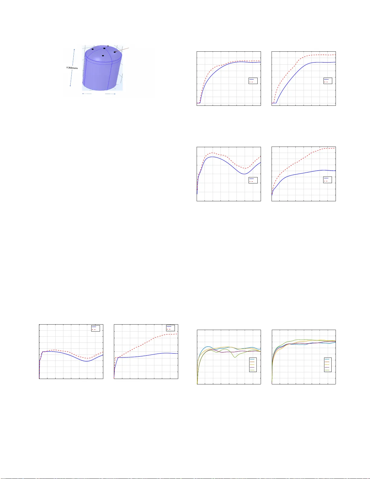
ON A COUSTIC MODELING FOR BR O ADB AN D BEAMFORMING Amit Chhetri, Mohamed Mansour , W ontak Kim, Guangdong P an Amazon Inc., USA ABSTRA CT In t his work, we describe limitations of the free-field propagation model for designing broadband beamformers for microphone arrays on a rigid surf ace. T o wards this goal, we describe a general frame- work for quantifying the micropho ne array performance in a gen- eral wav e-fi eld by directly solving t he acoustic wav e equation. The model utilizes Finite-El ement-Method (FEM) for ev aluating the re- sponse of the microphone array surf ace to background 3D planar and spherical wave s. The effectiv eness of the frame work is established by designin g and e v aluating a representativ e broadb and beamformer under realistic acoustic conditions. Index T erms — Beamforming, Microph one Arrays, Acoustics, FEM, W av e Equation. 1. INTRODUCTION Broadband beamforming with microphone array is a key signal pro- cessing module in many consumer electron ics produ cts, e.g., smart phones and smart speak ers [1–3]. The proliferation of mi crophone arrays due to decreasin g hardware cost and superior speech enhance- ment performance, has made broad band beam forming a ubiquitous embedded technology , and its performance has a critical impact on the ov erall system. A ke y requirement for broadband beamformin g i s to deliv er con- sistent performance across se v eral octaves of frequencies, e.g., 80 Hz - 8 K H z in the voice band case. Speech enhanceme nt is t ypically the system objec tiv e in most micropho ne arrays systems, rather than mere signal detection, as in the narro wband case. This po ses hard- ware and algorithmic challenges in the design of microphone arrays and the u nderlying beamforming pro cedure. Filter-and-Sum ( F &S) [4] h as been a standard approach for designing a b roadband b eam- former as an extens ion to a narrowban d beamformer by sti tching frequenc y-domain coefficients t hat are computed using narrowband beamforming techniques. Sev eral narro wband beamforming tech- niques, with different objectiv es and assumptions, b ecome standard design t echniques, e.g., Delay-and-Sum (D&S) [2, 5], Minimum- V ariance-Distortionless-Response (MVDR) [6, 7], Subspace meth- ods [3]. In t his work, we do not address a particular beamformer design algorithm. Rather, the emphasis is on the acoustic modeling, which is common among these techniques. Without loss of general- ity , MVDR-based F&S beamformer with a robustness co nstraint is used as a case study for our analysis. At a gi ven frequenc y and look- dir ecti on , the two ke y design parameters in almost all beamforming algorithms are the steering vector and the spatial coheren ce matrix. Proper design of these two parameters is the subject of this work. In Far-Field models, the acoustic wave is usually approximated by plane-wa v es [8], and the steering vector at th e direction/frequenc y of a plane wav e is de fined as the ob served acoustic pressu re at the differe nt microphones when the microphone array i s impinged with the plane-wav e. Near-Field steering ve ctors can similarly be approx - imated by acoustic spherical wa ves. The observed wa ve-field in the general cas e is the superposition of the incident w av e-field an d the scattered wav e-field. A typical approximation of the steering vecto r is the free-field approximation, which assumes sound propag ation in free-field (at the speed of sound in air) , and only the incident wa ve- field is consid ered. This app roximation is used almost unive rsally in the mi crophone array literature because it yields closed-form formu- lae tha t simplify be amformer ana lysis. The main issue of the free- field approximation is t hat it ignores the impact of t he device surface on the observ ed acoustic pressure, i.e., the scattered wav e-field. This impact, as will be shown , can significantly ch ange the m icrophone array behav ior at certain frequencies and angles. A possible remedy to this problem is to rely on anechoic lab measurements to quantify the de vice response to incident wav es. Ho we ver , this is a time-consuming and high -cost solution, and im- perfect e xperimental sett ings cou ld lead to noticeable modeling er- rors, especially in near-field cases. In this work, we describe a simulation-based approach for acoustic modeling of microphone ar- ray on rigid surf ace by solving the Helmholtz wa ve equation using Finite-Element-Method (FE M) with a background wa ve-field that matches the i ncident wav e-field [9]. Prior works that studied the impact of scattered field on micropho ne arrays used spherical har- monic decomposition for specific form-factors (e.g. sphere, cylin- der) [10–12] (and refere nces, therein). Ho we v er , these methods are restrictiv e in the choice of dev ice form-fa ctors (e. g. do not inc lude modern smart-speak er form-factors) and beamforming techniques. In comparison, the FEM method proposed in this paper provides three notable contribu tions: (i) a methodology to compute the steer- ing vector f or microphone arrays mounted on solid hard surfaces without the nee d for expensi ve anech oic chambe r measurem ents, (ii) ability to design any type of beamformer that r el i es on steering vec- tors; these include MVDR beamformer [2], linearly constraine d min- imum v ariance (LCMV) beam former [13, 14], and polynomial beam- former [15], and (iii) extension of the proposed method to generic de vice form-factors that are used for smart speakers. The f ollo wing notations are used thro ughout the paper . A bo ld lo wer-case lett er de notes a column v ector , while a bold uppe r-case letter denotes a matrix. A T and A H denote the transpose and con- jugate transpo se, r espectively , of A , and A m,n is the matrix entry at position ( m, n ) . Θ , ( θ, φ ) T denotes the polar and azimuth an- gles, respec tiv ely , in a spherical coordinate system. M always refers to the number of microphones . Ψ ( ω ) denotes the noise coherence matrix, of size M × M , at frequency ω (the depende ncy on ω is dropped whene v er it is clear from t he context). Additional notations are introduced when needed. 2. BA CKGR OUND 2.1. W av e Equ ation The acoustic wav e equation [16 ] is the go verning equation for t he propagation of sound wav es at equilibrium in elasti c fluids, e.g., air . The homoge nous wav e equation has the form ∇ 2 ¯ p − 1 c 2 ∂ 2 ¯ p ∂ t 2 = 0 (1) where ¯ p ( t ) is the acoustic pressure, and c is the speed of sound in the medium. In this wo rk, w e consider only the practical case of homogen ous fl uid with no viscosity . In practice, the wa ve equation is usually solved in the frequen cy domain using the Helmholtz equation to find p ( ω ) : ∇ 2 p + k 2 p = 0 (2) where k , ω /c is the wav e number . At steady state, the time-domain and fr equency-domain solutions are Fourier pairs [17]. In our mod- eling, we wo rk only with the homogenou s Helmholtz equation und er v arious boundary conditions. The boun dary conditions are deter- mined by t he geometry and the acoustic impedance of the different boundaries. W e assume the device has a rigid surf ace, therefore, it is modeled as a sound hard boundary . 2.2. Beamf orming Strategies Beamforming is a microphone-array sign al processing technique that al l o ws emphasizing the user’ s speech from a desirable look- direction (LD) while suppressing interferences from other direc- tions. Here, we process microp hone elemen ts such that the signals arrivin g from look-direction are combine d in-phase, while signals arrivin g from other directions are combined out-of-phase. Denote the position of the m -th microphone by r m , and the si gnal acquired at the m -th microphone for frequenc y ω by x ( w , r m ) . T hen, the signal acquired by the microphone array can then be expressed as: x ( ω , r ) = [ x ( ω , r 1 ) x ( ω , r 2 ) . . . x ( ω , r M )] T . (3) Denoting the spectrum of the desired source signal by s ( ω ) and the ambient noise captured by the mi crophone array as n ( ω ) , we can express x ( ω , r ) as: x ( ω , r ) = v ( ω , Θ ) s ( ω ) + n ( ω ) , (4) where, v ( ω , Θ) , [ v 1 ( ω , Θ ) v 2 ( ω , Θ ) . . . v M ( ω , Θ)] is the fre- quenc y and angle-dependent st eering vector . The beamformer design in v olves computation of complex- v alued weights for each frequenc y and microphone denoted by w ( ω ) , [ w 1 ( ω ) w 2 ( ω ) . . . w M ( ω )] T , which are t hen applied to x ( ω , r ) to obtain the beamformer output y ( ω ) : y ( ω ) = w H ( ω ) x ( ω , r ) . (5) W e are interested in using FEM modeling for the design of F&S beamformers t hat can be express ed as a constrained optimization problem, and the solution to which provides t he optimal beamformer filters. This covers various F&S beamformers like MVDR, maxi- mum SNR, and LCMV beamformers [13]. In this work, we use, without l oss of generality , the MVDR beamformer with a robu stness constraint to present our analysis. 2.3. Beamforming Metrics W e use three metrics to assess the performance: arr ay gain (A G), white noise gain (W NG) [2], and microphone array channel capac- ity (MA CC) [18]. The A G metri c is defined as the improvement in signal-to-noise-ratio (SNR) of fered by the beamformer: AG ( ω ) , S N R out ( ω ) S N R in ( ω ) . After some algebraic manipulations, one can sho w t hat [2]: A G ( ω, Θ LD ) = | w H v ( ω , Θ LD ) | 2 w H Ψ ( ω ) w , (6) where Θ LD denotes the look-d irection, and Ψ , Λ /β is the nor- malized noise correlation matrix with Λ m,q = Z π 0 Z 2 π 0 v m ( ω , Θ ) v ∗ q ( ω , Θ ) σ 2 N ( ω , Θ) sin( θ ) dθ dφ, (7) where σ 2 N ( ω , Θ ) denotes the d istribution of noise po w er as a func- tion of ω and Θ , and β = Z π 0 Z 2 π 0 σ 2 N ( ω , Θ) sin( θ ) d θ dφ. (8) The WNG metric is the SNR imp rov ement provide d by the beam- former when the noise compon ents at the microph ones are statisti- cally independent [2]: WNG ( ω , Θ LD ) = | w H v ( ω , Θ LD ) | 2 w H w . (9) The MACC me tric [18] aims at pro viding a characterization of the microphone array that is independent of the beamforme r realization. It is analogous to MIMO channel capacity i n wireless co mmunica- tion. If t he source location is known, then the MA CC is defined as MA CC ( ω , Θ LD ) , log  1 + P k S − 1 2 U H v ( ω , Θ LD ) k 2  (10) where USU H is the singular v alue decomp osition of Ψ , and P is the input powe r . 3. A COUSTIC MODELING 3.1. Acoustic Plane-W av es Acoustic plane wav es constitute a powerful tool for analyzing t he wa ve equation, and it pro vides a goo d approximation of the w av e- field emanating from a fa r-field point source [11]. The acoustic pres- sure of a plane-wav e wit h vector wave number k is defined at a point r in the 3D space as: p ( k ) , p 0 e − j k T r (11) This is a solution of the inhomogeneo us Helmholtz equation with a far p oint source, where k k k = k (note that, for a giv en k in the Helmholtz equation, there are two de grees of freedom in ch oosing k ). F urther , a general solution to the homogenous Helmholtz equa- tion can be approximated by a linear superposition of plane w av es of differe nt angles [17, 19–21]. These properties render acoustic plane- wa ves a key t ool in designing far-field beamforming for microphone arrays, where the microphone array response to each plan e wav e pro- vides a sufficient set for the beamformer design. The total wavefield at each microphon e of the microph one array when an incident plane-w av e p i ( k ) impinges o n the de vice has the general form: p t = p i + p s (12) where p t and p s refer to the t otal and scattered wavefield respec- tiv ely . The total wave field, p t , at each microphone is computed by inserting (12) in the Helmholtz equation (2) and solving for p s with appropriate boundary conditions. The details of this modeling are described in section 3.2. It is evident from (11) that an incident plane-wa v e does not hav e magnitude information, and it is fully pa- rameterized by it s phase. This is not true for the scattered wavefield, p s which represents t he reflections/diffractions du e to the ri gid de- vice surface. This magnitude information in p s is critical in resolv- ing phase ambiguity due to microphone array geometry . If the microphone array is compo sed of discrete microphones in space, and the area of each micro phone is much smaller than t he wa veleng th, then a reasonable approximation i s to set p s = 0 in (12). T his is referred to as fr ee-field approximation . In this case, the total wav efield, p t , is fully determined b y the waven umber k in (11), and the ( x, y , z ) coordinates of each microphone. It is obvio us that, free-field approximation is not accurate if t he microphone ar- ray is on a rigid surface. Neverthe less, this approximation h as been utilized almost uni versally i n the l i terature for acoustic mo deling in beamformer design. In the followin g section, we show that the free- field approximation does not prov ide a good approximation of the total field under important practical cases. 3.2. FEM Mod eling The modeling objectiv e is to compute the total sound field in (12) at ea ch microphon e when the de vice is impinged by a plane wav e. This resembles physical measurement i n anech oic room with a d is- tant point source. FEM is one of the standard approache s for so lv- ing the Helmholtz equation numerically . In our case, we need t o solve the Helmholtz equation for the total w av efield at all freq uen- cies of i nterest with a backgr ound plane wave . T he de vice surface is modeled as sound hard boundary . The microphone is modeled as a point recei ver on the surf ace if the microphone su rface area is much smaller than t he wa velen gth, otherwise, i ts response is com- puted as the integral of the acoustic pressure ov er its area. T o ha v e a true backgroun d plane-wa ve, the external boundary should be open and non-reflecting. In our model, the dev ice is enclosed by a closed boundary , e.g., a cy linder or a spherical surface. T o mimic open- ended boundary , there are two choices: (i) Matched bound ary whose impedance is matched to the air impedance at the frequenc y of inter - est, (ii) Perfectly matched layer , which defines a special absorb ing domain that eliminates reflection an d refractions in the interna l do- main that encloses the device [22]. The merits of each approach is be yond the scope of this paper . The FEM solves for p t in (12), which is equi v alent to solving for only the scattered field, p s , af- ter inserting background plane wav e model (11) in the Helmholtz equation. The acoustics module of COMSOL multiphysics pack- age [23] i s used for t his FEM nume rical solution, and the simulation is rigorously validated with exact and measured r esults on different form-factors. For example, in Fig. 1, we show the total pressure field of two microphones on a spherical surf ace with analytical a nd simulated solution. Both amplitude an d phase responses match e x- cellently wi t h t he analytical solution [24]. Further , in Fig. 2, we sho w an ex ample of simulated and measured acoustic pressure of a rectangu lar microphone array mounted on a slanted cube. In the plot, we show the inter-channel response, i.e., { H i ( ω ) /H r ( ω ) } i 6 = r , where r is a reference microphone. The phase dif ference between simulated and measured respo nses is linear , which is ex pected when the positions of the device in both cases are not perfectly aligned. For more comparisons b etween simulated/theoretical a nd measured acoustic pressure responses, one may refer to [25, 26]. Note that, the abov e procedure is not limited to p lane-wa ve as we only need to specify the backgrou nd pressure field, which could be, for exam ple, spherical wav e for near-field modeling. T he proce- dure i s repeated f or a grid of frequency and i ncident angles to build a dictionary of total pressure { p t ( ω , θ , φ ) } ω ,θ,φ that is used in sub- sequent analysis. 1000 2000 3000 4000 5000 6000 7000 8000 Frequency (Hz) 0 0.5 1 1.5 2 2.5 Amplitude mic1-FEM mic1-Exact mic2-FEM mic2-Exact 1000 2000 3000 4000 5000 6000 7000 8000 Frequency (Hz) -4 -2 0 2 4 Phase (radians) mic1-FEM mic1-Exact mic2-FEM mic2-Exact Fig. 1 : Compari son of FEM and analyti cal soluti ons for spherical surfa ce of radius 5 cm. T op: magnitu de response, bottom: pha se response. Mic 2 is in the middl e of sphere fac ing th e inci dent wa ve; Mic 1 is fac ing aw ay from it. 0 1000 2000 3000 4000 5000 6000 7000 Freq (Hz) -4 -2 0 2 Magnitude (dB) (th,ph) = (210.0,90), mth=30 0 1000 2000 3000 4000 5000 6000 7000 Freq (Hz) 0 0.5 1 1.5 2 Phase (rad/ π ) Fig. 2 : Normalized acoustic pressure of a rectangul ar microp hone array on a slanted cub e for simulate d and measure d cases for a background plane wa ve at directi on ( θ, φ ) = (90 ◦ , 210 ◦ ) (simulated response is in dotted lines, measured response in solid lines, with dif ferent colors for differe nt micro- phones). T op: magnitude, bottom: phase differe nce 4. ANAL YSIS OF FREE-SP A CE BEAMFORMING T o i llustrate the benefits of FEM modeling, we use the MVDR beam- former with a robustness constraint, formu lated as a constrained con- ve x optimization problem [14]: b w = arg min w w H Ψ w such that w H v ( ω , θ LD ) = 1 , | w H v ( ω , Θ LD ) | 2 w H w ≥ γ , (13) where the first constraint i s called the distorti onless constraint [2 ], and the second constraint is the WNG constraint, which imposes ro- bustne ss in the beamformer design t hat can be controlled through γ [14]. Further , the WNG constraint enables a more fair compar - ison between the total and f r ee-field beamformer designs because the W NG is bounded in both cases. Without loss of generality , we assume a spherically diffuse noise field. The optimization problem in (13) is solved using a con vex optimization solver to obtain the beamformer weights b w . Note that the proposed F E M-model based method can be simi l arly extende d to other beamformer designs like the MVDR [2], LCMV [ 13], and polynomial beamformer [15]. !"# $$ $%&'()*(+, Fig. 3 : Simulation setup for FEM-based beam forming. T he form- factor is a combination of a cylindrical bottom and a top surface with a spherically-curve d shape. 4.1. Analysis M ethodology The MVDR solution can be obtained from (13) by usin g v i and v t as steering vectors for free-field (FF) and total-fi eld ( TF), respec- tiv ely . T o compute Ψ , we use analytical method f or can onical device shapes, such as fi nite cylinder and sphere [24]. For a general de vice shape, the FEM tool is used to simulate the steering vectors for a uniform grid of azimuth and polar ang les. Then, Ψ is numerically computed from (7) and (8), with σ 2 N ( ω , Θ) = 1 for the sp herically diffu se noise field. W e now compare the performance of MVDR beamformer de- signed using FF and TF assumptions. For our study , we use the setup in Fig. 3, which has 5 microphon es on the top of a cylin- der of height 130 mm and diameter of 70 mm; the top surfa ce of the cylinde r has a spherically-curv ed shape. This surface does not hav e a closed-form solu tion for the Helmholtz equation, which ne- cessitates the use of the pro posed FEM method. The origin of the coordinate system coincides with the center microphone with z ax is pointing upw ards, and the x - y plane parallel to the bottom f ace of the cylinde r . The coordinates of the microphones are: ( x, y , z ) = { ( r o , 0 , z o ) , (0 , r o , z o ) , ( − r o , 0 , z o ) , (0 , − r o , z o ) , (0 , 0 , 0) } , where r o = 30 mm and z o = − 3 mm. Lastly , we set γ = − 25 dB. 4.2. Results W e ev aluate the microphone array metrics under Free Fi el d (FF) and T otal Field (TF) setups for the array in Fig. 3 at two arriv al angles: ( θ , φ ) = (90 ◦ , 0 ◦ ) and (30 ◦ , 0 ◦ ) . The results are summarized in Figs. 4-6 f or the three performance metrics. 0 1000 2000 3000 4000 5000 6000 7000 8000 Frequency (Hz) 0 2 4 6 8 10 12 14 16 18 Array Gain (dB) FF TF (a) ( θ, φ ) = (90 ◦ , 0 ◦ ) 0 1000 2000 3000 4000 5000 6000 7000 8000 Frequency (Hz) 0 2 4 6 8 10 12 14 16 Array Gain (dB) FF TF (b) ( θ , φ ) = (30 ◦ , 0 ◦ ) Fig. 4 : A G performan ce showing the dif ference between FF and TF . Note ho w the array gain is higher , especially at high fr equencies. At θ = 90 ◦ , i.e., x - y plane, the TF case i s slightly better for the A G and MA CC , but the WNG performance f or the TF case is better than t he FF case. This is explained by noting that the steering vectors in the TF case have v ariations in both phase and amplitude (ov er 0 1000 2000 3000 4000 5000 6000 7000 8000 Frequency (Hz) -25 -20 -15 -10 -5 0 5 10 15 White Noise Gain (dB) FF TF (a) ( θ , φ ) = (90 ◦ , 0 ◦ ) 0 1000 2000 3000 4000 5000 6000 7000 8000 Frequency (Hz) -25 -20 -15 -10 -5 0 5 10 15 White Noise Gain (dB) FF TF (b) ( θ , φ ) = (30 ◦ , 0 ◦ ) Fig. 5 : WNG performance. Note that ev en wi t h the higher array gain from Fig. 4, the WNG is better for the T F configuration. 0 1000 2000 3000 4000 5000 6000 7000 8000 Frequency (Hz) 2.5 3 3.5 4 4.5 5 5.5 Channel Capacity (bits) FF TF (a) ( θ , φ ) = (90 ◦ , 0 ◦ ) 0 1000 2000 3000 4000 5000 6000 7000 8000 Frequency (Hz) 2 2.5 3 3.5 4 4.5 5 5.5 6 6.5 Channel Capacity (bits) FF TF (b) ( θ , φ ) = (30 ◦ , 0 ◦ ) Fig. 6 : MA CC performance, which corresponds well with the A G performance in Fig. 4. microphones) in comparison to the FF case, which only has phase v ariations. The amplitude v ariations increase t he spatial div ersit y for the TF case, which can be used to improv e the spatial directivity of the beamformer . At θ = 30 ◦ , the TF case has WN G performance better than the FF over the full f r equency range; the AG for TF case is noticeably better than FF case for all frequencies, and significantly better for frequencies beyon d 2 kHz. Note that the WNG curves are lo wer-boun ded by − 25 dB, because of the WNG con straint specified in (13). Note also that in all cases, the MA CC for the T F case is noticeably better than the FF case, because the FF case i gnores the magnitude information , which provides in v aluable characterization of the look direction. 0 1000 2000 3000 4000 5000 6000 7000 8000 Frequency (Hz) 20 30 40 50 60 70 80 90 100 110 Sound Pressure Level (dB) 1 2 3 4 5 (a) ( θ , φ ) = (90 ◦ , 0 ◦ ) 0 1000 2000 3000 4000 5000 6000 7000 8000 Frequency (Hz) 20 30 40 50 60 70 80 90 100 110 Sound Pressure Level (dB) 1 2 3 4 5 (b) ( θ , φ ) = (30 ◦ , 0 ◦ ) Fig. 7 : Magn itude of scattered wav efield, p s , (in dB) at two p lane wa ve angles. The big dev iation of the FF performance at θ = 30 ◦ is attri buted to the magnitude of the scattered wav efield (which is ignored in the FF case). This is i l lustrated in Fig. 7, where we sho w the magni- tude of the scattered wa vefield at the fi ve micro phones at both an- gles (where the background plane wav e has the same mag nitude in both cases). Note that, the scattered wa vefield at θ = 30 ◦ is approx- imately 10 dB stronger than θ = 90 ◦ especially at high frequencies, which is manifested clearly in the corresponding AG/WNG/MA CC behav ior . This significant de viation of the free-fi eld case demon- strates the limitation of this modeling and the necessity of incor- porating the scattered fi el d compone nt through FEM modeling for beamformer design. 5. CONCLUSION AND FUTURE WORK The free-fiel d model does not provide accurate modeling for broad- band beamformer design, especially when the scattered wavefield is significant. Therefore, designing beamformer metrics based on free-field modeling results in suboptimal performance. T o mitigate this issue, we described a simulation-based frame work for modeling the total wa ve field, which is sho wn to noticeably improv e the beam- former design. T he model is univ ersal for any de vice surface, and it could be used for both near-field and far-field modeling by comput- ing the steering vectors of sph erical and plane w av es, respecti vely . Future work will utilize the results of this work to de velop novel de- sign techniques for broadban d beamformer and generic form-factors that are based on this realistic micropho ne arr ay modeling [27]. Ad- ditionally , we e xpand the array processing metrics, and sho w a close matching of simulated and measured beampatterns for our proposed method [27]. 6. REFERENCES [1] Amit Chhetri, Philip Hilmes, Trausti Kristjansson, W ai Chu, Mohamed Mansour , Xiaoxue Li , and Xianxian Zhang, “Mul- tichannel Audio Front-End for Far-Field Automatic Speech Recognition, ” in 2018 26th Europ ean Signal P r ocessing Con- fer ence (EUSIPCO) . IEEE, 2018, pp. 1527–1531. [2] Michael Brandstein and Darren W ard, Micr ophone arrays: sig- nal pr ocessing tec hniques and app lications , Springer Science & Business Media, 2013. [3] Jacob Benesty , Jingdong Chen, and Y iteng Huang, Micr o- phone array signal pr ocessing , vol. 1, Springer Science & Business Media, 2008. [4] Otis Lamont Frost, “ An algorithm for li nearly constrained adapti ve array processing , ” Proce edings of the IE E E , vol. 60, no. 8, pp. 926–935, 1972. [5] Dan E Dud geon, “Fundamen tals of digital array processing, ” Pr oceeding s of the IE E E , vol. 65, no. 6, pp. 898–904, 1977. [6] Jack Capon, “High-reso lution frequency-wa v enumber spec- trum analysis, ” Pr oceeding s of the IEEE , vol. 57, no. 8, pp. 1408–1 418, 1969. [7] Henry Cox, Robert Zeskind, an d Mark Owen, “Robust adap- tiv e beamforming, ” IE EE T ransa ctions on Acoustics, Speech, and Signal Pr ocessing , vol. 35, no. 10, pp. 1365–1376, 1987. [8] Heinrich K uttruf f, Room acou stics , CRC Press, fourth edition, 2000. [9] Stig Larsson and V idar Thom ´ ee, P artial differ ential equations with numerica l methods , v ol. 45, Springer S ci ence & Business Media, 2008. [10] Dmit r y N Z otkin, Nail A Gumerov , and Ramani Duraiswami, “Incident field recov ery for an arbitrary-shaped scatterer, ” in Acoustics, Speech and Signal Proc essing (ICASSP), 2017 IEEE International Confer ence on . IEEE , 2017, pp. 451–455. [11] Heinz T eutsch, Modal arr ay signal pr ocessing: principles and applications of acoustic wave field decomposition , vo l. 348, Springer , 2007. [12] Boaz Rafaely , Fundamentals of spherical array pr ocessing , vol. 8, Springer , 2015. [13] H. L. V an T rees, Optimum Array Pro cessing , Wile y , New Y ork, 2002. [14] E dwin Mabande , Adrian S chad, and W alt er Kellerman n, “De- sign of robu st superdirectiv e beamformers as a con vex opti- mization problem, ” in Acou stics, Sp eech and Sign al P r ocess- ing, 2009. ICASSP 2009. IEEE International Confere nce on . IEEE, 2009, pp. 77–80. [15] E Mabande and W alter K ellermann, “Design of robu st polyn o- mial beamformers as a con v ex optimization problem, ” in Proc. IEEE Int. W orkshop Acoustic Echo, Noise Contr ol (IW AENC) , 2010, pp. 1–4. [16] L awrence E Kinsler , Austin R Frey , Alan B Coppens, and James V Sanders, F undamentals of acoustics , Wile y , third edition, 1982. [17] E arl G W illi ams, F ourier acoustics: sound radiation and nearfield acoustical hologr aphy , Academic press, 1999. [18] Mohamed F Mansour , “Information measures for microphone arrays, ” arXi v pr eprint arXiv:1801.101 28 , 2018. [19] Andrea Moiola, Ralf Hiptmair, and I Perugia, “Plane wav e ap- proximation of homogeneous helmholtz solutions, ” Zeitschrift f ¨ ur angewa ndte Mathematik und Physik , vol. 62, no. 5, pp. 809, 2011. [20] Orhan Y ilmaz and M T urhan T aner , “Discrete plane-wav e de- composition by least-mean-square-error method, ” Geophysics , vol. 59 , no. 6, pp. 973–982 , 1994. [21] E mmanuel Perre y-Debain, “Plane wav e decomposition in the unit disc: Con vergen ce estimates and co mputational a spects, ” J ournal of Computational and Applied Mathematics , vol. 193, no. 1, pp. 140–156, 2006. [22] Jean-Pierre Berenger , “ A perfectly matched layer for the ab - sorption of electromagnetic wa ves, ” Journal of computational physics , vol. 114 , no. 2, pp. 185–200, 1994. [23] COMSOL Multiphysics , “ Acoustic modu le–user guide , ” 2017 . [24] John J Bowman, Thomas B S enior , and P iergiorg io L Uslenghi, Electr oma gnetic and acoustic scattering by simple shapes , North-Holland Publishing Company , 1970. [25] F rancis M Wiener , “T he diffraction of sound by rigid disks and rigid sq uare plates, ” The J ournal of the A coustical Society of America , vol. 21, no. 4, pp. 334–347, 1949. [26] RD Spence, “The dif fraction of sound by circular disks and apertures, ” The Journa l of the Acoustical Society of America , vol. 20 , no. 4, pp. 380–386 , 1948. [27] Guangdong Pan, W ontak Kim, Sav askan Bulek, Amit Chhetri, and Mohamed Mansour , “ A study on acoustic modeling for microphone array beamforming, ” pr e-print , 2019.