Age-Minimal Transmission for Energy Harvesting Sensors with Finite Batteries: Online Policies

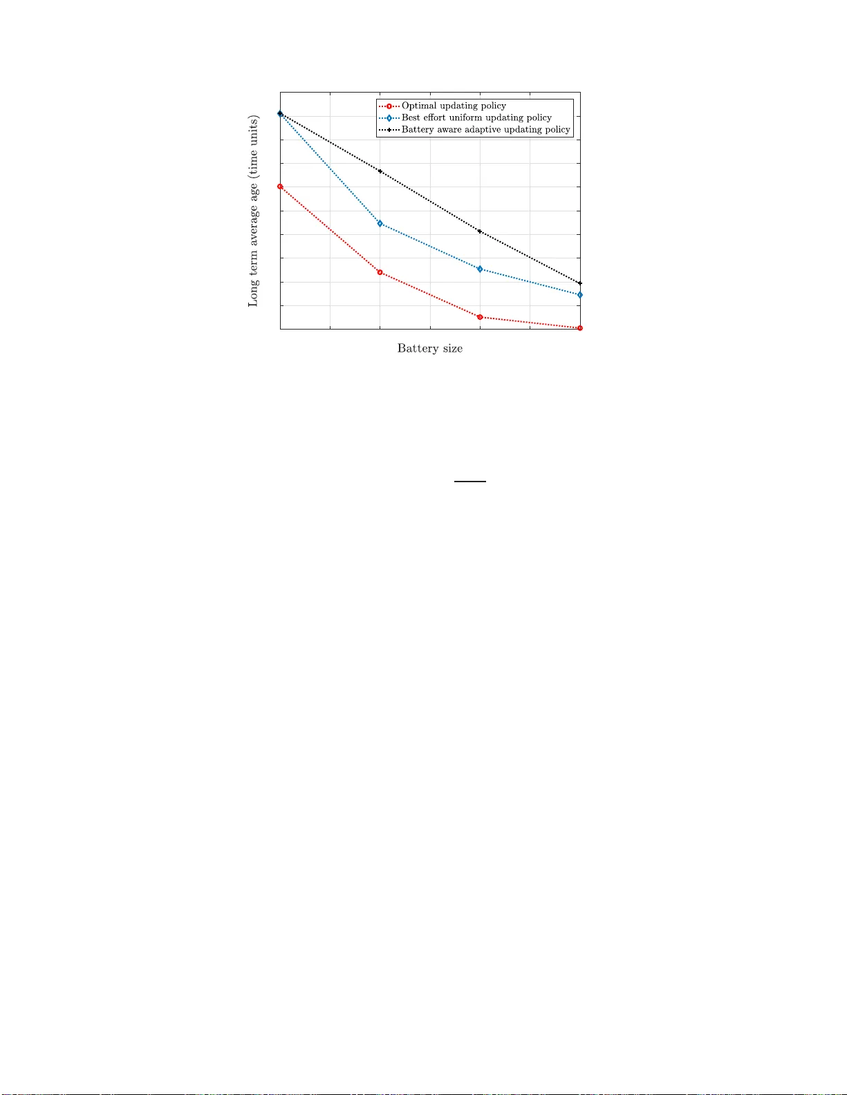
Age-Minimal T ransmission for Energy Harv esting Sensors with Finite Batteries: Online P olicies ∗ Ahmed Arafa , Jing Y a ng, Senn ur Ulukus, and H. Vincen t P o or Ma y 10, 2019 Abstract An energy-harv esting s en sor nod e t hat is sending status up dates to a destination is considered. The sensor is equip p ed with a battery of finite size to sa v e its incoming energy , and consumes one unit of energy p er status up date transmission, whic h is deliv ered to the destination ins tantly o ver an err or-free c h annel. The setting is online in whic h the harveste d energy is rev ealed to the sensor causally o ve r time after it arriv es, and the goal is to d esign status up date transmission times (p olicy) suc h that the long term av erage age of information (AoI) is min imized. The A oI is defin ed as the time elapsed since the latest up date has reac h ed at the d estination. Tw o energy arr iv al mo dels are considered: a r andom b attery r e char ge (RBR) mo del, and an incr emental b attery r e char ge (IBR) mo del. In b oth mo dels, energy arrive s according to a P oisson pro cess with unit rate, with v alues that completely fill u p the b attery in the RBR mo del, and with v alues that fill up the battery incremen tally in a unit-by-unit fashion in the IBR mo d el. T he key appr oac h to c h aracterizing the optimal status up date p olicy for b oth mo dels is sho wing the optimalit y of r enewal p olicies , in w h ic h the inte r-up d ate times follo w a renewal p ro cess in a certain man n er th at dep ends on the energy arriv al mo del and the battery size. It is then sho wn that the optimal renewa l p olicy has an energy-dep endent thr eshold stru cture, in whic h th e sensor sends a status up date only if the AoI gro ws ab o ve a certain thr eshold that d ep ends on the energy a v ailable in its battery . F or b oth the random and the incremen tal b attery r ec harge mo dels, the optimal energy-dep endent thresholds are charac terized e xplicitly , i.e., in closed-form, in terms of the optimal long term a ve rage AoI. It is also shown that th e op timal thresh olds are monotonically decreasing in the energy a v ailable in the battery , and that the smallest threshold, whic h comes in effect when the b attery is full, is equal to the optimal long term a ve rage AoI. ∗ Ahmed Arafa and H. Vincen t Poor are with the Electrical E ngineering Depar tmen t, Princeton University , NJ 08544 . Jing Y a ng is with the Scho ol o f Electr ical E ngineering and Computer Science, The Pennsylv ania State Universit y , P A 16802 . Sennur Ulukus is w ith the Department of Ele ctrical and Computer Eng ineer- ing, University o f Mar yland Colleg e Park, MD 2 0742. Emails: aar afa@princ eton.e du , yangjing@psu.e du , ulukus@u md.e du , p o or@princ eton.e du . This w ork is presented in pa rt in the 20 18 Information Theory and Applications W or k shop [1], and in the 2 018 International Conference on Communications [2]. 1 1 In tro duction Real-time sensing applications in whic h time-sensitiv e measuremen t status up dates of some ph ysical phenomenon are sen t to a destination (receiv er) calls for careful transmission sc hedul- ing p olicies under pro p er metrics that assess the up dat es’ timeliness and freshness. The age of information ( Ao I) metric has recen t ly acquired atten tion a s a suitable candidate for suc h a purp ose. The AoI is defined as the time sp en t since t he lat est measuremen t up da te has reac hed the destination, and hence it basically captures delay from the destination’s p ersp ec- tiv e. When sensors (transmitters) rely on energy har ves ted from nature to transmit t heir status up dates, they cannot transmit all the time, so that they do not run out of energy and risk ha ving o v erly stale status up dates at the destination. The refore, the f undamen tal question as to ho w to optimally ma na ge the harves ted energy to send timely status up dates needs to b e addressed. In this w ork, w e prov ide an answ er to this question by deriving optimal status up date p olicies f o r energy harv esting sensors with finite batteries in an online setting where the harv ested energy is only reve aled causally o ver time. The online energy harv esting comm unication literature, in whic h energy arriv al inf o r- mation is only rev ealed causally ov er time, is mainly studied via Mark o v decision pro cesses mo deling and dynamic programming tec hniques, see, e.g., [3 – 9], and also via specific analyses of the in v olv ed sto c hastic pro cesses, as in [10 – 12]. A differen t approach is introduced in [13], and then extended in [14 – 23] f or v arious system mo dels, in whic h an o nline fixed fra ction p olicy , where transmitters use a fixed fra ctio n of their a v ailable energy f or tr a nsmission in eac h time slot, is sho wn to p erform within a constan t gap fr o m the optimal online p o licy . Suc h fixed fraction online p olicies are simpler tha n usual online p o licies in tro duced in the literature, with prov a ble near-optimal p erformance. In the o nline setting of this work, we also in ves tigate a relativ ely simple online p olicy , and show its exa ct optimality . The AoI metric has b een studied in the literature under v arious settings; mainly thro ug h mo deling the up date system a s a queuing system a nd ana lyzing the long term a verage AoI, and through using optimization to ols to characterize optimal status up date p olicies, see, e.g., [24 – 36], and also the recen t surv ey in [37]. In this w o rk, w e emplo y to o ls from optimization theory to devise age-minimal o nline status upda te p olicies in systems where sensors are energy-constrained, and rely on energy harv ested f r om nature to transmit status up dates. Some related w orks to this problem are summarized next. AoI analysis and optimization in energy harv esting comm unications hav e b een recen tly considered in [38 – 49] under v arious service time (time for the up date to tak e effect), batt ery capacit y , and ch annel a ssumptions. With the exception of [42], an underlying assumption in these works is that energy exp enditure is no r ma lized, i.e., sending one status up date consumes one energy unit. References [38, 39] consider a sensor with infinite battery , with [38] fo cusing on online p olicies under sto c hastic serv ice t imes, and [39] fo cusing on b oth offline and online p olicies with zero service times, i.e., with up dates reac hing the destination instantly . Reference [40] studies the effect of sensing costs on AoI with a n infinite batt ery sensor 2 transmitting through a noisy channe l. Using a harv est-then-use proto col, [40] presen ts a steady state analysis of AoI under b o th deterministic and random energy arriv als. The offline p olicy in [39] is extended to non-zero, but fixed, service times in [41] for b oth single and m ulti-hop settings, and in [4 2] for energy-controlled v ariable service times. The online p olicy in [39] is analyzed thr o ugh a dynamic pro g ramming approac h in a discretized time setting, and is sho wn to hav e a threshold structure, i.e., an up date is sen t only if the age gro ws ab ov e a certain threshold and energy is av ailable f o r transmission. Motiv ated b y suc h results f o r the infinite battery case, [43] then studies the p erfor mance of online t hreshold p olicies for the finite battery case under zero service times, y et with no pro of of optima lity . Reference [4 4] prov es the optimalit y o f online threshold p olicies under zero service times for the special case of a unit-size d battery , via to o ls from renew al theory . It also sho ws the optimalit y o f b est effort online p olicies, where up dates are sen t o ve r uniformly-spaced time in terv als if energy is a v ailable, fo r t he infinite battery case. Suc h b est effort online p olicy is also sho wn to b e optimal, for the infinite battery case, when up dates are sub ject to erasures in [45, 46]; with no erasure error feedbac k in [45] and with p erfect erasure error f eedback in [46]. Under the same system mo del of [45], reference [47 ] analyzes the p erformances of the b est effort online p olicy and the sav e-and-transmit online p olicy , where the sensor sa v es some energy in its battery b efo re attempting transmission, under co ding to com bat c hannel erasures. A slightly different system mo del is considered in [48], in whic h status up dates a r e externally arr iving, i.e., their measuremen t times are not controlled b y the sensor. With a finite battery , and sto c hastic servic e times, reference [48] emplo ys to ols fro m stochastic h ybrid systems to analyze t he long term a verage AoI. An in t eresting approac h is follow ed in [49] where the idea of sending extra information, o n top of the measuremen t status up dates, is in tro duced and a nalyzed for unit batteries and zero service times. In this pap er, w e sho w t he o ptimality of online thr eshold p olicie s under a finite b attery setting, with zero service times. W e consider tw o energy arriv al (rech arging) mo dels, namely , a r andom b attery r e char ge ( RBR) mo del, and an incr emen tal b attery r e char ge (IBR) mo del. In b o t h mo dels, energy arrive s according to a P oisson pro cess with unit rate, y et with the follo wing difference: in t he RBR mo del, energy arriv als c ompletely fill up the battery , while in the IBR mo del, energy arriv als fill up t he battery incremen tally in a unit-by-unit fashion. W e in v oke to ols from renew al theory to sho w that the optimal status upda te po licy , the one minimizing the long term av erage AoI, is suc h that sp ecific up date times, dep ending on the rec harging mo del, follow a r enewal pro cess with indep enden t in ter-up date dela ys. Then, w e follow a Lagra ngian approac h to sho w that the optimal renew al-ty p e p olicy , for b oth rec harging mo dels, has a n ener gy-dep endent thr eshold structure, in whic h an up date is sen t only if the AoI grows ab ov e a certain threshold that dep ends on the energy a v ailable in t he battery , the sp ecifics of whic h v ary according to the rec harg ing mo del. Our approach enables c haracterizing the optimal thresholds explicitly, i.e., in closed-form, in terms of the o ptima l long term a v erage AoI, whic h is in turn found b y a bisection searc h o ve r an in terv al that is 3 strictly smaller than the unit in terv al. W e also sho w that, for b o th rec harging mo dels, the optimal thresholds are monotonically decreasing in t he a v ailable energy , i.e., the higher the a v ailable energy the smaller t he corresp onding thr eshold, and that the smallest threshold, corresp onding to a full ba ttery , is equal to the optimal long term a ve rage AoI. W e ac kno wledge an indep enden t and concurren t w o rk [50] that considers the same setting of the IBR mo del considered in this w ork, a nd also shows the optimality of online threshold p olicies. In there, to ols from the theory of optimal stopping, from the sto c hastic con tr o l literature, are inv ok ed to sho w suc h result, along with some structural prop erties. The optimal thresholds are f o und n umerically . Differen t f rom [50], how ev er, and as men tioned ab ov e, the a ppro ac h fo llo wed in t his w or k for the IBR mo del, namely , pro ving the renew al structure of the optimal p olicy fo llow ed by the Lagrangian approach, allo ws c ha r a cterizing the optimal energy-dep enden t thresholds in closed-form in terms of the optimal AoI. 2 System Mo del and Problem F orm ulati o n W e consider a sensor no de t ha t collects measureme n ts from a ph ysical phenomenon a nd sends up dates to a destination o ver time. The sensor relies on energy harv ested fr o m nature to acquire and send its measuremen t up dates, and is equipp ed with a battery of finite size B to sa v e its incoming energy . The sensor consume s one unit o f energy to measure and send out an up da te to the destination. W e assume that up dates are sent ov er an error-free link with negligible transmission times as in [39, 43, 44]. Energy arr iv es (is harv ested) at times { t 1 , t 2 , . . . } according to a P oisson pro cess of rate 1. Our setting is online in whic h energy arriv al times are rev ealed causally o ve r time; only the arriv al rate is kno wn a priori. W e consider tw o mo dels fo r the amoun t of harv ested energy at eac h arriv al time. The first model, denoted r andom b attery r e char ge (RBR), is when energy arriv es in B units. This mo dels, e.g., situations where t he battery size is relativ ely small with resp ect to the amoun ts of harv ested energy , and hence energy arriv als fully rec ha rge the battery . W e note that this RBR mo del has b een previously considered in the online sc heduling literat ur e in [13 – 23] and in the info rmation-theoretic a pproac h considered in [51]. The second mo del, denoted incr emental b attery r e char ge (IBR), is when energy arriv es in units, i.e., when t he battery is rec harged incremen tally in a unit-b y-unit fashion. W e mathematically illustrate the difference b et w een the t wo mo dels b elo w. Let s i denote the time at which the sensor acquires (and transmits) the i th measuremen t up date, and let E ( t ) denote the amount of energy in the battery at time t . W e then ha ve the follow ing energy causalit y constrain t [52]: E  s − i  ≥ 1 , ∀ i. (1) W e assume that w e b egin with an empty battery a t time 0. F or the RBR mo del, the battery 4 ev olv es as f o llo ws ov er time: E  s − i  = min  E  s − i − 1  − 1 + B · A ( x i ) , B  , (2) where x i , s i − s i − 1 , and A ( x i ) denotes the n umber of energy arriv als in [ s i − 1 , s i ). Note that A ( x i ) is a Poiss o n random v a riable with para meter x i . W e denote by F B the set of feasible transmission times { s i } describ ed by (1) and (2) in addition to an empt y ba ttery at time 0 , i.e., E (0) = 0. Similarly , for the IBR mo del, the battery ev olv es as follows ov er time: E  s − i  = min  E  s − i − 1  − 1 + A ( x i ) , B  . (3) W e denote b y F , the set of feasible transmission times { s i } described b y (1) and (3) in addition to an empt y battery at time 0, i.e., E (0) = 0. F or either rech arging mo del, the goal is to c ho ose an online feasible tra nsmission p olicy { s i } (or equiv a lently { x i } ) suc h tha t the lo ng term a verage of the AoI exp erienced at the destination is minimized. The AoI is defined as the t ime elapsed since t he latest up date has reac hed the destination, whic h is formally defined as follows at time t : a ( t ) , t − u ( t ) , (4) where u ( t ) is the time stamp of the la t est up dat e receiv ed b efo r e t ime t . Let n ( t ) denote the total num b er of up dates sen t by time t . W e are interes ted in minimizing the area under the age curve represen ting the total cum ulative AoI, see Fig. 1 for a p ossible sample path with n ( t ) = 3. A t time t , this area is give n by r ( t ) , 1 2 n ( t ) X i =1 x 2 i + 1 2  t − s n ( t )  2 , (5) and therefore the goal is to characterize the f o llo wing quantit y fo r the R BR mo del: ρ B , min x ∈F B lim sup T →∞ 1 T E [ r ( T )] (6) represen ting the long term a verage AoI, where E ( · ) is the exp ectation op erat o r. Similarly , for the IBR mo del, the g oal is to c haracterize ρ , min x ∈F lim sup T →∞ 1 T E [ r ( T )] . (7) W e discuss problems (6) and (7) in Sections 4 and 5, resp ectiv ely . In the next section, w e discuss the sp ecial case of B = 1 in whic h the tw o mo dels are equiv alen t. 5 time x 1 x 2 x 3 t s 1 s 2 s 3 0 age Figure 1: Example of the age evolution ve rsus time with n ( t ) = 3. 3 Unit Batt e ry Case: A Review In this section, w e review the case B = 1 studie d in [44]. Observ e that for B = 1, F B = F and problems (6) and (7) are iden tical. In studying this problem, reference [44] first shows that renew al p olicies, i.e., p olicies with up date times { s i } forming a renew al pro cess, outp erform an y o t her uniformly b ounde d p olicy , whic h are defined as follo ws (see [44, Definition 3]). Definition 1 (Uniformly Bounded Policy) An online p olicy whos e inter-up date times, as a function of the ener gy arrival times , have a b ounde d se c ond moment. Then, reference [44] sho ws that the optimal renew al p o licy is a threshold p olicy , where an up date is sen t only if the AoI grows ab o v e a certain threshold. W e review this latter result in this section. Let τ i denote the time until the next energy arriv al since the ( i − 1)th up date time, s i − 1 . S ince the arriv al pro cess is P oisson with rate 1, τ i ’s are indep endent and iden tically distributed (i.i.d.) exp onen tial random v ariables with parameter 1. Under renew al p olicies, the i th in ter- up date time x i should not dep end o n the ev en ts b efore s i − 1 ; it can only b e a function of τ i . Moreov er, under an y f easible p olicy , x i ( τ i ) cannot b e smaller than τ i , since the battery is empt y at s i − 1 . Next, note that whenev er an up date o ccurs, b oth the battery and the age drop to 0 , and hence the system resets. This constitutes a renew a l ev en t, and therefore using the strong law of large n umbers of renew al pro cesses [53], problem (6) (or equiv a lently problem (7)) reduces to ρ 1 = min x ( τ ) ≥ τ E [ x ( τ ) 2 ] 2 E [ x ( τ )] , (8) where exp ectation is ov er the exp onen tia l random v a riable τ . In order to make problem (8) more tractable to solv e, w e in tro duce t he f o llo wing param- eterized problem: p 1 ( λ ) , min x ( τ ) ≥ τ 1 2 E  x ( τ ) 2  − λ E [ x ( τ )] . (9) This approa c h was discussed in [5 4]. W e now ha ve the f o llo wing lemma, whic h is a restate- 6 men t of the results in [54], and provide a pro of for completeness. Lemma 1 p 1 ( λ ) i s de cr e asing in λ , and the optimal solution of pr oblem (8) is given b y λ ∗ that solves p 1 ( λ ∗ ) = 0 . Pro of: Let λ 1 > 0, a nd let the solution of problem (9) b e give n b y x (1) for λ = λ 1 . No w for some λ 2 > λ 1 , one can write p 1 ( λ 1 ) = 1 2 E h  x (1)  2 i − λ 1 E  x (1)  > 1 2 E h  x (1)  2 i − λ 2 E  x (1)  ≥ p 1 ( λ 2 ) , (10) where the last inequalit y follows since x (1) is also feasible in problem (9) for λ = λ 2 . Next, note that both problems (9) and ( 8) ha ve the same feasible set. In a ddition, if p 1 ( λ ) = 0, then the ob jectiv e function of (8) satisfies 1 2 E h  x (1)  2 i / E  x (1)  = λ . Hence, the ob jectiv e function o f (8) is minimized b y finding the minim um λ ≥ 0 suc h that p 1 ( λ ) = 0. Finally , b y the first part of lemma, there can only b e o ne suc h λ , whic h we denote λ ∗ .  By Lemma 1, one can simply use a bisection metho d to find λ ∗ that solv es p 1 ( λ ∗ ) = 0. This λ ∗ certainly exists since p 1 (0) > 0 and lim λ →∞ p 1 ( λ ) = −∞ . W e fo cus on problem (9) in the rest of this section, for whic h we introduce the f o llo wing L a grangian [55]: L = 1 2 Z ∞ 0 x 2 ( τ ) e − τ dτ − λ Z ∞ 0 x ( τ ) e − τ dτ − Z ∞ 0 µ ( τ ) ( x ( τ ) − τ ) dτ , (11) where µ ( τ ) is a non- nega tiv e Lagr a nge multiplier. T aking deriv ativ e with resp ect t o x ( t ) and equating to 0 w e get x ( t ) = λ + µ ( t ) e − t . (12) No w if t < λ , then x ( t ) has to b e larger than t , for if it w ere equal, the righ t hand side of the ab ov e equation w ould b e larger than the left hand side. By complemen tary slac kness [55], w e conclude that in this case µ ( t ) = 0, a nd hence x ( t ) = λ . On the other hand if t ≥ λ , then x ( t ) ha s to b e equal to t , for if it were larger, then b y complemen ta ry slack ness µ ( t ) = 0 and the righ t hand side o f the ab o ve equation would b e smaller than the left hand side. In conclusion, w e ha ve x ( t ) =    λ, t ≤ λ t, t > λ . (13) This means that t he optimal in ter-up date time is threshold-based; if an energy arriv al o ccurs b efore λ amo unt of time since the last up date time, i.e., if τ < λ , then the sensor 7 should not use this energy amoun t right a wa y to send an up da te. Instead, it should w ait for λ − τ extra amo unt of time b efor e up dating. Else, if an energy arriv al o ccurs af ter λ amoun t of time since the last up date time, i.e., if τ ≥ λ , t hen the sensor should use that amoun t of energy to send an update righ t a w ay . W e coin this kind of p olicy λ -thr e s h old p olicy . Substituting this x ( t ) in to problem (9) w e get p 1 ( λ ) = e − λ − 1 2 λ 2 , (14) whic h admits a unique solution of λ ∗ ≈ 0 . 9012 when equated to 0. In the next tw o sections, w e extend the ab ov e approach to characterize optimal p olicies for larger (g eneral) ba ttery sizes under b oth RBR and IBR mo dels. 4 Random Batt e ry Rec harge (RBR) Mo del 4.1 Renew al-T yp e P olicies In this section, we fo cus on problem (6) in the general case of B > 1 energy units. Let l i denote the i th time that the bat t ery lev el falls dow n to B − 1 energy units. W e use the term ep o ch to denote the time duration b etw een t wo consecutiv e suc h ev en ts, and define x B ,i , l i − l i − 1 as the length of the i th ep o c h. The main reason b ehind choo sing suc h sp ecific ev en t t o determine the ep o c h’s start/end times is that the ep o ch would then con ta in at most B up dates, and that an y other c ho ice leads to having p ossibly infinite n umber of up dates in a single ep o ch, whic h is clearly more complex to analyze. Let τ i denote the time until the next energy arriv al after l i − 1 . One scenario fo r the up da t e pro cess in the i th ep o c h w ould b e that starting at time l i − 1 , the sensor sends a n up date only after the battery rec harges, i.e., at some t ime after l i − 1 + τ i , causing the battery state to fall down fro m B to B − 1 again. Another scenario w ould b e that the sensor sends j ≤ B − 1 up dates b efo re the battery rec harges, i.e., at some times b efore l i − 1 + τ i , and then submits one more up date after the rec harge o ccurs, making in total j + 1 up dates in the i th ep o c h. Let us no w define x j,i , 1 ≤ j ≤ B − 1, to b e the time it tak es the sensor to send B − j up dates in t he i th ep o c h b efore a battery rec harge o ccurs. That is, starting at time l i − 1 , and assuming that the i th ep o c h con tains B up dates, the sensor sends the first up date a t l i − 1 + x B − 1 ,i , follow ed b y t he second up date at l i − 1 + x B − 2 ,i , and so on, un til it submits the B − 1st up date a t l i − 1 + x 1 ,i , using up all the energy in its battery . The sensor then waits un til it gets a rec harge at l i − 1 + τ i b efore sending its final B th up date in the ep o ch. See Fig. 2 for an example run of the AoI curve during the i th ep o c h giv en that the sensor sends j + 1 ≤ B up dates. In g eneral, under an y feasible status up dating online p olicy , { x j,i } B − 1 j =1 and x B ,i ma y dep end on all the history of status up dating and energy a rriv al information up to l i − 1 , whic h w e denote by H i − 1 . In addition to that, the v alue of x B ,i can also dep end on τ i . How ev er, b y 8 l i − 1 . . . l i time age l i − 1 + τ i battery rec harge x B − j,i x B ,i x B − 1 ,i x B − 2 ,i Figure 2: Age ev olution o ve r time in the i th ep o c h, with j + 1 ≤ B up dates. the energy causalit y constrain t (1), the v alues of { x j,i } B − 1 j =1 cannot dep end on τ i . This is due to the fact that if the sensor up dates j + 1 times in the same ep o c h, then the first j up dates should o ccur b efore the battery recharges. F o cusing on uniformly b o unded p olicies, w e no w ha ve t he follo wing theorem. The pro of is in App endix 8.1. Theorem 1 T h e optima l status up date p olicy for pr oblem ( 6) in the c ase B > 1 is a r enewal p olicy, i.e., the se quenc e { l i } fo rm s a r enew al pr o c ess. Mor e over, the optima l { x j,i } B − 1 j =1 ar e c onstants, and the optimal x B ,i only dep ends on τ i . 4.2 Threshold Pol icies Theorem 1 indicates t ha t the sensor should let its battery lev el fall down to B − 1 a t times that constitute a renew al p olicy . Next, w e c har a cterize the optimal renew a l p olicy by whic h the sensor sends its up dates. Using the strong law of large num b ers of renew al pro cesses (renew al rew ard theorem) [53, Theorem 3.6.1], problem (6) r educes to an optimization o v er a single ep o ch as fo llows: ρ B = min x E [ R ( x )] E [ x B ( τ )] s.t. x B − 1 ≥ 0 x j − 1 ≥ x j , 2 ≤ j ≤ B − 1 x B ( τ ) ≥ τ , ∀ τ , (15) where x , { x 1 , . . . , x B } , with x B ( t ) denoting t he length of an ep o c h in whic h the batt ery rec harge o ccurs aft er t time units of its b eginning, and R ( x ) denotes the area under the age curv e during an ep o ch. Note that t he expectation is ov er the exp onen t ia l random v ariable τ . Using the renew al-rew ar d theorem enables one, by the i.i.d. prop ert y of ep o c hs, to consider optimizing the status up dat e p olicy ov er a single ep o ch, and then rep eat it ov er all other 9 ep o c hs, without losing o ptimalit y . This is t he main essence of pro blem (15). Similar to the B = 1 case, w e define p B ( λ ) as follow s: p rbr B ( λ ) , min x E [ R ( x ) ] − λ E [ x B ( τ )] s.t. constrain ts of (15) . (16) As in Lemma 1, one can sho w that p rbr B ( λ ) is decreasing in λ , and that the optimal solution of problem (15) is giv en b y λ ∗ satisfying p rbr B ( λ ∗ ) = 0. Since the optimal solution for the B > 1 case cannot b e larger than tha t of the B = 1 case, whic h is 0 . 901 2 , one can use, e.g., a bisection searc h o v er (0 , 0 . 9012] to find the o ptimal λ for B > 1. W e no w write the follow ing Lagrangian for problem (16) after expanding t he ob jectiv e function: L = 1 2 x 2 B − 1 e − x B − 1 + 1 2 B − 2 X j =1 ( x j − x j +1 ) 2 e − x j + 1 2 Z x B − 1 0 x B ( τ ) 2 e − τ dτ + 1 2 B − 1 X j =2 Z x j − 1 x j ( x B ( τ ) − x j ) 2 e − τ dτ + 1 2 Z ∞ x 1 ( x B ( τ ) − x 1 ) 2 e − τ dτ − λ Z ∞ 0 x B ( τ ) e − τ dτ − µ B − 1 x B − 1 − B − 2 X j =1 µ j ( x j − x j +1 ) − Z ∞ 0 µ B ( τ ) ( x B ( τ ) − τ ) dτ , (17) where { µ 1 , . . . , µ B − 1 , µ B ( τ ) } are no n-negativ e L a grange multipliers. T aking deriv ativ e with resp ect to x B ( t ) and equating to 0 w e get x B ( t ) = λ + B − 1 X j =1 x j 1 x j ≤ t x j +1 , 1 ≤ j ≤ B − 2, and x B − 1 > 0. Hence, by complemen tary slac kness w e hav e µ j = 0, 1 ≤ j ≤ B − 1. One can then substitute x 1 − x 2 in (22) for j = 2 to find x 2 − x 3 and pro ceed recursiv ely to get x j − x j +1 = f j ( λ ) , 1 ≤ j ≤ B − 2 , (24) x B − 1 = f B − 1 ( λ ) , (25) where w e hav e defined f j ( λ ) , f 1 ( λ ) − e − f j − 1 ( λ ) , 2 ≤ j ≤ B − 1 . (26) W e ha v e the following result on the structure of { f j ( λ ) } . Lemma 2 F or a fixe d λ , the se quenc e { f j ( λ ) } B − 1 j =1 is de cr e asing; and for a fixe d j , f j ( λ ) i s de cr e asing in λ . Pro of: The pro ofs of the t wo statemen ts follow by induction. Clearly , w e ha ve f 2 ( λ ) < f 1 ( λ ). No w assume f j ( λ ) < f j − 1 ( λ ) f o r some j > 2. Therefore f j +1 ( λ ) = f 1 ( λ ) − e − f j ( λ ) < f 1 ( λ ) − e − f j − 1 ( λ ) = f j ( λ ). This sho ws the first statemen t. Next, direct first deriv ativ e analysis sho ws that f 1 ( λ ) is decreasing in λ . Now assume t ha t f j ( λ ) is decreasing in λ fo r some j ≥ 2, and observ e that d f j +1 ( λ ) dλ = d f 1 ( λ ) dλ + e − f j ( λ ) d f j ( λ ) dλ , whic h is negativ e by the induction h yp othesis. T his show s the second statemen t, and completes the pro of of the lemma.  Note that f j ( λ ) represen ts the in ter-up date dela y b etw een up dates B − j − 1 and B − j . With this in mind, Lemma 2 has an in tuitive explanation: it show s that when the amount of energy in the battery is relativ ely lo w, the sen sor b ecomes less eager to send the next up date, so that it do es not run out o f energy , a nd opp ositely , when the a moun t of energy in the battery is relativ ely hig h, the sensor b ecomes more eager to send the next up date so that it makes use of the av a ilable energy b efo r e the next rec harge ov erflo ws t he battery . Next, b y equations (2 4) and (25), w e pro ceed recursiv ely from j = B − 1 to j = 1 to find the v alues of x j ’s in terms of λ . This give s x j = B − 1 X m = j f m ( λ ) , 1 ≤ j ≤ B − 1 . (27) 12 Finally , w e substitute the ab ov e in (20) to get p rbr B ( λ ) = e − λ − 1 2 λ 2 + B − 1 X j =1 ( f 1 ( λ ) − f j ( λ ) − 1) e − P B − 1 m = j f j ( λ ) (28) = e − λ − 1 2 λ 2 − e − f B − 1 ( λ ) , (29) and p erfor m a bisection searc h o ve r λ ∈ (0 , 0 . 9012] to find the optimal λ ∗ that solve s p rbr B ( λ ∗ ) = 0 . W e note that for B = 1, the summation in (29) v anishes and we di- rectly get (14). Finally , observ e that p rbr B ( λ ) = 0 implies f B − 1 ( λ ) = − log  e − λ − 1 2 λ 2  . Since 0 < λ ≤ 0 . 90 1 2, w e hav e 0 ≤ e − λ − 1 2 λ 2 < 1, and hence f B − 1 ( λ ) > 0 ; moreov er f B − 1 ( λ ) > − log  e − λ  = λ . By Lemma 2, the a b o v e argumen t sho ws that: 1) f j ( λ ∗ ) > 0, 1 ≤ j ≤ B − 1 , whic h further implies b y (2 1)-( 2 3) that all Lag r a nge m ultipliers are zero, as previously assume d; and 2) λ ∗ < f j ( λ ∗ ), 1 ≤ j ≤ B − 1, whic h v erifies the previous assumption regarding the optimal age b eing smaller than all inter-update delays. In summary , giv en the functions { f j ( λ ) } B − 1 j =2 through the recursiv e formulas in (26) with f 1 ( λ ) = λ + e − λ − 1 2 λ 2 , the optimal solution of problem ( 6) is give n by a bisection searc h for λ ∗ that satisfies p rbr B ( λ ∗ ) = 0 in (29), and the thresholds { x ∗ j } B − 1 j =1 of the optimal p olicy in (19) are giv en b y (27). 5 Incremen t al Battery Recharge (IBR) Mo del 5.1 Renew al-T yp e P olicies In this section, w e fo cus on problem (7) in the general case of B > 1. Similar to what w e hav e sho wn in the previous section, we first show that the optimal up date p olicy that solv es problem (7) has a renew al structure. Namely , w e sho w that it is o ptimal to transmit up dates in suc h a w ay that the in ter-up date dela ys are indep enden t o v er time; and that the time duratio ns in b etw een the tw o consecutiv e ev en ts of transmitting an up date and hav ing k ≤ B − 1 units of energy left in the ba t tery are i.i.d., i.e., t hese ev en t s o ccur a t t imes that constitute a renew al pro cess. W e first introduce some no tation. Let t he pair ( E ( t ) , a ( t )) represen t the state of the system a t time t . Fix k ∈ { 0 , 1 , . . . , B − 1 } , and consider the state ( k , 0), whic h means that the sensor has just submitted an up date and has k units of energy r emaining in it s ba t t ery . Let l i denote the time at whic h the system visits ( k , 0) for the i th time. W e use the term ep o ch to denote the time in b et w een t wo consecutiv e visits to ( k , 0). Observ e tha t there can p ossibly b e an infinite n umber of up dates o ccurring in an ep o c h, dep ending on the energy arriv al pattern a nd the up date time decisions. F or instance, in the i th epo c h, whic h starts at l i − 1 , one energy unit may arriv e a t some time l i − 1 + τ 1 ,i , at whic h the system go es to state ( k + 1 , τ 1 ,i ), and then the sensor up dates afterw a r ds to get the system state bac k to ( k , 0) again. Another p ossibilit y 13 (if k ≥ 1) is that the sensor first updat es at some time l i − 1 + x k ,i , at whic h the system go es to state ( k − 1 , 0), and then t w o consecutiv e energy units arriv e at t imes l i − 1 + τ 1 ,i and l i − 1 + τ 1 ,i + τ 2 ,i , respective ly , at whic h the system go es to state ( k + 1 , τ 1 ,i + τ 2 ,i ), and then the sensor up dates afterw ards to get the system state back to ( k , 0) again. D ep ending on ho w many energy arriv als o ccur in the i th ep o ch, how far apart from each other they are, and the status up date times, one can determine the length of the i th ep o c h a nd how many up dates it has. Observ e that the up date p olicy in the i th ep o c h ma y dep end on the history of ev en t s (energy arriv als and transmission up dates) that o ccurred in previous ep o c hs, whic h w e denote b y H i − 1 . Our first main resu lt in this section shows that this is not the case , under uniformly b o unded p olicies as p er Definition 1, and that ep o c h lengths should b e i.i.d. Our next theorem formalizes this. The pro of is in App endix 8.2. Theorem 2 T h e optima l status up date p olicy for pr oblem ( 7) in the c ase B > 1 is a r enewal p olicy, i.e., the s e quenc e { l i } denoting the times at w h ich the system v i s i ts s tate ( k , 0) , for some fixe d 0 ≤ k ≤ B − 1 , forms a r enewal p r o c ess. Based on Theorem 2, the next coro llary no w follo ws. Corollary 1 In the optima l solution of pr oblem (7), the inter-up date times ar e inde p en d ent. Pro of: Observ e that whenev er an up date o ccurs the system en t ers state ( j, 0) for some j ≤ B − 1. The system then starts a new ep o c h with r esp e ct to state ( j, 0). Since the choice of k energy units in Theorem 2 is arbitrary , the results of the t heorem now tell us that the up date p olicy in that ep o c h, and t herefore its length, is indep enden t of the past history , in particular the past inter-updat e lengths.  Based o n Corollary 1 , w e hav e the follow ing observ ation. Let us assume that the optimal p olicy is suc h tha t the state at time t is ( j, τ ). This means tha t the previous status up date o ccurred at time t − τ . By Corollary 1, the p olicy at time t is indep enden t of the ev ents b efore t ime t − τ . Ho wev er, it ma y dep end on the ev en ts o ccurring in [ t − τ , t ). F o r instance, for j ≥ 1, it ma y b e the case that at time ( t − τ ) + the sensor ha d j − 1 energy units in its battery , a nd then receiv ed another energy unit at some time in [ t − τ , t ); or, it ma y ha v e already started with j energy units at time ( t − τ ) + and receiv ed no extra energy units in [ t − τ , t ). The question now is whether the optimal p olicy at time t is the same in either of the t wo scenarios. The follo wing result concludes that it is indeed the same. Lemma 3 T he optimal status up date p olicy of pr oble m (7) is such that at time t the next sche dule d up date time is only a function of the system state ( E ( t ) , a ( t )) . Pro of: Let us assume that the optimal p olicy is suc h that the state at t ime t is ( j, τ ) . Then this means that t he previous status up date o ccurred at time t − τ . By Corollary 1, t he optimal p o licy at time t in this case is indep enden t o f the ev ents b efore t − τ . Starting f r o m 14 time t , the sensor then solv es a shifte d problem defined as follow s. W e basically use the same terminology and random v ariables t ha t constitute (5 ) to characterize the area under the age curv e star t ing fr o m time t un til time t + T (instead of starting f r o m time 0 to time T ) , and denote it by r t ( T ), with a ( t ) = τ . W e also c haracterize a shifted feasible set F t , in whic h the battery ev olv es exactly as in (3) and starts with j energy units a t time t . Therefore, giv en a state of ( j, τ ) at time t , the sensor solv es the following shifted problem: min x ∈F t lim sup T →∞ 1 T E [ r t ( T )] (30) to find the optimal solution from time t on wards (cost-to - go). The ab ov e solution dep ends only on future energy arriv als after time t , whic h are, b y the memoryle ss prop erty of the exp o nen tial distribution, indep enden t of t he ev en ts in [ t − τ , t ). Only the age and the battery state at time t are needed to solv e this problem. This concludes the pro of.  By Theorem 2, fo cusing on state ( k , 0) for some k ≤ B − 1 and defining the ep o c hs with resp ect to this state, problem (7) reduces to an optimization ov er a single ep o ch. Ba sed on Corollary 1 (and Lemma 3) , w e in tro duce the follo wing notatio n, whic h is slightly differen t than that used in Section 4. Once the system g o es in to stat e ( k , 0), for 1 ≤ k ≤ B − 1, a t some time l , the sensor sc hedules its next up date after x k time. Since x k do es not dep end o n the history b efore t ime l , and cannot dep end on the future energy arriv als by the energy causalit y constraint, w e conclude that it is a constan t. No w if the first energy arriv al in that epo ch o ccurs at time l + τ 1 with τ 1 > x k , the sensor transmits the up date at l + x k , whence the state b ecomes ( k − 1 , 0), and if k ≥ 2 the sensor sc hedules its next up date a fter x k − 1 time, i.e., at l + x k + x k − 1 . On the ot her hand, if the first energy unit ar riv es relativ ely early , i.e., τ 1 ≤ x k , the state b ecomes ( k + 1 , τ 1 ) at l + τ 1 , and the sensor r esche dules the up date to b e at l + y k +1 ( τ 1 ) instead of l + x k . Note that y k +1 only dep ends on τ 1 , since it do es not dep end on the history b efore time l . If the second energy arriv al in that ep o ch o ccurs at time l + τ 1 + τ 2 with τ 2 > y k +1 ( τ 1 ), the sensor transmits the up date at l + y k +1 ( τ 1 ), whence the state returns to ( k , 0) . On the other hand, if the second energy ar r iv al o ccurs relativ ely early as w ell, i.e., τ 2 ≤ y k +1 ( τ 1 ), and if k ≤ B − 2, the state b ecomes ( k + 2 , τ 1 + τ 2 ) at l + τ 1 + τ 2 , and the sensor resc hedules the up date at l + y k +2 ( τ 1 + τ 2 ) instead of l + y k +1 ( τ 1 ). In summary , the optimal up date p olicy is completely c haracterized b y B − 1 constants: { x 1 , x 2 , . . . , x B − 1 } , and B functions: { y 1 ( · ) , y 2 ( · ) , . . . , y B ( · ) } , where x k represen ts the sc hed- uled up date time after entering state ( k , 0), and y k ( t ) represen ts the sc heduled up date time after en tering state ( k , t ) at some t ime t . W e emphasize the fact that by Coro lla ry 1, the constan ts { x k } neither dep end on each other, nor on the f unctions { y k ( · ) } . 15 5.2 Renew al State Analysis T o analyze the o ptimal solution of our problem, in view of Theorem 2, w e now need to c ho ose some renew al state ( k , 0), k ≤ B − 1, and define the ep o c h with resp ect t o that state. Unlik e the random battery rec harges problem in Section 4, unfor t una t ely , there is no c hoice of k that guarantees a finite num b er of up dat es in an ep o c h; for all c hoices of k ≤ B − 1 there can p o ssibly b e a n infinite n umber of up dates in a single epo c h. In the sequel, w e contin ue our analysis with state (0 , 0 ) as the renew al state and define t he ep o c hs with resp ect to it, i.e., an ep o c h from now o n wards denotes the time b et w een tw o consecutiv e visits to state (0 , 0). W e note, how ev er, that any other renew al state choice yields the same results with equiv a lent complexit y . W e use t he notation R ( x , y ) and L ( x , y ) to denote the area under the age curv e in a g iv en ep o ch and its length, resp ectiv ely , as a function o f the constan ts x , [ x 1 , x 2 , . . . , x B − 1 ] and the functions y , [ y 1 , y 2 , . . . , y B ]. Using t he strong la w of large n umbers of renew al pro cess es ( r enew al rew ard theorem) [53, Theorem 3.6.1], problem (7) no w reduces to: ρ = min x , y E [ R ( x , y )] E [ L ( x , y )] s.t. x k ≥ 0 , 1 ≤ k ≤ B − 1 y k ( τ ) ≥ τ , 1 ≤ k ≤ B . (31) As in the previous section we introduce the a uxiliary parameterized problem: p ibr B ( λ ) , min x , y E [ R ( x , y )] − λ E [ L ( x , y )] s.t. constrain ts of (31) . (32) In view of Lemma 1, w e solv e for the unique λ ∗ suc h t hat p ibr B ( λ ∗ ) = 0. One main goal now is to express E [ R ( x , y )] and E [ L ( x , y ) ] explicitly in terms o f x and y in or der to pro ceed with the optimization. In our previous w ork [1], w e do so for the case B = 2 throug h some in volv ed analysis. W e note, how ev er, that the a nalysis approach in [1] do es not directly extend fo r general B as it is of a complex com binatorial nature. In what follo ws, we intro duce a nov el tec hnique that expresses the ob jectiv e function of problem (3 2) explicitly in terms of x and y for g eneral B , and in fact shortens the analysis in [1] for B = 2. F or conv enience, w e remo ve the dep endency on { x , y } in the sequel. Observ e that starting from state (0 , 0 ) the system can go t o any other state ( j, 0), 0 ≤ j ≤ B − 1, by the next status update, i.e., a fter o nly one up date, eac h with some probabilit y . Then, from state ( j, 0), 1 ≤ j ≤ B − 1 , the sys tem can only go to one of the following stat es b y the next up date: { ( j − 1 , 0) , ( j, 0) , . . . , ( B − 1 , 0) } , eac h with some pro babilit y . W e denote by p i,j the proba bilit y of going from state ( i, 0) to state ( j, 0 ) after one up dat e. Clearly p i,j = 0 for j ≤ i − 2 . W e also denote by r i,j and ℓ i,j the area under the age curv e a nd the time t ak en 16 p B − 1 ,B − 1 . . . (0 , 0) (1 , 0) ( B − 1 , 0) . . . ( B − 1 , 0) ( B − 3 , 0) ( B − 2 , 0) ( B − 2 , 0) ( B − 1 , 0) (0 , 0) . . . (0 , 0) (1 , 0) (2 , 0) ( B − 2 , 0) ( B − 1 , 0) p 0 , 0 p 0 , 1 p 0 , 2 p 0 ,B − 2 p 0 ,B − 1 p 1 , 0 p 1 ,B − 1 p 2 ,B − 1 p 2 , 1 . . . p B − 2 ,B − 1 p B − 2 ,B − 3 p B − 2 ,B − 2 p B − 1 ,B − 2 ( B − 1 , 0) Figure 4: T r a nsitions among system states after only one up da t e. Eac h transition fro m state ( i, 0) to ( j, 0) o ccurs with probabilit y p i,j as indicated on the tree branc hes. when the system go es from state ( i, 0 ) to state ( j, 0) in o ne up da t e, resp ectiv ely . Finally , since the goal is to compute the area under the age curve in an ep o ch together with the ep o c h length, we define R j and L j as the area under the age curv e and t he time tak en to go from state ( j, 0) back to (0 , 0) again (in how ev er many num b er of up dates). See F ig. 4 where w e depict the relationships b et wee n the previous v ariables/notation in the form of a tree graph. The g r aph basically represen ts the transitions b etw een differen t sy stem states (no des on the graph) after only one up date, whic h o ccur with probabilities indicated o n the arro ws in t he graph that connect the no des. W e emphasize that, f or instance, state (0 , 0) in the first column o f the graph is no differen t than state (0 , 0) in the second column, and that the arrow connecting t hem merely r epresen ts a lo op connecting a state to itself; we chose to expand suc h lo op horizontally f or clarity of presen t a tion. F rom the graph, one can write the follo wing equations: E [ R ] = p 0 , 0 E [ r 0 , 0 ] + B − 1 X j =1 p 0 ,j ( E [ r 0 ,j ] + E [ R j ]) , (33) E [ L ] = p 0 , 0 E [ ℓ 0 , 0 ] + B − 1 X j =1 p 0 ,j ( E [ ℓ 0 ,j ] + E [ L j ]) . (34) Next, w e ev aluate the ab ov e equations. W e use the follo wing short-hand notation for nested in tegra ls: Z [ a 1 ,a 2 ,...,a n ] d τ n 1 , a 1 Z τ 1 =0 a 2 Z τ 2 =0 · · · a n Z τ n =0 dτ 1 dτ 2 . . . dτ n . (35) 17 W e first begin b y the terms p 0 ,j , E [ r 0 ,j ], and E [ ℓ 0 ,j ], 0 ≤ j ≤ B − 1, which are directly computable as follows. Without loss of generalit y , let us assume that w e start at state (0 , 0) at time 0. T o go from state (0 , 0) to (0 , 0) after one upda te means t ha t the sensor receiv es the first energy arriv al in the ep o c h after time τ 1 and then up dates after time y 1 ( τ 1 ). This o ccurs if and only if the second energy arriv al after the start of the ep o c h arr iving at time τ 1 + τ 2 o ccurs relatively late, i.e., τ 2 > y 1 ( τ 1 ) − τ 1 . Note that τ 1 and τ 2 are i.i.d. exp onen tial random v ariables with parameter 1. Th us, p 0 , 0 = P ( τ 2 > y 1 ( τ 1 ) − τ 1 ) = Z ∞ τ 1 =0 e − y 1 ( τ 1 ) dτ 1 . (36) The area under t he age curv e and the time ta ken to go from state (0 , 0 ) to state (0 , 0) after one up dat e are resp ectiv ely giv en by the exp ectation of 1 2 y 1 ( τ 1 ) 2 and y 1 ( τ 1 ) c onditione d on the ev en t τ 2 > y 1 ( τ 1 ) − τ 1 . Hence, p 0 , 0 E [ r 0 , 0 ] = p 0 , 0 E  1 2 y 1 ( τ 1 ) 2     τ 2 > y 1 ( τ 1 ) − τ 1  = Z ∞ τ 1 =0 1 2 y 1 ( τ 1 ) 2 e − y 1 ( τ 1 ) dτ 1 , (37) p 0 , 0 E [ ℓ 0 , 0 ] = p 0 , 0 E  y 1 ( τ 1 )   τ 2 > y 1 ( τ 1 ) − τ 1  = Z ∞ τ 1 =0 y 1 ( τ 1 ) e − y 1 ( τ 1 ) dτ 1 . (38) Next, to go from state (0 , 0) to ( n, 0), 1 ≤ n ≤ B − 2, after one update means that the sensor receiv es n + 1 energy units consecutiv ely b efore up dating. This o ccurs if and only if eac h of the n + 1 energy units arriv e relativ ely early . That is, after the first arriv al at time τ 1 the sensor receiv es the second arr iv al at τ 1 + τ 2 with τ 2 ≤ y 1 ( τ 1 ) − τ 1 , and then the third energy arriv al o ccurs at τ 1 + τ 2 + τ 3 with τ 3 ≤ y 2 ( τ 1 + τ 2 ) − ( τ 1 + τ 2 ), and so on. Only the ( n + 2)th arriv al o ccurs relativ ely late so that t he sensor up dates exactly after n + 1 a r riv als, i.e., τ n +2 > y n +1 ( τ 1 + · · · + τ n +1 ) − ( τ 1 + · · · + τ n +1 ). Th us, for 1 ≤ n ≤ B − 2 p 0 ,n = P ( τ 2 ≤ y 1 ( τ 1 ) − τ 1 , τ 3 ≤ y 2 ( τ 1 + τ 2 ) − ( τ 1 + τ 2 ) , . . . , τ n +1 ≤ y n ( τ 1 + · · · + τ n ) − ( τ 1 + · · · + τ n ) , τ n +2 > y n +1 ( τ 1 + · · · + τ n +1 ) − ( τ 1 + · · · + τ n +1 )) = Z ∞ τ 1 =0 Z y 1 ( τ 1 ) − τ 1 τ 2 =0 · · · Z y n ( τ 1 + ··· + τ n ) − ( τ 1 + ··· + τ n ) τ n +1 =0 e − y n +1 ( τ 1 + ··· + τ n +1 ) dτ 1 dτ 2 . . . dτ n +1 = Z [ ∞ , y 1 ( τ 1 ) − τ 1 , ..., y n ( τ 1 + ··· + τ n ) − ( τ 1 + ··· + τ n )] e − y n +1 ( τ 1 + ··· + τ n +1 ) d τ n +1 1 , (39) where the last equality is according to the short-hand notation defined in (3 5). Similarly , w e ha ve p 0 ,n E [ r 0 ,n ] = Z [ ∞ , y 1 ( τ 1 ) − τ 1 , ..., y n ( τ 1 + ··· + τ n ) − ( τ 1 + ··· + τ n )] 1 2 y n +1 ( τ 1 + · · · + τ n +1 ) 2 e − y n +1 ( τ 1 + ··· + τ n +1 ) d τ n +1 1 , (40) 18 p 0 ,n E [ ℓ 0 ,n ] = Z [ ∞ , y 1 ( τ 1 ) − τ 1 , ..., y n ( τ 1 + ··· + τ n ) − ( τ 1 + ··· + τ n )] y n +1 ( τ 1 + · · · + τ n +1 ) e − y n +1 ( τ 1 + ··· + τ n +1 ) d τ n +1 1 . (41) Finally , to go from state (0 , 0) to ( B − 1 , 0) after one up date means that the sensor receiv es B consecutiv e energy units, i.e., un til its battery is full, with relatively ear ly in ter-arriv al times. Th us, p 0 ,B − 1 = P ( τ 2 ≤ y 1 ( τ 1 ) − τ 1 , τ 3 ≤ y 2 ( τ 1 + τ 2 ) − ( τ 1 + τ 2 ) , . . . , τ B ≤ y B − 1 ( τ 1 + · · · + τ B − 1 ) − ( τ 1 + · · · + τ B − 1 )) = Z [ ∞ , y 1 ( τ 1 ) − τ 1 , ..., y B − 1 ( τ 1 + ··· + τ B − 1 ) − ( τ 1 + ··· + τ B − 1 )] e − ( τ 1 + ··· + τ B ) d τ B 1 . (42) Similarly , w e hav e p 0 ,B − 1 E [ r 0 ,B − 1 ] = Z [ ∞ , y 1 ( τ 1 ) − τ 1 , ..., y B − 1 ( τ 1 + ··· + τ B − 1 ) − ( τ 1 + ··· + τ B − 1 )] 1 2 y B ( τ 1 + · · · + τ B ) 2 e − ( τ 1 + ··· + τ B ) d τ B 1 , (43) p 0 ,B − 1 E [ l 0 ,B − 1 ] = Z [ ∞ , y 1 ( τ 1 ) − τ 1 , ..., y B − 1 ( τ 1 + ··· + τ B − 1 ) − ( τ 1 + ··· + τ B − 1 )] y B ( τ 1 + · · · + τ B ) e − ( τ 1 + ··· + τ B ) d τ B 1 . (44) W e now mo v e o n to computing the terms E [ R j ] and E [ L j ], 1 ≤ j ≤ B − 1. Thes e a re not as directly computable as the terms p 0 ,j , E [ r 0 ,j ], and E [ l 0 ,j ], 0 ≤ j ≤ B − 1, and are ev aluated via recursiv e formulas from the tree in Fig. 4, whic h w e explain as follow s. W e notice that the tree starts with one ro ot no de, state (0 , 0), and that it has all other p ossible states in its second stage. Starting from that second stage, and fo cusing o n the terms E [ R j ], 1 ≤ j ≤ B − 1, for now (calculations f or the terms E [ L j ], 1 ≤ j ≤ B − 1 are analogous), one can write E [ R 1 ] = B − 1 X i =0 p 1 ,i E [ r 1 ,i ] + B − 1 X i =1 p 1 ,i E [ R i ] , (45) E [ R j ] = B − 1 X i = j − 1 p j,i E [ r j,i ] + B − 1 X i = j − 1 p j,i E [ R i ] , 2 ≤ j ≤ B − 1 . (46) Next, w e b egin fr om the last equation, i.e., (4 6 ) with j = B − 1, and mak e use of the fact that p B − 1 ,B − 2 + p B − 1 ,B − 1 = 1 to write E [ R B − 1 ] = E [ r B − 1 ,B − 2 ] + 1 p B − 1 ,B − 2 p B − 1 ,B − 1 E [ r B − 1 ,B − 1 ] + E [ R B − 2 ] . (47) W e then w ork our w a y bac kw ards; w e substitute (47) in (4 6) with j = B − 2, a nd a g ain mak e use of t he fact that p B − 2 ,B − 3 + p B − 2 ,B − 2 + p B − 2 ,B − 1 = 1, t o get after some simple 19 manipulations that E [ R B − 2 ] = E [ r B − 2 ,B − 3 ] + 1 p B − 2 ,B − 3 p B − 2 ,B − 2 E [ r B − 2 ,B − 2 ] + 1 p B − 2 ,B − 3 p B − 2 ,B − 1 E [ r B − 2 ,B − 1 ] + p B − 2 ,B − 1 p B − 2 ,B − 3  E [ r B − 1 ,B − 2 ] + 1 p B − 1 ,B − 2 p B − 1 ,B − 1 E [ r B − 1 ,B − 1 ]  + E [ R B − 3 ] . (48) W e then substitute (4 7) and (48) in (46) with j = B − 3 to get E [ R B − 3 ] in terms of E [ R B − 4 ], and so on. Con tin uing this w ay recursiv ely , we get B − 2 equations with eac h equation ha ving a term E [ R j ] in terms of E [ R j − 1 ], 2 ≤ j ≤ B − 1, whic h can b e written as follows: E [ R j ] = ¯ R j + E [ R j − 1 ] , 2 ≤ j ≤ B − 1 , (49) with ¯ R j defined as ¯ R j , E [ r j,j − 1 ] + 1 p j,j − 1 B − 1 X i = j p j,i E [ r j,i ] + c j,j +1 E [ r j +1 ,j ] + 1 p j +1 ,j B − 1 X i = j +1 p j +1 ,i E [ r j +1 ,i ] ! + c j,j +2 E [ r j +2 ,j +1 ] + 1 p j +2 ,j +1 B − 1 X i = j +2 p j +2 ,i E [ r j +2 ,i ] ! + . . . + c j,B − 1  E [ r B − 1 ,B − 2 ] + 1 p B − 1 ,B − 2 p B − 1 ,B − 1 E [ r B − 1 ,B − 1 ]  , 2 ≤ j ≤ B − 1 , (50) and with the constan ts c n,m defined as c n,n +1 , 1 p n,n − 1 B − 1 X i = n +1 p n,i , (51) c n,m , X i ∈P ( { n +1 ,...,m − 1 } ) 1 m Q j = n j / ∈ i p j,j − 1 m − 1 Y j = n j / ∈ i B − 1 X l = j i ( m ) p j,l , n + 2 ≤ m ≤ B − 1 , (52) where P ( ω ) is the p ow er set of t he set ω (note that the summand i in (52) is actually a subset), and j i ( m ) , min {{ j + 1 , . . . , m } \ i } . Observ e that one can rewrite the equations in (49) sligh t ly differen tly after some simple back w ard substitutions as follows : E [ R j ] = ¯ R j + ¯ R j − 1 + · · · + ¯ R 2 + E [ R 1 ] , 2 ≤ j ≤ B − 1 . (53) Therefore, what remains to ev aluate the terms E [ R j ], 2 ≤ j ≤ B − 1, is to ev aluate E [ R 1 ]. 20 W e do so by substituting all B − 2 equations o f ( 53) bac k in (45) to finally get E [ R 1 ] = E [ r 1 , 0 ] + 1 p 1 , 0 B − 1 X j =1 p 1 ,j E [ r 1 ,j ] + c 12 E [ r 2 , 1 ] + 1 p 21 B − 1 X j =2 p 2 ,j E [ r 2 ,j ] ! + c 1 , 3 E [ r 3 , 1 ] + 1 p 3 , 1 B − 1 X j =3 p 3 ,j E [ r 3 ,j ] ! + . . . + c 1 ,B − 1  E [ r B − 1 ,B − 2 ] + 1 p B − 1 ,B − 2 p B − 1 ,B − 1 E [ r B − 1 ,B − 1 ]  , (54) where the constan ts c 1 ,m , 2 ≤ m ≤ B − 1, are as defined in (51) and (52) for n = 1. Equations (53) and (5 4) fully c har a cterize the terms E [ R j ], 1 ≤ j ≤ B − 1. As for the terms E [ L j ], 1 ≤ j ≤ B − 1, they can b e completely characterize d in the exact same recursiv e manner as ab ov e with o nly switc hing the terms r j,i b y ℓ j,i and defining ¯ L j analogously to ¯ R j and so on. Using (53) and (54) in (3 3), w e get E [ R ] = B − 1 X j =0 p 0 ,j E [ r 0 ,j ] + B − 1 X j =1 p 0 ,j ! E [ r 1 , 0 ] + 1 p 1 , 0 B − 1 X j =1 p 1 ,j E [ r 1 ,j ] ! + B − 1 X j =2 p 0 ,j + c 1 , 2 B − 1 X j =1 p 0 ,j ! E [ r 21 ] + 1 p 21 B − 1 X j =2 p 2 ,j E [ r 2 ,j ] ! + . . . + B − 1 X j = n p 0 ,j + c n − 1 ,n B − 1 X j = n − 1 p 0 ,j + · · · + c 1 ,n B − 1 X j =1 p 0 ,j ! E [ r n,n − 1 ] + 1 p n,n − 1 B − 1 X j = n p n,j E [ r n,j ] ! + . . . + B − 1 X j = n p 0 ,B − 1 + c B − 2 ,B − 1 ( p 0 ,B − 2 + p 0 ,B − 1 ) + · · · + c 1 ,B − 1 B − 1 X j =1 p 0 ,j ! ×  E [ r B − 1 ,B − 2 ] + 1 p B − 1 ,B − 2 p B − 1 ,B − 1 E [ r B − 1 ,B − 1 ]  . (55) Similarly , w e a lso ha ve E [ L ] = B − 1 X j =0 p 0 ,j E [ ℓ 0 ,j ] 21 + B − 1 X j =1 p 0 ,j ! E [ ℓ 1 , 0 ] + 1 p 1 , 0 B − 1 X j =1 p 1 ,j E [ ℓ 1 ,j ] ! + B − 1 X j =2 p 0 ,j + c 1 , 2 B − 1 X j =1 p 0 ,j ! E [ ℓ 21 ] + 1 p 21 B − 1 X j =2 p 2 ,j E [ ℓ 2 ,j ] ! + . . . + B − 1 X j = n p 0 ,j + c n − 1 ,n B − 1 X j = n − 1 p 0 ,j + · · · + c 1 ,n B − 1 X j =1 p 0 ,j ! E [ ℓ n,n − 1 ] + 1 p n,n − 1 B − 1 X j = n p n,j E [ ℓ n,j ] ! + . . . + B − 1 X j = n p 0 ,B − 1 + c B − 2 ,B − 1 ( p 0 ,B − 2 + p 0 ,B − 1 ) + · · · + c 1 ,B − 1 B − 1 X j =1 p 0 ,j ! ×  E [ ℓ B − 1 ,B − 2 ] + 1 p B − 1 ,B − 2 p B − 1 ,B − 1 E [ ℓ B − 1 ,B − 1 ]  . (56) What remains now is to c ha r a cterize the terms p j,n , E [ r j,n ], and E [ ℓ j,n ], 1 ≤ n ≤ B − 1, 1 ≤ j ≤ B − 1. The se a r e directly computable terms via the same arguments inv olv ed b efore in the computations of the terms p 0 ,j , E [ r 0 ,j ], and E [ ℓ 0 ,j ], 0 ≤ j ≤ B − 1. W e first consider the sp ecial case when the system go es from state ( j, 0) to state ( j − 1 , 0), 1 ≤ j ≤ B − 1, after one up date. This o ccurs if and only if the first energy arriv al arriving τ 1 time units after going through state ( j, 0) o ccurs relativ ely late, i.e., the sensor submits a n up date a f ter x j time units b efor e receiving suc h energy unit. Since τ 1 is a n exp onen tial random v ariable with parameter 1, we ha v e p j,j − 1 = P ( τ 1 > x j ) = e − x j . (57) The area under age curv e and the time ta ken to go from stat e ( j, 0) to state ( j − 1 , 0) , 1 ≤ j ≤ B − 1, after one up date are respectiv ely g iv en b y the exp ectation of the constants 1 2 x 2 j and x j c onditione d on the ev en t τ 1 > x j . Hence, E [ r j,j − 1 ] = E  1 2 x 2 j     τ 1 > x j  = 1 2 x 2 j , (58) E [ ℓ j,j − 1 ] = E  x j   τ 1 > x j  = x j . (59) Next, w e consider the case of g oing f r o m state ( j, 0) to ( n, 0), 1 ≤ j ≤ B − 1, j ≤ n ≤ B − 2, after one up da t e. W e pro ceed similar to the w a y w e deriv ed the terms p 0 ,n , E [ r 0 ,n ], and E [ ℓ 0 ,n ] in (36), (37), and (38), resp ectiv ely , for j = n = 0; in (39), (40), and (41), resp ectiv ely , for j = 0 and 1 ≤ n ≤ B − 1; a nd in (42), (43), a nd (44), resp ectiv ely , for j = 0 and n = B − 1. 22 W e state the results in what follows. F irst, for 1 ≤ j ≤ B − 2 and n = j , w e hav e p j,j = P ( τ 1 ≤ x j , τ 2 > y j +1 ( τ 1 ) − τ 1 ) = Z x j τ 1 =0 e − y j +1 ( τ 1 ) dτ 1 , (60) p j,j E [ r j,j ] = Z x j τ 1 =0 1 2 y j +1 ( τ 1 ) 2 e − y j +1 ( τ 1 ) dτ 1 , (61) p j,j E [ ℓ j,j ] = Z x j τ 1 =0 y j +1 ( τ 1 ) e − y j +1 ( τ 1 ) dτ 1 . (62) Next, for 1 ≤ j ≤ B − 2 and j + 1 ≤ n ≤ B − 2, we hav e p j,n = P ( τ 1 ≤ x j , τ 2 ≤ y j +1 ( τ 1 ) − τ 1 , τ 3 ≤ y j +2 ( τ 1 + τ 2 ) − ( τ 1 + τ 2 ) , . . . , τ n − j +1 ≤ y n ( τ 1 + · · · + τ n − j ) − ( τ 1 + · · · + τ n − j ) , τ n − j +2 > y n +1 ( τ 1 + · · · + τ n − j +1 ) − ( τ 1 + · · · + τ n − j +1 )) = Z [ x j , y j +1 ( τ 1 ) − τ 1 , ..., y n ( τ 1 + ··· + τ n − j ) − ( τ 1 + ··· + τ n − j )] e − y n +1 ( τ 1 + ··· + τ n − j +1 ) d τ n − j +1 1 , (63) p j,n E [ r j,n ] = Z [ x j , y j +1 ( τ 1 ) − τ 1 , ..., y n ( τ 1 + ··· + τ n − j ) − ( τ 1 + ··· + τ n − j )] 1 2 y n +1 ( τ 1 + · · · + τ n − j +1 ) 2 e − y n +1 ( τ 1 + ··· + τ n − j +1 ) d τ n − j +1 1 , (64) p j,n E [ ℓ j,n ] = Z [ x j , y j +1 ( τ 1 ) − τ 1 , ..., y n ( τ 1 + ··· + τ n − j ) − ( τ 1 + ··· + τ n − j )] y n +1 ( τ 1 + · · · + τ n − j +1 ) e − y n +1 ( τ 1 + ··· + τ n − j +1 ) d τ n − j +1 1 . (65) Then, for 1 ≤ j ≤ B − 2 and n = B − 1, w e ha v e p j,B − 1 = P ( τ 1 ≤ x j , τ 2 ≤ y j +1 ( τ 1 ) − τ 1 , τ 3 ≤ y j +2 ( τ 1 + τ 2 ) − ( τ 1 + τ 2 ) , . . . , τ B − j ≤ y B − 1 ( τ 1 + · · · + τ B − 1 − j ) − ( τ 1 + · · · + τ B − 1 − j )) = Z [ x j , y j +1 ( τ 1 ) − τ 1 , ..., y B − 1 ( τ 1 + ··· + τ B − 1 − j ) − ( τ 1 + ··· + τ B − 1 − j )] e − ( τ 1 + ··· + τ B − j ) d τ B − j 1 , (66) p j,B − 1 E [ r j,B − 1 ] = Z [ x j , y j +1 ( τ 1 ) − τ 1 , ..., y B − 1 ( τ 1 + ··· + τ B − 1 − j ) − ( τ 1 + ··· + τ B − 1 − j )] 1 2 y B ( τ 1 + · · · + τ B − j ) 2 e − ( τ 1 + ··· + τ B − j ) d τ 1 B − j , (67) p j,B − 1 E [ ℓ j,B − 1 ] = Z [ x j , y j +1 ( τ 1 ) − τ 1 , ..., y B − 1 ( τ 1 + ··· + τ B − 1 − j ) − ( τ 1 + ··· + τ B − 1 − j )] y B ( τ 1 + · · · + τ B − j ) e − ( τ 1 + ··· + τ B − j ) d τ B − j 1 . (68) 23 Finally , for j = n = B − 1, w e ha v e p B − 1 ,B − 1 E [ r B − 1 ,B − 1 ] = Z x B − 1 τ 1 =0 1 2 y B ( τ 1 ) 2 e − τ 1 dτ 1 , ( 6 9) p B − 1 ,B − 1 E [ ℓ B − 1 ,B − 1 ] = Z x B − 1 τ 1 =0 y B ( τ 1 ) e − τ 1 dτ 1 . (70) Observ e that the term p B − 1 ,B − 1 do es not app ear individually in (55) or (56). W e no w hav e ev ery term needed to fully c har a cterize the ob jectiv e function of pro blem (32) in terms of t he constants x and the functions y . W e do so by basically substituting (36)-(44), (5 1)-( 5 2), and (57)-(7 0) in (55) and (56). In the next subsection, w e c hara cterize the optimal constan ts x and functions y that solv e problem (32). 5.3 Threshold Pol icies W e in tro duce the follo wing Lag rangian for problem (32) [5 5]: L = E [ R ] − λ E [ L ] − B − 1 X i =1 η i x i − B X i =1 Z ∞ τ =0 γ i ( τ ) ( y i ( τ ) − τ ) dτ , (71) where { η i } and { γ i ( · ) } are non-negativ e Lagrange multipliers. W e now pro ceed by taking deriv ativ e of the La grangian with respect to each v ariable and equating it to 0 in a sp ecific alternating order betw een the functions y and the constan ts x . Sp ecifically , w e start b y taking deriv ativ e of the Lagrangian with resp ect to y B ( t ) first, follo wed b y x B − 1 , and then y B − 1 ( t ), and then x B − 2 , and so on un til x 1 and y 1 ( t ). The reason is that, as w e explicitly illustrate b elow , this sp ecific order allows writing eac h v ariable only in terms of the preceding v ariables in the order, whic h w ould b e already ev aluated in terms of λ . F or simplicit y of presen tation, w e illustrate this metho dology by fo cusing on the case of B = 4 energy units. This case is sufficien t ly general in the sense that the tec hniques in vok ed in c haracterizing its o ptimal solution can be readily extended to any higher v alue of the battery capacit y . F or B = 4, the ob jectiv e function is giv en b y E [ R ] − λ E [ L ] = 3 X j =0 p 0 ,j ( E [ r 0 ,j ] − λ E [ ℓ 0 ,j ]) + 3 X j =1 p 0 ,j ( E [ R 1 ] − λ E [ L 1 ]) + 3 X j =2 p 0 ,j  ¯ R 2 − λ ¯ L 2  + p 0 , 3  ¯ R 3 − λ ¯ L 3  . (72) W e now write do wn the terms constituting the ab ov e ob jectiv e function explicitly in terms 24 of the optimization v ariables { x 1 , x 2 , x 3 } and { y 1 , y 2 , y 3 , y 4 } . W e first star t b y 3 X j =0 p 0 ,j ( E [ r 0 ,j ] − λ E [ ℓ 0 ,j ]) = Z ∞ τ =0  1 2 y 1 ( τ ) 2 − λy 1 ( τ )  e − y 1 ( τ ) dτ + Z [ ∞ ,y 1 ( τ 1 ) − τ 1 ]  1 2 y 2 ( τ 1 + τ 2 ) 2 − λy 2 ( τ 1 + τ 2 )  e − y 2 ( τ 1 + τ 2 ) d τ 2 1 + Z [ ∞ ,y 1 ( τ 1 ) − τ 1 ,y 2 ( τ 1 + τ 2 ) − ( τ 1 + τ 2 )]  1 2 y 3 ( τ 1 + τ 2 + τ 3 ) 2 − λy 3 ( τ 1 + τ 2 + τ 3 )  e − y 3 ( τ 1 + τ 2 + τ 3 ) d τ 3 1 + Z [ ∞ ,y 1 ( τ 1 ) − τ 1 ,y 2 ( τ 1 + τ 2 ) − ( τ 1 + τ 2 ) ,y 3 ( τ 1 + τ 2 + τ 3 ) − ( τ 1 + τ 2 + τ 3 )]  1 2 y 4 ( τ 1 + · · · + τ 4 ) 2 − λy 4 ( τ 1 + · · · + τ 4 )  e − ( τ 1 + ··· + τ 4 ) d τ 4 1 . (73) Then, w e hav e p 0 , 1 = Z [ ∞ ,y 1 ( τ 1 ) − τ 1 ] e − y 2 ( τ 1 + τ 2 ) d τ 2 1 , (74) p 0 , 2 = Z [ ∞ ,y 1 ( τ 1 ) − τ 1 ,y 2 ( τ 1 + τ 2 ) − ( τ 1 + τ 2 )] e − y 3 ( τ 1 + τ 2 + τ 3 ) d τ 3 1 , (75) p 0 , 3 = Z [ ∞ ,y 1 ( τ 1 ) − τ 1 ,y 2 ( τ 1 + τ 2 ) − ( τ 1 + τ 2 ) ,y 3 ( τ 1 + τ 2 + τ 3 ) − ( τ 1 + τ 2 + τ 3 )] e − ( τ 1 + ··· + τ 4 ) d τ 4 1 . (76) Next, b y (54) w e ha ve E [ R 1 ] − λ E [ L 1 ] = E [ r 1 , 0 ] − λ E [ ℓ 1 , 0 ] + 1 p 1 , 0 3 X j =1 p 1 ,j ( E [ r 1 ,j ] − λ E [ ℓ 1 ,j ]) + p 1 , 2 + p 1 , 3 p 1 , 0 E [ r 2 , 1 ] − λ E [ ℓ 2 , 1 ] + 1 p 2 , 1 3 X j =2 p 2 ,j ( E [ r 2 ,j ] − λ E [ ℓ 2 ,j ]) ! +  ( p 1 , 2 + p 1 , 3 ) p 2 , 3 p 2 , 1 p 1 , 0 + p 1 , 3 p 1 , 0   E [ r 3 , 2 ] − λ E [ ℓ 3 , 2 ] + 1 p 3 , 2 ( E [ r 3 , 3 ] − λ E [ ℓ 3 , 3 ])  = 1 2 x 2 1 − λx 1 + e x 1 Z x 1 τ =0  1 2 y 2 ( τ ) 2 − λy 2 ( τ )  e − y 2 ( τ ) dτ + Z [ x 1 ,y 2 ( τ 1 ) − τ 1 ]  1 2 y 3 ( τ 1 + τ 2 ) 2 − λy 3 ( τ 1 + τ 2 )  e − y 3 ( τ 1 + τ 2 ) d τ 2 1 + Z [ x 1 ,y 2 ( τ 1 ) − τ 1 ,y 3 ( τ 1 + τ 2 ) − ( τ 1 + τ 2 )]  1 2 y 4 ( τ 1 + τ 2 + τ 3 ) 2 − λy 4 ( τ 1 + τ 2 + τ 3 )  e − ( τ 1 + τ 2 + τ 3 ) d τ 3 1 ! 25 + ( p 1 , 2 + p 1 , 3 ) e x 1 1 2 x 2 2 − λx 2 + e x 2  Z x 2 τ =0  1 2 y 3 ( τ ) 2 − λy 3 ( τ )  e − y 3 ( τ ) dτ + Z [ x 2 ,y 3 ( τ 1 ) − τ 1 ]  1 2 y 4 ( τ 1 + τ 2 ) 2 − λy 4 ( τ 1 + τ 2 )  e − ( τ 1 + τ 2 ) d τ 2 1  ! + (( p 1 , 2 + p 1 , 3 ) p 2 , 3 e x 2 e x 1 + p 1 , 3 e x 1 )  1 2 x 2 3 − λx 3 + e x 3 Z x 3 τ =0  1 2 y 4 ( τ ) 2 − λy 4 ( τ )  e − τ dτ  , (77) where p 1 , 2 , p 1 , 3 , and p 2 , 3 are giv en b y p 1 , 2 = Z [ x 1 ,y 2 ( τ 1 ) − τ 1 ] e − y 3 ( τ 1 + τ 2 ) d τ 2 1 , (78) p 1 , 3 = Z [ x 1 ,y 2 ( τ 1 ) − τ 1 ,y 3 ( τ 1 + τ 2 ) − ( τ 1 + τ 2 )] e − ( τ 1 + τ 2 + τ 3 ) d τ 3 1 , (79) p 2 , 3 = Z [ x 2 ,y 3 ( τ 1 ) − τ 1 ] e − ( τ 1 + τ 2 ) d τ 2 1 . (80) Finally , b y (50) w e ha ve ¯ R 2 − λ ¯ L 2 = E [ r 2 , 1 ] − λ E [ ℓ 2 , 1 ] + 1 p 2 , 1 3 X j =2 p 2 ,j ( E [ r 2 ,j ] − λ E [ ℓ 2 ,j ]) + p 2 , 3 p 2 , 1  E [ r 3 , 2 ] − λ E [ ℓ 3 , 2 ] + 1 p 3 , 2 ( E [ r 3 , 3 ] − λ E [ ℓ 3 , 3 ])  = 1 2 x 2 2 − λx 2 + e x 2 Z x 2 τ =0  1 2 y 3 ( τ ) 2 − λy 3 ( τ )  e − y 3 ( τ ) dτ + Z [ x 2 ,y 3 ( τ 1 ) − τ 1 ]  1 2 y 4 ( τ 1 + τ 2 ) 2 − λy 4 ( τ 1 + τ 2 )  e − ( τ 1 + τ 2 ) d τ 2 1 ! + p 2 , 3 e x 2  1 2 x 2 3 − λx 3 + e x 3 Z x 3 τ =0  1 2 y 4 ( τ ) 2 − λy 4 ( τ )  e − τ dτ  , (81) and ¯ R 3 − λ ¯ L 3 = E [ r 3 , 2 ] − λ E [ ℓ 3 , 2 ] + 1 p 3 , 2 ( E [ r 3 , 3 ] − λ E [ ℓ 3 , 3 ]) = 1 2 x 2 3 − λx 3 + e x 3 Z x 3 τ =0  1 2 y 4 ( τ ) 2 − λy 4 ( τ )  e − τ dτ . (82) W e no w substitute equations (73)-(8 2) in the ob jectiv e function in (7 2) t o hav e it written explicitly in terms of the optimization v ariables, whic h mak es it ready for taking deriv a- 26 tiv es. Observ e, ho we v er, that differen t from the random battery r echarges mo del studied in Section 4, the Lagrangian in this incremen ta l battery rec harges mo del in v olve s m ulti- ple nested integrals, which renders taking deriv ativ es a m uch more inv olv ed op eration. F or that reason, w e refer the reader to App endix 8 .3, in whic h w e summarize some useful r e- sults on deriv a tiv es under nested integrals that w e constan tly use in the deriv ations b elo w. As no t ed b efore, w e take deriv ativ es in the followin g sp ecific alternating order of v ariables: y 4 ( t ) , x 3 , y 3 ( t ) , x 2 , y 2 ( t ) , x 1 , y 1 ( t ). Hence, w e start no w by taking deriv ativ e o f the Lagrangian with respect to y 4 ( t ) and equate to 0 to get y 4 ( t ) = λ + γ 4 ( t ) e − t β 4 ( t ) , (83) where the p ositiv e term β 4 ( t ) is giv en b y β 4 ( t ) , m 3 ( ∞ , y 1 , y 2 , t ) + 3 X j =1 p 0 ,j ( e x 1 m 2 ( x 1 , y 2 , t ) + ( p 1 , 2 + p 1 , 3 ) e x 2 e x 1 m 1 ( x 2 , t ) + (( p 1 , 2 + p 1 , 3 ) p 2 , 3 e x 2 e x 1 + p 1 , 3 e x 1 ) e x 3 ) + 3 X j =2 p 0 ,j ( e x 2 m 1 ( x 2 , t ) + p 2 , 3 e x 2 e x 3 ) + p 0 , 3 e x 3 , (84) with, according to the notation deriv ed in App endix 8 .3, m 3 ( ∞ , y 1 , y 2 , t ) = Z [ ∞ , y 1 ( τ 1 ) − τ 1 , y 2 ( τ 1 + τ 2 ) − ( τ 1 + τ 2 )] τ 1 + τ 2 + τ 3 ≤ t d τ 3 1 . ( 8 5) Therefore, y 4 is a λ -thr eshold p olicy g iv en by y 4 ( t ) =    λ, t < λ t, t ≥ λ . (86) Next, w e t ak e deriv a tiv e of the L agrangian with resp ect to x 3 and equate to 0 to get ∂ ¯ R 3 − λ ¯ L 3 ∂ x 3 = η 3 α 3 , (87) where the p ositiv e constan t α 3 is giv en b y α 3 , 3 X j =1 p 0 ,j (( p 1 , 2 + p 1 , 3 ) p 2 , 3 e x 2 e x 1 + p 1 , 3 e x 1 ) + 3 X j =2 p 0 ,j p 2 , 3 e x 2 + p 0 , 3 , (88) 27 and ∂ ¯ R 3 − λ ¯ L 3 ∂ x 3 = x 3 − λ + e x 3 Z x 3 τ =0  1 2 y 4 ( τ ) 2 − λy 4 ( τ )  e − τ dτ + 1 2 x 2 3 − λx 3 . (89) Th us, f or x 3 > 0 w e hav e η 3 = 0 b y complemen tary slac kness [5 5] and therefore e x 3 Z x 3 τ =0  1 2 y 4 ( τ ) 2 − λy 4 ( τ )  e − τ dτ + 1 2 x 2 3 − λx 3 = λ − x 3 . (90) Using (86), the ab ov e simplifies to x 3 = log  1 e − λ − 1 2 λ 2  . (91) Note that the ab ov e equation implies tha t x 3 > λ . W e now state the follow ing assumption f or the up coming analysis; we verify the assump- tion in a step-b y-step manner as w e mov e further into the c haracterization of the optimal p olicy b elow . Assumption 1 The optimal p olicy for B = 4 satisfies the fol lowin g : y 3 ( t ) >λ, ∀ t, (92) x 2 >x 3 , (93) y 2 ( t ) >x 3 , ∀ t, (94) x 1 >x 2 , (95) y 1 ( t ) >x 2 , ∀ t. (96) Con tinuing with the sp ecified order of taking deriv ativ es, w e now tak e deriv ativ e of the Lagrangian with resp ect t o y 3 ( t ) and equate to 0, and use ( 9 0), to get m 2 ( ∞ , y 1 , t ) + 3 X j =1 p 0 ,j ( e x 1 m 1 ( x 1 , t ) + ( p 1 , 2 + p 1 , 3 ) e x 2 e x 1 ) + 3 X j =2 p 0 ,j e x 2 ! ×  ( y 3 ( t ) − λ ) e − y 3 ( t ) −  1 2 y 3 ( t ) 2 − λy 3 ( t )  e − y 3 ( t ) +  1 2 y 4  y 3 ( t ) −  2 − λy 4  y 3 ( t ) −   e − y 4 ( y 3 ( t ) − ) + ( λ − x 3 ) e − y 3 ( t )  = γ 3 ( t ) , (97) where, according to the notatio n derive d in App endix 8.3, m 2 ( ∞ , y 1 , t ) = Z [ ∞ , y 1 ( τ 1 ) − τ 1 ] τ 1 + τ 2 ≤ t d τ 2 1 . (98) 28 W e now use the first premise in Assumption 1, namely , y 3 ( t ) > λ, ∀ t , to conclude b y (86) that y 4 ( y 3 ( t ) − ) = y 3 ( t ), and hence the ab o v e equation simplifies to y 3 ( t ) = x 3 + γ 3 ( t ) e − y 3 ( t ) β 3 ( t ) , (99) where the p ositiv e term β 3 ( t ) is giv en b y β 3 ( t ) , m 2 ( ∞ , y 1 , t ) + 3 X j =1 p 0 ,j ( e x 1 m 1 ( x 1 , t ) + ( p 1 , 2 + p 1 , 3 ) e x 2 e x 1 ) + 3 X j =2 p 0 ,j e x 2 . (100) Therefore, y 3 is an x 3 -thr eshold p olic y given by y 3 ( t ) =    x 3 , t < x 3 t, t ≥ x 3 , (101) whic h v erifies tha t y 3 ( t ) > λ, ∀ t , the first premise of Assumption 1, since x 3 > λ from (91). W e now take deriv ativ e o f the Lagrangian with resp ect to x 2 and equate to 0, and use (90), to get ∂ ¯ R 2 − λ ¯ L 2 ∂ x 2 = η 2 α 2 , (102) where the p ositiv e term α 2 is giv en b y α 2 , 3 X j =1 p 0 ,j ( p 1 , 2 + p 1 , 3 ) e x 1 + 3 X j =2 p 0 ,j , (103) and ∂ ¯ R 2 − λ ¯ L 2 ∂ x 2 = x 2 − λ + e x 2    Z x 2 τ =0  1 2 y 3 ( τ ) 2 − λy 3 ( τ )  e − y 3 ( τ ) dτ + Z [ x 2 ,y 3 ( τ 1 ) − τ 1 ]  1 2 y 4 ( τ 1 + τ 2 ) 2 − λy 4 ( τ 1 + τ 2 )  e − ( τ 1 + τ 2 ) d τ 2 1 +  1 2 y 3 ( x − 2 ) 2 − λy 3 ( x − 2 )  e − y 3 ( x − 2 ) + Z y 3 ( x − 2 ) − x 2 τ 2 =0  1 2 y 4 ( x 2 + τ 2 ) 2 − λy 4 ( x 2 + τ 2 )  e − ( x 2 + τ 2 ) dτ 2 + Z y 3 ( x − 2 ) − x 2 τ 2 =0 e − ( x 2 + τ 2 ) dτ 2 + p 2 , 3 ! ( λ − x 3 ) ! . (104) W e no w use the second premise of Assumption 1, namely , x 2 > x 3 , to conclude by (101) that 29 y 3 ( x − 2 ) = x 2 , and hence the ab o v e equation simplifies to ∂ ¯ R 2 − λ ¯ L 2 ∂ x 2 = x 2 − λ + e x 2 Z x 2 τ =0  1 2 y 3 ( τ ) 2 − λy 3 ( τ )  e − y 3 ( τ ) dτ + Z [ x 2 ,y 3 ( τ 1 ) − τ 1 ]  1 2 y 4 ( τ 1 + τ 2 ) 2 − λy 4 ( τ 1 + τ 2 )  e − ( τ 1 + τ 2 ) d τ 2 1 + p 2 , 3 ( λ − x 3 ) ! + 1 2 x 2 2 − λx 2 . (105) Th us, f or x 2 > 0 w e hav e η 2 = 0 b y complemen tary slac kness [5 5] and therefore e x 2 Z x 2 τ =0  1 2 y 3 ( τ ) 2 − λy 3 ( τ )  e − y 3 ( τ ) dτ + Z [ x 2 ,y 3 ( τ 1 ) − τ 1 ]  1 2 y 4 ( τ 1 + τ 2 ) 2 − λy 4 ( τ 1 + τ 2 )  e − ( τ 1 + τ 2 ) d τ 2 1 + p 2 , 3 ( λ − x 3 ) ! + 1 2 x 2 2 − λx 2 = λ − x 2 . (106) Using (86) and (101), the a b o v e simplifies t o x 2 = log  1 ( λ + 1) e − λ + 1 2 λ 2 + λ − x 3 ( e − x 3 + 1)  = log 1 ( λ + 1) e − λ + 1 2 λ 2 + λ + log  e − λ − 1 2 λ 2   e − λ − 1 2 λ 2 + 1  ! , (107 ) where the second equalit y f ollo ws from (9 1). W e not e tha t the ab o v e equation has a real- v alued solution only if λ ≤ 0 . 72. Ho w ever, w e know from [1] that the optima l solution f o r the B = 2 case is 0 . 72, and hence the optimal solution, i.e., λ ∗ , for B = 4 cannot b e larger than 0 . 72. W e also note that the optimal λ ∗ cannot b e smaller tha n 0 . 5 , the solution for the B = ∞ case rep orted in [44]. Moreo ver, for λ ∈ [0 . 5 , 0 . 72], it holds t ha t x 2 > x 3 , v erifying the second premise in Assumption 1. W e no w tak e deriv ativ e of the Lagrangian with resp ect to y 2 ( t ) and equate to 0 to get m 1 ( ∞ , t ) ( y 2 ( t ) − λ ) e − y 2 ( t ) −  1 2 y 2 ( t ) 2 − λy 2 ( t )  e − y 2 ( t ) +  1 2 y 3  y 2 ( t ) −  2 − λy 3  y 2 ( t ) −   e − y 3 ( y 2 ( t ) − ) + Z y 3 ( y 2 ( t ) − ) − y 2 ( t ) τ 4 =0 1 2  y 4  y 2 ( t ) − + τ 4  2 − λy 4  y 2 ( t ) − + τ 4   e − ( y 2 ( t )+ τ 4 ) dτ 4 ! + ∂ P 3 j =1 p 0 ,j ∂ y 2 ( t ) ( E [ R 1 ] − λ E [ L 1 ]) + 3 X j =1 p 0 ,j ∂ E [ R 1 ] − λ E [ L 1 ] ∂ y 2 ( t ) 30 + ∂ P 3 j =2 p 0 ,j ∂ y 2 ( t )  ¯ R 2 − λ ¯ L 2  + ∂ p 0 , 3 ∂ y 2 ( t )  ¯ R 3 − λ ¯ L 3  = γ 2 ( t ) , (108) where, according to the notatio n derive d in App endix 8.3, m 1 ( ∞ , t ) = Z ∞ τ 1 =0 τ 1 ≤ t dτ 1 = t, (10 9) and, using (90) and (1 0 6), ∂ P 3 j =1 p 0 ,j ∂ y 2 ( t ) = m 1 ( ∞ , t ) − e − y 2 ( t ) + e − y 2 ( t ) + Z y 3 ( y 2 ( t ) − ) − y 2 ( t ) τ 4 =0 e − ( y 2 ( t )+ τ 4 ) dτ 4 ! , ( 1 10) ∂ E [ R 1 ] − λ E [ L 1 ] ∂ y 2 ( t ) = e x 1 ( y 2 ( t ) − λ ) e − y 2 ( t ) −  1 2 y 2 ( t ) 2 − λy 2 ( t )  e − y 2 ( t ) +  1 2 y 3  y 2 ( t ) −  2 − λy 3  y 2 ( t ) −   e − y 3 ( y 2 ( t ) − ) + Z y 3 ( y 2 ( t ) − ) − y 2 ( t ) τ 4 =0 1 2  y 4  y 2 ( t ) − + τ 4  2 − λy 4  y 2 ( t ) − + τ 4   e − ( y 2 ( t )+ τ 4 ) dτ 4 + ( λ − x 2 ) e − y 2 ( t ) ! , (111) ∂ P 3 j =2 p 0 ,j ∂ y 2 ( t ) = m 1 ( ∞ , t ) e − y 2 ( t ) + Z y 3 ( y 2 ( t ) − ) − y 2 ( t ) τ 4 =0 e − ( y 2 ( t )+ τ 4 ) dτ 4 ! , (112) ¯ R 2 − λ ¯ L 2 = λ − x 2 , (113) ∂ p 0 , 3 ∂ y 2 ( t ) = m 1 ( ∞ , t ) Z y 3 ( y 2 ( t ) − ) − y 2 ( t ) τ 4 =0 e − ( y 2 ( t )+ τ 4 ) dτ 4 . (114) W e no w use the third premise in Assumption 1, namely , y 2 ( t ) > x 3 , ∀ t , to conclude b y ( 101) that y 3 ( y 2 ( t ) − ) = y 2 ( t ), and hence the ab ov e equations simplify up on substituting in (108) to y 2 ( t ) = x 2 + γ 2 ( t ) e − y 2 ( t ) β 2 ( t ) , (115) where the p ositiv e term β 2 ( t ) is giv en b y β 2 ( t ) , m 1 ( ∞ , t ) + 3 X j =1 p 0 ,j e x 1 . (116) 31 Therefore, y 2 is an x 2 -thr eshold p olic y given by y 2 ( t ) =    x 2 , t < x 2 t, t ≥ x 2 , (117) whic h v erifies that y 2 ( t ) > x 3 , ∀ t , the third premise of Assumption 1, since x 2 > x 3 from (107) for λ ∈ [0 . 5 , 0 . 72]. W e now take deriv ativ e o f the Lagrangian with resp ect to x 1 and equate to 0, and use (90) and (106), to get ∂ E [ R 1 ] − λ E [ L 1 ] ∂ x 1 = η 1 α 1 , (118) where the p ositiv e constan t α 1 is giv en b y α 1 , 3 X j =1 p 0 ,j , (119) and ∂ E [ R 1 ] − λ E [ L 1 ] ∂ x 1 = x 1 − λ + e x 1 Z x 1 τ =0  1 2 y 2 ( τ ) 2 − λy 2 ( τ )  e − y 2 ( τ ) dτ + Z [ x 1 ,y 2 ( τ 1 ) − τ 1 ]  1 2 y 3 ( τ 1 + τ 2 ) 2 − λy 3 ( τ 1 + τ 2 )  e − y 3 ( τ 1 + τ 2 ) d τ 2 1 + Z [ x 1 ,y 2 ( τ 1 ) − τ 1 ,y 3 ( τ 1 + τ 2 ) − ( τ 1 + τ 2 )]  1 2 y 4 ( τ 1 + τ 2 + τ 3 ) 2 − λy 4 ( τ 1 + τ 2 + τ 3 )  e − ( τ 1 + τ 2 + τ 3 ) d τ 3 1 ! + e x 1  1 2 y 2  x − 1  2 − λy 2  x − 1   e − y 2 ( x − 1 ) + Z y 2 ( x − 1 ) − x 1 τ 2 =0  1 2 y 3  x − 1 + τ 2  2 − λy 3  x − 1 + τ 2   e − y 3 ( x − 1 + τ 2 ) dτ 2 + Z [ y 2 ( x − 1 ) − x 1 ,y 3 ( x − 1 + τ 2 ) − ( x 1 + τ 2 ) ]  1 2 y 4  x − 1 + τ 2 + τ 3  2 − λy 4  x − 1 + τ 2 + τ 3   e − ( x 1 + τ 2 + τ 3 ) d τ 3 2 ! + ( p 1 , 2 + p 1 , 3 ) e x 1 ( λ − x 2 ) + p 1 , 3 e x 1 ( λ − x 3 ) +     Z y 2 ( x − 1 ) − x 1 τ 2 =0 e − y 3 ( x − 1 + τ 2 ) dτ 2 + Z [ y 2 ( x − 1 ) − x 1 ,y 3 ( x − 1 + τ 2 ) − ( x 1 + τ 2 ) ] e − ( x 1 + τ 2 + τ 3 ) d τ 3 2     e x 1 ( λ − x 2 ) 32 + Z [ y 2 ( x − 1 ) − x 1 ,y 3 ( x − 1 + τ 2 ) − ( x 1 + τ 2 ) ] e − ( x 1 + τ 2 + τ 3 ) d τ 3 2 e x 1 ( λ − x 3 ) . (120) W e now use the fourth premise of Assumption 1, namely , x 1 > x 2 , to conclude by (117) that y 2 ( x − 1 ) = x 1 and b y (101) that y 3 ( x − 1 + τ 2 ) = x 1 + τ 2 , ∀ τ 2 , and hence the ab ov e equation simplifies to ∂ E [ R 1 ] − λ E [ L 1 ] ∂ x 1 = x 1 − λ + e x 1  Z x 1 τ =0  1 2 y 2 ( τ ) 2 − λy 2 ( τ )  e − y 2 ( τ ) dτ + Z [ x 1 ,y 2 ( τ 1 ) − τ 1 ]  1 2 y 3 ( τ 1 + τ 2 ) 2 − λy 3 ( τ 1 + τ 2 )  e − y 3 ( τ 1 + τ 2 ) d τ 2 1 + Z [ x 1 ,y 2 ( τ 1 ) − τ 1 ,y 3 ( τ 1 + τ 2 ) − ( τ 1 + τ 2 )]  1 2 y 4 ( τ 1 + τ 2 + τ 3 ) 2 − λy 4 ( τ 1 + τ 2 + τ 3 )  e − ( τ 1 + τ 2 + τ 3 ) d τ 3 1 +( p 1 , 2 + p 1 , 3 )( λ − x 2 ) + p 1 , 3 ( λ − x 3 )) + 1 2 x 2 1 − λx 1 . (121) Th us, f or x 2 > 0 w e hav e η 2 = 0 b y complemen tary slac kness [5 5] and therefore e x 1  Z x 1 τ =0  1 2 y 2 ( τ ) 2 − λy 2 ( τ )  e − y 2 ( τ ) dτ + Z [ x 1 ,y 2 ( τ 1 ) − τ 1 ]  1 2 y 3 ( τ 1 + τ 2 ) 2 − λy 3 ( τ 1 + τ 2 )  e − y 3 ( τ 1 + τ 2 ) d τ 2 1 + Z [ x 1 ,y 2 ( τ 1 ) − τ 1 ,y 3 ( τ 1 + τ 2 ) − ( τ 1 + τ 2 )]  1 2 y 4 ( τ 1 + τ 2 + τ 3 ) 2 − λy 4 ( τ 1 + τ 2 + τ 3 )  e − ( τ 1 + τ 2 + τ 3 ) d τ 3 1 +( p 1 , 2 + p 1 , 3 )( λ − x 2 ) + p 1 , 3 ( λ − x 3 )) + 1 2 x 2 1 − λx 1 = λ − x 1 . (122) Using (86), (101), and (1 1 7), the ab ov e simplifies to x 1 = log 1  1 2 λ 2 + 3 λ + 6  e − λ + 2 λ − 1 2 λ 2 − x 2 − ( x 2 + 2) e − x 2 − x 3 −  1 2 x 2 3 + 2 x 3 + 3  e − x 3 ! = log 1  1 2 λ 2 + λ + 1  e − λ − x 2 ( e − x 2 + 1) − x 3  1 2 x 3 e − x 3 − 1  ! , (123) where the second equalit y follo ws from (91 ) and (107). W e note that t he ab o v e equation admits a real-v alued solutio n only if λ ≤ 0 . 64. Moreov er, for λ ∈ [0 . 5 , 0 . 64], it holds that x 1 > x 2 . Thus , to v erify the fourth premise of Ass umption 1, w e need to show tha t t he 33 optimal λ ∗ ≤ 0 . 64 for B = 4, whic h we indeed sho w tow ards the end of the analysis. W e finally take deriv a tiv e of the Lagr angian with resp ect to y 1 ( t ) and equate to 0, a nd use (90), (106), and (122), to g et ( y 1 ( t ) − λ ) e − y 1 ( t ) −  1 2 y 1 ( t ) 2 − λy 1 ( t )  e − y 1 ( t ) +  1 2 y 2  y 1 ( t ) −  2 − λy 2  y 1 ( t ) −   e − y 2 ( y 1 ( t ) − ) Z y 2 ( y 1 ( t ) − ) − y 1 ( t ) τ 3 =0  1 2 y 3  y 1 ( t ) − + τ 3  2 − λy 3  y 1 ( t ) − + τ 3   e − ( y 1 ( t )+ τ 3 ) dτ 3 + Z [ y 2 ( y 1 ( t ) − ) − y 1 ( t ) ,y 3 ( y 1 ( t ) − + τ 3 ) − ( y 1 ( t )+ τ 3 )]  1 2 y 4  y 1 ( t ) − + τ 3 + τ 4  2 − λy 4  y 1 ( t ) − + τ 3 + τ 4   e − ( y 1 ( t )+ τ 2 + τ 4 ) d τ 4 3 +    e − y 2 ( y 1 ( t ) − ) + Z y 2 ( y 1 ( t ) − ) − y 1 ( t ) τ 3 =0 e − ( y 1 ( t )+ τ 3 ) dτ 3 + Z [ y 2 ( y 1 ( t ) − ) − y 1 ( t ) ,y 3 ( y 1 ( t ) − + τ 3 ) − ( y 1 ( t )+ τ 3 )] e − ( y 1 ( t )+ τ 2 + τ 4 ) d τ 4 3    ( λ − x 1 ) = γ 1 ( t ) . (124) W e now use the fifth a nd final premise in Assumption 1, namely , y 1 ( t ) > x 2 , ∀ t , to conclude b y (117) that y 2 ( y 1 ( t ) − ) = y 1 ( t ) and by (101) that y 3 ( y 1 ( t ) − + τ 3 ) = y 1 ( t ) + τ 3 , ∀ τ 3 , and hence the ab ov e equation simplifies to y 1 ( t ) = x 1 + γ 1 ( t ) e − y 1 ( t ) . (125) Therefore, y 1 is an x 1 -thr eshold p olic y given by y 1 ( t ) =    x 1 , t < x 1 t, t ≥ x 1 . (126) The ab ov e verifies that y 1 ( t ) > x 2 , ∀ t , the fifth premise of Assumption 1, only if x 1 > x 2 is v erified, or equiv a lently if λ ∗ ≤ 0 . 64 as discussed a fter equation (123). W e sho w that this is indeed true b y ev aluating the optimal p o licy b elo w. W e do so b y basically substituting t he optimal v alues of the optimization v ariables, in terms of λ , in the ob jectiv e function to ev aluate p ibr 4 ( λ ). W e then p erform a bisection searc h o ver λ to find the optimal λ ∗ that mak es p inc 4 ( λ ∗ ) = 0. As noted in the analysis, w e kno w from [44] and [1] that λ ∗ ∈ [0 . 5 , 0 . 72]. W e hav e y et to show that λ ∗ ≤ 0 . 64 to v erify the fourth and fift h premises of Assumption 1. After some in volv ed simplifications, whic h w e omit for brevit y , w e get that p ibr 4 ( λ ) is giv en b y p ibr 4 ( λ ) = e − λ  1 6 λ 3 + 3 2 λ 2 + 6 λ + 10  − 1 2 λ 2 − ( x 1 − λ ) − ( x 2 − λ ) − ( x 3 − λ ) 34 0.5 0.52 0.54 0.56 0.58 0.6 0.62 0.64 -2 -1.5 -1 -0.5 0 0.5 X: 0.6023 Y: 0.0004594 Figure 5: p ibr 4 ( λ ) v ersus λ . − ( x 1 + 2) e − x 1 −  1 2 x 2 2 + 2 x 2 + 3  e − x 2 −  1 6 x 3 3 + x 2 3 + 3 x 3 + 4  e − x 3 , (127) with x 3 , x 2 , and x 1 giv en by (91), (107), a nd (123), r espective ly . In Fig. 5, w e plot p ibr 4 ( λ ) v ersus λ . W e see tha t that the optimal λ ∗ ≈ 0 . 6023, whence the fo urt h and fifth premises of Assumption 1 are v erified, with x ∗ 3 ≈ 1 . 005 , x ∗ 2 ≈ 1 . 243, and x ∗ 1 ≈ 1 . 636. W e note that Assumption 1 ha s an in tuitive explanation; it basically says that the sensor is less eager to send an up date when it has relativ ely low er energy a v ailable in its battery than it is when it has relativ ely higher energy a v ailable. In summary , give n the v alues of the thresholds λ ∗ , x ∗ 3 , x ∗ 2 and x ∗ 1 ab ov e, the sensor uses eac h of them to determine whether to send a new status up date b y comparing the AoI to the threshold corresp onding to the amount of energy a v ailable: λ ∗ for full battery , and x ∗ j for 1 ≤ j ≤ 3 energy units. W e finally note that while w e w or k in this section with B = 4, the metho dology adopted t o c har a cterize the optimal threshold p olicy in closed-form w orks for general B > 1. As men tioned earlier, w orking with B = 4 strik es a ba la nce b etw een simplicit y of presen tation and rev ealing the min ute details of the analysis. 6 Numerical Ev aluations In this section, w e presen t some numeric al examples fo r b ot h the RBR and the IBR mo dels. W e compare the optimal p olicy with tw o other up date p o licies. The first is a b est effort uniform up dating p olicy , where the sensor aims a t sending an up date ev ery 1 /ν , with ν represen ting the av erage rec harg ing rate, only if it has energy a v ailable, and sta ys silen t otherwise. W e note that ν is equal to B in the RBR mo del, and is equal to 1 in the IBR mo del. The ratio nale is tha t 1 /ν represen ts the a verage in ter-arriv al time b et w een unit 35 0 2 4 6 8 10 12 14 16 18 20 0 0.2 0.4 0.6 0.8 1 1.2 Figure 6: Comparison of long term a v erage age v ersus battery size under differen t up date p olicies for the RBR mo del. arriv als, by whic h the sensor aims at uniformly spreading its up dates ov er time. The other p olicy is a slight v ariation of the battery-aw are adaptiv e up date p olicy prop osed in [44], in whic h the sensor aims a t sending its next up da t e dep ending on the status of its battery: if the ba t tery has more (resp. less) than B / 2 units, the sens or aims at sending the nex t up date a fter 1 /ν (1 + β ) (resp. 1 /ν (1 − β )) time units; and if the ba ttery has exactly B / 2 units, then the sens or aims at sending the next up date after 1 /ν time units. W e c ho ose β = log ( B ) /B [4 4 ]. In Fig. 6, w e plot the long term a v erage a ge o f t he optimal p olicy in addition to the ab ov e t wo p olicies, for the RBR mo del. W e consider a system with T = 1000 time units, and compute the long term av erage ag e o ve r 100 0 iterat io ns. W e see from t he figure that the optimal up dating p olicy outp erforms b oth t he unifo r m and the ba ttery aw are adaptiv e up dating p o licies, and that the g ap b etw een them grows larger with the battery size. W e rep eat the a b o v e for the IBR mo del, and plot the results in F ig. 7. Again, w e observ e the sup eriority of the optimal p olicy on the other t wo p olicies. In t his case, how ev er, the gap b et w een t he p olicies shrinks, since all p o licies conv erge to 0 . 5, the optimal p olicy for the infinite battery case [44], as the battery size gro ws large. W e conclude our nu merical results by ev a lua t ing the optimal threshold p olicies deriv ed in this w ork under an energy arriv al mo del that is differen t from P oisson. Sp ecifically , we consider a first-order discrete time Mark ov energy arriv al pro cess, which can b e at tw o states: OFF and ON, during a time slot. When the pr o cess is in the ON (resp. OFF ) state, one energy unit (resp. no energy) arriv es a t the sensor’s battery . The pro cess switc hes from ON to OF F with pro babilit y q 0 , a nd f r o m OFF to ON with probability q 1 . This directly leads to ha ving the steady state probability of b eing in t he ON stat e to b e q 0 q 0 + q 1 , and the exp ected energy a rriv al v alue a t steady state also giv en by q 0 q 0 + q 1 energy units. In order to 36 1 1.5 2 2.5 3 3.5 4 0.6 0.65 0.7 0.75 0.8 0.85 0.9 0.95 1 1.05 1.1 Figure 7: Comparison of long term a v erage age v ersus battery size under differen t up date p olicies for the IBR mo del. compare with the unit rate P oisson pro cess that we consider in this w ork, w e c ho o se the time slot duration of the Mark ovian pro cess to b e q 0 q 0 + q 1 time units, whic h mak es the av erage rec harge rate B energy units (resp. 1 energy unit) p er unit time for the RBR (resp. IBR) mo del, regardless of the v alues of q 0 and q 1 . Observ e that for relative ly small v alues of q 0 and q 1 , the energy arriv al pro cess b ecomes burst y; once it switc hes to OFF, it sta ys for a relativ ely long p erio d of time, after whic h it switc hes to ON, and c harges the sensor’s battery also fo r a relativ ely long p erio d of time. While for relativ ely larg e v alues of q 0 and q 1 , the c harging pro cess b ecomes more unifo rm ov er time, switc hing from OFF to ON and vice v ersa relativ ely often. W e note that suc h compar ison has b een carried out for the B = ∞ and B = 1 cases in [44]. In T able 1, w e list the long term a verage ag e ac hiev ed by the threshold p olicies deriv ed in this pap er under the Mark ovian energy arriv al pro cess describ ed ab o v e. W e set q 0 = q 1 , q and v ary q . With the exception of the burst y arriv als case when q = 0 . 1, we see that for the other cases t he achiev ed age under Marko vian arriv als is relativ ely lo w. In particular, fo r the IBR case the results are ve ry close to the 0 . 5 low er b ound [44], for q = 0 . 5 and q = 1. Similar conclu sions follo w for the B = 1 case. This indicates that while P oisson arriv als allo w ed o ptimal t heoretical deriv ations of status up date threshold p olicies, suc h p olicies may p erform relative ly w ell under general energy arriv al mo dels. 7 Conclus ion and Discus sion The optimalit y of online threshold status up date p olicies has b een sho wn for an energy harv esting sensor with a finite ba ttery , and zero service times. W e hav e considered t w o 37 Setting B = 1 B = 4 (RBR) B = 4 (IBR) P oisson 0.9012 0.3592 0.6023 Mark ov q = 0 . 1 2.446 1.664 1.517 Mark ov q = 0 . 5 0.6 9 16 0.2804 0.5354 Mark ov q = 1 0.4992 0.2517 0.5002 T a ble 1: L o ng term av erage age achiev ed b y threshold p olicies under Marko vian energy arriv als v ersus Poiss o n. energy rec harging mo dels: RBR, and IBR. In both mo dels, energy a r r iv es according to a P oisson pro cess with unit rate, at times that are only rev ealed causally ov er time, y et with amoun ts that fully rec harge the battery in the RBR mo del, and with unit amoun ts in the IBR model. F or both mo dels, w e ha v e sho wn that the optimal status upda t e policy has a renew al structure, in which up da t e times follo w a sp ecific renew al pro cess dep ending on the rec ha r g ing mo del, and then hav e show n that the optimal renew al p olicy is an energy- dep enden t threshold p olicy , where an up date is sent only if the Ao I gro ws ab o v e a certain threshold t ha t dep ends on the energy a v ailable. The optimal thresholds ha ve b een explicitly c haracterized in terms of the optimal age, whic h has in turn b een found via a bisection searc h o ver a b ounded in terv al that is strictly contained inside the unit in terv al. The results hav e sho wn that, for b oth rec har g ing mo dels, the optimal thresholds a r e monotonically decreasing as a function of the energy av ailable in the battery , and t hat the smallest threshold, when the battery is full, is equal to the optimal long term a verage AoI. W e note that although the pap er addresses an o nline energy a rriv al setting, in whic h the sensor needs t o decide o n when to send a new up date on the fly , all t he computations can b e carried offline. That is, computing the optimal v alues of the thresholds for b oth the RBR and IBR mo dels can b e done before the comm unication session starts, based o nly on the a verage arriv al rate and battery size. Suc h threshold p olicies are not only optimal, they are also relativ ely simple to implemen t; the sensor only needs to compare the elapsed time to some threshold b efore deciding on sending a new up date. W e conclude by discussing some p ossible extensions of the ideas in this pap er. One extension is to study the problem in whic h up dates a re sub ject to erasures, and sho w how threshold p olicies b eha ve under suc h setting. W e not e that an effort tow ard that has b een made for the setting in whic h the se nsor is equipp ed with a unit-sized battery in [56, 57], where erasure-dep enden t threshold p olicies a r e show n to b e a g e-minimal. Anot her extension w ould b e to com bine b oth rec harging mo dels studied in this pap er in one setting where energy also arriv es according to a P oisson pro cess , ye t with v alue e ∈ { 1 , 2 , . . . , B } with some probability mass function on the set { 1 , 2 , . . . , B } . Generally , it would b e of in terest t o study the effects of energy arriv al pro cesses other than Poiss on, that do not p osses s the memorylessness prop ert y of the inter-arriv a l times, on the optimal p olicy , and whether threshold p olicies are optimal under mo r e general settings. Another in teresting setting is the case in whic h some up dates ma y hav e higher priorities, in the sense of ha ving higher age p enalt y , and therefore allo cating 38 more energy resources tow ard them may b e more b eneficial. Finally , although the threshold p olicy in itself is relativ ely simple, the pro of of its optimalit y and its analysis , esp ecially in the IBR mo del, are rather in volv ed. Hence, it w ould b e o f in t erest to analyze the p erfo r mance of threshold p olicies and other forms of p olicies, esp ecially if erasures are included or if general energy arriv al mo dels are considered, and sho w their near-optimalit y with resp ect to the optimal solution, in the same sense of the online energy harv esting literature in [13 – 23]. 8 App endix 8.1 Pro of of Theorem 1 Consider an y feasible unifo r mly b ounded p olicy . Let x i , { x 1 ,i , . . . , x k ,i } , and let us denote b y R ( x i ) the area under the age curve during the i th ep o c h. Then R ( x i ) = 1 2 k − 1 X j =1 ( x j,i − x j +1 ,i ) 2 1 x j,i ≤ τ i + 1 2 x k ,i ( τ i ) − k − 1 X j =1 x j,i 1 x j,i ≤ τ i

---

Original Paper

Loading high-quality paper...

Related Papers

Loading...

Comments & Academic Discussion

Loading comments...

Leave a Comment

Cancel Reply Post Comment

Twitter Facebook