Time Series Simulation by Conditional Generative Adversarial Net

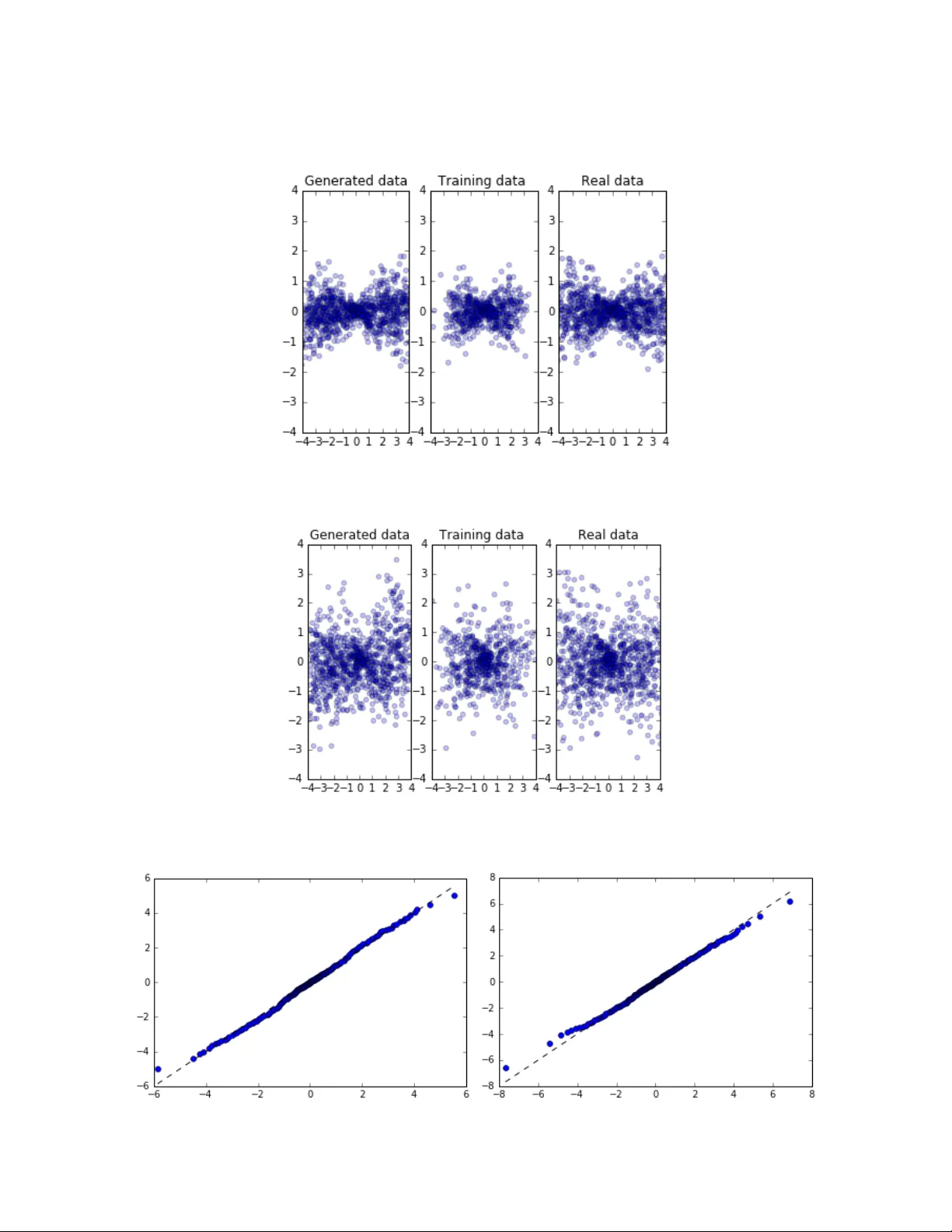
1 Time Series Sim ulation by Condit ional Gener ative Adver sarial Net Rao Fu 1 , Jie Chen, Shutian Zeng, Yiping Zhuang and Agus Sudjianto Corporate Model Risk Management at Wells Fargo Abstract Generative Adv ersarial Net (GAN ) has been proven to be a powerful m achine learning tool in imag e data analysis and gene ration [1]. I n this paper, we propose to use Condi tional Generati ve Adv ersarial Net (CGAN) [2] to lea rn and sim ulate time series data . The conditions can be both categorical an d continuous variables contain ing different k inds of auxiliary information. Our simulation stu dies show that CG AN is able to learn d ifferent kinds of no rmal and heav y tail distributio ns, as well as dep endent structur es of different tim e series and it can fur ther generate cond itional predic tive distribution s consistent with the training data distr ibutions. We also p rovide an in- depth discussion on the rationa le of GAN and the neur al network as hiera rchical splines to dr aw a clear connec tion with the existing stat istical method for distribution gene ration. I n practice, CGAN has a wide rang e of applications in th e mark et risk and counterparty risk analysis: it can be a pplied to lea rn the historical d ata and generate sce narios for the calculation of Valu e- at -Risk (VaR) and Expected Sho rtfall (ES) and p redict the m ovement of the m arket risk factors. We p resent a real dat a analysis including a back testing to demonstrat e CGAN is able to outperform the Historic Sim ulation, a popular m ethod in mark et r isk analysis fo r the calculat ion of VaR. CGAN can also be a pplied in the econom ic tim e series modeling and fo recasting, and an example of hypothetical shock analysis for economic m odels and the g eneration of potential CCA R scenarios by CG AN is giv en at the end of the pap er. Key words: Cond itional Generative Adv ersarial Net, N eural Network , Time Series , Market and Cred it Risk Managem ent. 1 Email: rao.fu@wellsfargo.co m 2 1. Introduction The modeling and g eneration of s tatistical distr ibutions, tim e series, and stochastic pro cesses are wide ly used by the financ ial institution s for the purposes of r isk manag ement, derivative secur ities pricing, and monetary policy making . For time series data, in order to capture the depen dent structures, Aut oregressive Model (AR), Gene ralized Autoreg ressive Condi tional Heteroscedas ticity (GARC H) Model, and their variants have be en introduced and int ensively studied in the literature s [3]. Moreo ver, as an alte rnative to the time series m odels, the stochas tic process m odels specify the m ean and variance to fo llow some latent stochastic proces s, such as Hull White model [4], Orns tein-Uhlenbeck proce ss [4], etc. Similarly , Copula, Copula-GA RCH model, and their var iants have been applied to captu re the com plex dependence structures in the generation of multivariate d istributions and tim e series [3]. However, all of the se models are strongly dependent on m odel assumptions and estim ation of the model param eters and, thus, are le ss effective in the estimation o r generation of non-G aussian, skewed, heavy- tailed distributions with time- varying dependent features [3]. Recently, GA N has been introduced and successfully applied in imag e dat a genera tion and learning . GAN is a generative m odel via an adv ersarial training process between g enerator network and discr iminator network, where bo th the genera tor and discrim inator are neural netwo rk m odels [1]. During the GA N training, the disc riminator train s the generator t o produce sam ples which resem ble real data from some random noise (u sually uniform or Gaussian variab les) and the disc ri minator is simultaneou sly trained to distinguish betw een real an d generated sam ples. Both neural n etworks aim to minimiz e their cost functions and stop on ce the Nash equ ilibrium is achi eved where none can continue improving [5]. Other variants of GA N have been introdu ced to improv e the training pro cess, such as Wa sserstein GAN (WGAN) [6], WGA N with gradien t penalty (WGAN-G P) [7], GAN with a g radient norm penalty (DRAGAN ) [8] [9], least s quare GAN (LSGA N) [10], etc. Alternat ively, instead of em ploying an unsupervised lea rning, Mirz a & Osindero [2] proposed a conditional v ersion of GA N, CGAN, to learn the conditional distrib utions. CGA N performs condition ing into both d iscriminator an d generator as an additional input layer [2] and g enerates conditiona l samples based on the pre-specified condi tions. In this paper, we p ropose to use CG AN to learn t he distributions a nd their dependent stru ctures of the time series da ta in a nonparam etric fashion and gene rate real-like conditional tim e series data. Specifically, C GAN conditions ca n be both categ orical and continuous v ariables, i.e., an indicator or historical data. Ou r simulation stu dy shows that: (1 ) Given categor ical conditions, C GAN is able to le arn different kinds o f normal and heavy tail distributions under different con ditions with a good perform ance comparable to the k ernel densi ty estimation m ethod, learn different correla tion, autocorrelatio n and volatility dy namics, and generate real-like conditional samples of t ime series data. (2) G iven continuous conditions, CGAN is able to learn the local changing dynamics of differen t time series and g enerate conditional predi ctive distributions cons istent with the original conditio nal distributions. 3 In term s of application, GAN and CG AN can be appe aling alterna tives to calculate Value- at -Risk 2 (VaR) and Expected Sho rtfall 3 (ES) for m arket risk m anagement [11]. Traditionally, H istorical Sim ulation (HS) and Monte Carlo ( MC) simulation m ethods have be en popularly used by major financial institutions to calculate VaR [11 ]. HS revalues a po rtfolio using actual shift siz es of mark et risk factors tak en from historical data, wh ereas MC revalues a portfolio by a large num ber of scenarios o f m arket risk factors, simulated from pre-built models. There are cons and pros in both m ethods. MC can produce near ly unlimited num bers of scenarios to g et a well-described dis tribution of PnL, but it is subject to large m odel risk of the stochas tic proces ses chosen. While HS includes all the correlations and v olatilities as embedded in the h istorical data, but the small num ber of actual his torical observations m ay lead to insufficiently def ined distribution t ails and VaR ou tput [11]. To overcom e these difficult ies, GAN, as a non-param etric method, can be app lied to learn th e correlation a nd volatility stru ctures of the his torical time series da ta and produce unl imited real-like sam ples to obtain a well- defined distribution. How ever, in reality, the co rrelation and v olatility dynam ics of historical data v ary over tim e, as demonstrated i n the large shifts expe rienced during the 20 08 financial cri sis. Thus, m ajor banks usually calculate VaR and Stressed VaR as the risk measu rements for norm al market periods and stressed period s (the 2008 financ ial crisis period). Thus, CGAN can be applied to learn historical data and its dependen t structures unde r different m arket conditions non- parametrically, and pro duce real-like condition al sam ples. The conditional sam ples can be g enerated unlimitedly by CGAN and used as scenarios to calculate VaR and ES as the MC m ethod. GAN and CGA N can also be app lied to econom ic forecasting and m odeling, whic h has several advantages over traditional econom ic models. Traditio nal economic m odels, such as Macro A dvisers US Model (MAUS) 4 , can only produce a s ingle foreca st for giv en a condition and under strong m odel assumptions. By contrast, GA N can be applied as an assumption – free m odel to produce a forec ast distribution given th e same sing le condition. The g eneration of the forecast distrib utions can be a us eful source of scenarios for Com prehensive Capital Ana lysis and Review (CCA R) for financial institutions [12]. In Sect ion 2, we form ally introduce the GAN , WGAN, D RAGAN, and CG AN, and the prop osed an algorithm for CG AN training . We, then, prov ide an in-depth discussion on the neural netw ork models as hierarchical sp lines and the rat ionale of GAN to learn a distr ibution in Section 3 . The simula tion studies of CGAN with d ifferent distr ibutions, tim e series and dependent structures are pro vided in Section 4 . We 2 VaR is the most i mportant measurement in market ri sk manage ment, which is the assess ment of the potential los s of a portfolio over a given time period and for a given distribution of historical Pro fit -and -Loss (PnL).VAR can b e calculated for a pre -specified perce ntage probability of loss over a pre -specified period of time. For example, a 10 - day 99% VaR is the do llar or percentage loss in 10 days that will be equaled or exceeded o nly 1% of the time (usually over 252 business days or 1 year). In other words , there is a 1% pr obability that the loss in po rtfolio value will be equal to or larger than the VaR measure ment [11]. 3 ES is another po pular measurement o f risk in market risk m anagement, as it satisfie s all the prop erties of coherent risk measurement, includi ng subadditivity. Mathe matically, ES is the expec ted loss given the po rtfolio return alread y lies below the VaR. T hus, ES gives an esti mate of the magnitude of the los s for unfavorable events, but VaR only provide a lower limit o f the loss. ES is going to b e implemented in the internal models approach (IMA) under the Fundamental revie w of the trading book (FRTB) framework in around 3 years by major financial institutes [1 1][13] . 4 The MAUS model i s used to generate multiple US macroeco nomic forecasts for various a pplications b y financial institutes. More details ca n be found at www.macroadviser s.com. 4 also present two real data studies in S ection 5, whi ch includes a backtesti ng for mark et risk analysis to demonstrate tha t CGAN is able to ou tperform the HS m ethod for the calculation of VaR and ES. We al so provide an exam ple of a hypothe tical shock analy sis of econom ic models and the generation of po tential CCAR scenarios. Section 6 covers further di scussion and potent ial improvem ent. 2. GAN & its Variants 2.1 GAN GAN training is a minm ax game on a cost function between generato r (  ) and discriminator (  ) [1], where both  and  ar e neutral network m odels. The input of  is  , which is usually sampled from a uniform or Gauss ian distribution. Form ally, the co st objective fu nction of GAN is:         󰇟  󰇛󰇜󰇠      󰇟  󰇛   󰇛   󰇜 󰇜󰇠󰇛󰇜 where   is the real data distribution and   is the model dis tribution im plicitly defined by     󰇛  󰇜 . Both  and  are trained simul taneously, whe re  receives either gene rated sam ple   or real data  , and  is trained to distinguish the m by m aximizing the cost function. While,  is trained to g enerate more and more realistic sam ples by m inimizing the cost f unction. The tra ining stops when  and  achieve the Nash equilibrium , where none of them can be fu rther im proved through training . In the original p aper of GAN [1], the authors also p roposed to upda te the cost function by maxim izing the probability of generated sam ples being real, instead of minim izing the probabili ty of being fake i n practice. Howev er, Google Brain cond ucted a larg e-scale study com paring these methods, but they did not find any significant dif ference in perform ance [14]. Thus, we applied 󰇛󰇜 as the origina l GAN m ethod. 2.2 WGAN & DRAGAN One of the main f ailure modes f or GAN is the g enerator to collap se to a param eter setting where it alway s generates a sm all range of outpu ts [6]. The literature s uggests that a local eq uilibrium in this minmax game causes the m ode collapse i ssue [8]. Another m ajor issue is the dim inished gradient: the discriminator get s too successful that the generator gra dients vanish and the generator le arns nothing [6]. Two alternativ e GANs have been in troduced to solv e these training issues. On the one hand, WGA N utilizes a new cost function using Wasserst ein distance, w hich enables the generator to im prove in any case as the Wasser stein distance be tween two distribut ions is a continuous function and diffe rentiable alm ost everywhere. Th e cost function of WGAN simpli fied by Kantorov ich - Rubinstein dual ity is:          󰇟  󰇛󰇜󰇠      󰇟  󰇛   󰇜 󰇠 󰇛󰇜 where  is the collection of a ll 1-Lipschitz funct ions. The literatur e suggests that th e gradient of th e discriminator of WGA N behaves bet ter than GAN’s rendering the opt imization of the generator eas ier [6]. The Lipchitz conditions are en forced by weight c lipping by a sm all value in the or iginal WGAN 5 paper. Later, Gulr ajani et al. [7] proposed to add a gradien t penalty in the co st function of WGA N to achieve the sam e condition ins tead of using the weig ht clipping m ethod. However, according to th e large - scale study by Google Brain [14] there is no strong evi dence showing that WGAN-GP consisten tly outperform s WGAN after sufficient hyper-parameter tuning and r andom restarts [14]. On the other hand, D RAGAN is propose d to solve the same issues throug h a gradient penal ty directly to GAN. The authors o bserved that the l ocal equilibri a within 󰇛󰇜 often exhibit shar p gradients of t he discriminator arou nd some real da ta points and dem onstrated that these degenerate d local equilibr ia can be avoided with a g radient penal ty on the cost function. Form ally, the cost funct ion of DRAGA N is:     󰇝󰇛󰇜       󰇛  󰇜 󰇟 󰇛  󰇛   󰇜   󰇜  󰇠󰇞  󰇛󰇜 Kodali et al. [8] showe d that DRA GAN enables fast er training w ith fewer model c ollapses and ach ieves generators with better perform ance across a variety of architecture s and objective functions. 2.3 CGAN A conditional v ersion of GAN is in troduced by Mirz a & Osindero in 2014 [2], wh ich enables GAN to generate specifi c samples g iven the conditions. CGAN conditions take any kind of auxiliary information from the sam ples and gives a head start to the g enerator to create sam ples. The sam e auxiliary condition, usually denoted by  , are applied to both g enerator and d iscriminator as add itional input layers. The original input noi se variable  is combined with  in joint hidden repres entation [2] . Form ally, the cost function 5 for CGAN is:         󰇟  󰇛 󰇜󰇠     󰇟  󰇛   󰇛  󰇛 󰇜 󰇜 󰇜󰇠󰇛󰇜 where   is the distribu tion of the random noise, which is usually uniform or Gaussian as the GA N. Similarly, it is e asy to make a con ditional WGAN (CWGAN) by passing the con ditions to the cos t function:          󰇟  󰇛 󰇜󰇠        󰇛   󰇜  󰇛󰇜 CGAN w ill be degenerated to G AN giv en a single categ orical condition and training CGAN w ith multiple ordina l categorical condi tions is not equiv alent to train ing multiple GAN s on each of the conditions, where the former is m uch harder than the latter in the term of the learning difficul ty. It is because the traine d CGAN only contains one se t of weights/paramete rs, but able to ad just and generate different distribu tions given different condition s. On the other hand, CG AN is able to leverage the relationship am ong different ca tegorical condition s, and effectively utilize the data information acr oss different categ orical conditions. Another difference is CGAN can be tra ined on continuous conditions, which is beyond the reach of using multiple GAN s. 5          󰇟󰇠           󰇟  󰇛󰇜󰇠    󰇟󰇛   󰇛  󰇛󰇜 󰇜 󰇜󰇠 , which is essentiall y the same as (4) in practice. 6 The CGAN describe d in equation (4) is our main m ethodology in this paper, and will be tested in the simulation stud ies under the differen t conditions desc ribed in Sect ion 4. An algori thm for CGAN training is also developed w ith the considera tion of all the m ajor numerical difficul ties in the existing literatures. For exam ple, we observed that the m ode collapse rem ains a major issue in CGAN and we currently applied a weight clipping ad justment to remov e the sharp gradients o f the discrim inator, which is in the sam e spirt of WGAN and DR AGAN to add som e gradient penalty on the discrim inator. We also fou nd that the alg orithm performs better w ithout batch norm alization after adding the gra dient penalty, w hich is similar to the sug gestion giv en by Gulrajani et al [7]. We us e Adam as the opt imization com puter as it is the most popular ch oice in the GA N literature [14]. Th e neural network s for both discrim inator and generator are c onstructed b y fully connected l ayers followed by Leak yRelu 6 activation funct ions and implem ented in Python Keras Py thon Deep Learning library [15]. In summ ary, the algorithm of the CGAN is: Algorithm of CG AN :   is the number of discrim inator iterat ions per generator iteration.  t he hyper- parameter for weig ht clippi ng. for number of tra ining iterations do for   steps do  Sample a batch from the real data  and their correspon ding conditions  .  Sample a batch o f noise  from   .  Passing  ,  ,  to the cost function ( 󰇛  󰇜 for CGAN, 󰇛  󰇜 for CWGAN) and upd ate the discriminator by as cending its sto chastic gradien t using Adam .  Weight clipping (  ,  ) to discriminator. end for  Sample a batch o f noise  from   .  Update the genera tor by ascending its stochastic g radient using Adam. end for 6 Leaky Rectified Linear Uni t function (LeakyRelu) with  :  󰇛    󰇜           . LeakyRelu attempts to fix the “Dying ReLU” pro blem, where a large grad ient flowing through a ReLU neuron could cause the weights to update in such a way that the ne uron will never activate o n any data point again. 7 3. Rationale of GAN A single layer neu ral network is a non-linear transform ation from its input to its outpu t. A deep neural network can be v iewed as a composition o f several inte rmediate single layer neural netwo rks. It is easy to show that a sing le-layer forward neu ral network with a ReLU 7 activation funct ion is a m ultivariate affine spline (also know n as piecew ise linear spline) [16] and , thus, a deep forwa rd network can be w ritten as a hierarchical mult ivariate affine s plines. Actually , there is a rigorou s bridge betwee n the neural netwo rk models and the a pproximation the ory via spline fun ctions, and a l arge class of dee p networks m odels can be written as a com position of m ax-affine spline func tions [17]. In this paper, w e work exclusiv ely with network m odels with forward connec ted layers fo llowed by ReLU ty pes of activation fun ctions, but the ideas can be gene ralized naturally to the other ty pes of layers and a ctivation funct ions. Let’ s first focu s on the rationale of the simulation of un ivariate distribu tions by GAN. In order to g enerate a real-like distr ibution, the g enerator of GAN, a neura l network model, is essential ly trained by the discriminator to learn the em pirical inverse CDF of th e training data by spline functions and operators in a non- param etric fashion. For exam ple, let’s train a GAN w ith the  containing a sin gle fully connected layer with 7 nodes followed by a ReLU activ ation function, and  is constructed similarly. The input of  ,  , followed a U(0, 1) dis tribution, and th e training dat a,  , followed a N(0, 1) dist ribution. Theoretically, the number of k nots of the spline sp ecified by a single layer netwo rk is bounded by the number of the network nodes [16]. I n this example, the netwo rk,   is trained to result in a piecew ise linear spline fun ction with 2 spline k nots within [0, 1] (the m eaningful dom ain of this m apping) after 10,000 iterations o f training, and the o ther 5 knots are e ither overlapped a t the ones plotted in F igure 1(left) or located ou t of [0, 1]. I t is worth to point out that, here, the tra ining data  is total ly independent with  input   , and the network m odel cannot be trained by a sim ple loss funct ion (such as the mean squared error o r entropy) for a com mon supervised lear ning problem [15]. GAN , as an unsuperv ised leaning m ethod, provide a non- trivial alternative to learn the same m apping to m atch the inverse CDF of N(0, 1) from sam ples random ly sampled from U (0,1) , which is due to the help f rom the  t rained simultaneously with  . Next, in order to o btain a sm oother spline approxim ation, we increased th e node num ber of  fr om 7 to 100 for this exam ple. Batch size and training iterat ions are increased as we ll. The result are provided in Figure 1(right), in w hich the location a nd number of the spl ine knots are ref ined to result in a smoother spline approxim ation to match the targ et function. And sim ilarly, most of the splin e knots are overlapp ed at the ones plotted in Figure 1(right) or located out of the support [0, 1]. Th ere is no ov erfitting in this particular exam ple, and this is expec ted, as the CDF f unction of N(0,1 ) is a monot onic and smooth target function and it shou ld be fitted by a sim ple spline appr oximation. In the previous exam ples, we dem onstrated that GAN w ith a  cont aining more nodes of a sing le layer network results in a smoother sp line approxim ation. Next, we s how that using a  containing deeper layers results in a sm oother appro ximation as well. For example, we t rained a GAN w ith the same parameters as the pr evious exam ple, except that the  containing two ful ly connected layers w ith 100 nodes on each lay er followed by R eLU. The result is d epicted in Figure 2 (le ft), where a sm oother spline approximation is obtained. H ere, the usage of network s with multiple lay ers with ReLU func tions is 7 Rectified Linear Unit fu nction (ReLU):  󰇛  󰇜   󰇛  󰇜 8 essentially to const ruct a non- linear mapping by hierarc hical spline s. Thus, the smoothne ss of this approximation is expected. Figure 1 Left: 1-layer with 7 nodes; Right: 1-layer with 100 nodes. Blue line: inverse CDF from U(0,1) (x-axis) to N(0, 1) (y -axis), Green line: spline approximation trained by GAN. Figure 2 left: 2-layer with 100*100 nodes with 1 input variable. Right: 1 -layer with 100 nodes with 3 input variables Blue line: inverse CDF from U(0,1) (x-axis) to N(0, 1) (y -axis), Green line: spline approximation trained by GAN. Furthermore, instead of using a single random v ariable as the input fo r  ,   can be sourced from multiple random v ariables. For exam ple, suppose we decid e to learn an univar iate N(0, 1) by GAN with 3 independent unif ormly distributed r andom v ariables as the inputs to  , then this is essentia lly training a   to  spline to m ap appropria tely from the noise spac e to the simulated sam ple space. The in clusion of the multiple inputs to  can also encourage sm oothness. For example, we retr ained GAN with  containing 1 lay er with 100 nodes, but the inputs became 3 independ ent uniforml y distributed random variables. The r esult is depicted in Fig ure 2 (right), where we plotted the em pirical CD F of the output samples of  , which perfectl y matched the CDF of the N(0,1). In term s of the generation of m ultivariate distribut ions, the classical method, Copu la, usually constru cts a complicated m apping from independen t uniform variates to the outcom es and depends on strong m odel assumptions of di stributions and p arameters to ca pture the correlat ion structures. However, GA N provides a straightforward, non- param etric and unsupervised a lternative to bu ild the non-linear m apping through 9 neural networks. I n section 4, we wil l present sim ulation studies to show G AN type m ethod is able to capture the key features of dis tributions and cor relation structures of different m ultivariate dis tributions and time series. In summ ary, both  and  of GAN, as neural netwo rk models, can be wr itten as a c omposition of spl ine operators. A sm oother spline app roximation can be o btained using deep layers, lar ge num ber of no des, and multiple rand om variables as inpu ts to  . CGAN builds non-linear m apping from inputs to outputs with the sam e rationale as GA N. Howev er, the key difference betw een CGAN an d GAN is that CGAN uses additional v ariables, which are the condition s given by the user. Th e condition v ariables are not independent from the training data. Thus, CGAN is a semi-supervised learning m ethod. 4. Simulation Study In this section, we d emonstrate that the performance o f the CGAN m ethod on: (1) Mixture of Gaussian distributions wi th various m eans and variances, inclu ding an example o f extrapo lation by CGAN. (2) Vector autoreg ressive (VAR) tim e series with heav y-tail underling noise and region switching features. The usage of heav y-tail distribu tions simulates the be havior of re al financial da ta. The region swi tching time series is a t ime series with d ifferent dependent structu res from diffe rent time periods /regions, and it is used to sim ulate the real m arket mov ements occasionally exhib iting dramatic br eaks in their behav ior, which are associa ted with ev ents such as financia l crises. (3) Mu ltivariate generalized au toregressive conditional heterosc edasticity (G ARCH) time series w ith heavy- tail underling noise. Note that bo th VAR and GARCH m odels are usually used as param etric models in the financ ial time series a nalysis, such as the modeling and prediction of stock rerun, GDP, etc. We show that CGA N, as a nonpar ametric m ethod, can learn dependen ce struct ures of these tim e series and sim ulate conditional predictive tim e series. To assess the est imation of the h eavy tail distribu tions by CGAN, we use one of the most classic non- parametric m ethods, Gaussian k ernel density estim ation, as the benchm arking m odel, where a cross validation method is used to find th e best tuning parameters for the k ernel estim ation. The estim ation is implem ented in python scikit learning library [18]. In term s of the architectures of  and  of CGAN, w e use a 3-layer forward co nnected network with 100+ nodes for each layer followed by Leaky Relu (    ) activation func tion for both  and  . The inputs of  are 30 random variables. In this m aner, we allow CGAN to have enough com plexity and capacity to learn different kinds o f multivariate distribu tions and tim e series. According to the Goog le Brain large- scale studies [14], m ost GAN m odels can reach sim ilar performance with enough hyper- parameter optim ization and random restarts. Thus, we work with CGAN in the fol lowing sub-section, where the hyper- parameters are set or trained in th e similar setting as the large-scale study from Google Brain [14]. CWGAN is also tested w ith several exam ples and resu lts are comparable with CGAN ’s . 10 4.1 CGAN for Gaussian Mixture Model We first dem onstrate different u ses of CGAN to learn and genera te a Gaussian m ixture distributions. Similar sim ulation tests have been conducted on T-m ixture distributions, and the results are comparable and can be made av ailable upon r equest. 4.1.1 Gaussian Mixture Model with nominal categorical conditions The CGAN m ethod is first tested on a m ixture of Gaus sian distributions with var ious means and variances. Four c lusters of 2- dimensional Gaussian di stributions (i.e., the training data     ) with various means and v ariance are gene rated (see Figure 3, right p anel), where the sample size for eac h cluster (label led by different color s) is 1000. The cluste r numbers (0, 1, 2, and 3 ) are the nom inal categorical condi tions, which ar e transform ed into dumm y variables and used in the CGAN training . Thus, the current inputs to  are  and  , where  is the random noise and  is the dummy variable categorized for t he clusters. I n order to learn and s imulate the sam ples for each condition, the CGA N actually trains fou r non-linear m appings simultaneousl y, and each non-linear m apping would be applied to generate the sam ples for each clu ster by setting the condition  properly. In this simulation, CG AN is trained wi th 10000 itera tions and used to gene rate the four clusters wi th the same sam ple size (see Figure 3 left pane l). QQ-plots 8 are given to com pare the generated d istributions and the original ones respectively , and the results show a g ood match to eac h other. The benchm arking method, Gauss ian kernel estim ation, is applied to ea ch cluster, and the generated d ata by kerne l method is compared to the re al data. The ben chmarking results (Figure 4) show that CGA N and kernel densi ty estimation m ethod have com parable model perform ance in this exam ple Figure 3 2-dimensional Gaussian Mixture distributions: CGAN generated data (left) vs. real data (right). X-a xis is for dimension 1 and y-axis is for dimension 2. 8 The QQ-plots are comparing the 1 st dimension of the ge nerated distributions and the or iginal ones (also ap plied to all the QQ-plots in the following context). T he results of the co mparison of the 2 nd dimension are co mparable. 11 Figure 4 Left: QQ-plot comparing real data vs. CGAN generated data for cluster 1. Right: QQ-plot comparing real data vs. by Kernel estimation generated data for cluster 1. (The results for the other clusters are comparable.) 4.1.2 Gaussian Mixture Model with ordinal categorical (integer) c onditions In the previous sub- section, the condi tions work as the labels of the c lusters and a re transferred in to a dummy variable before passing into the CGAN training process. Altern atively, we can p ass the label numbers (0, 1, 2 and 3) directly in to CGAN. Thus, the inputs to  are  and  , where  is an integer variable. Howev er, there is no uniq ue labelling of the conditions by integ ers, and we find that a comparable scale s between the data and integer condi tions usually g ive efficient and robu st results based on our experim ents. Therefore, we recom mend rescaling both the training and conditioning data sets properly before the GAN learning process, or always u sing dummy variables as inputs to nominal categorical condi tions. However, an adv antage of using in teger conditions is extrapolation. Spec ifically, w e can train a CGA N with integer cond ition  and feed decimal con dition valu es into the CGAN w hen generating the conditional sam ples. For exam ple, we use CGAN to learn the cluste rs in Figure 3 (right panel), and generate the orig inal clusters and extrapo late the expect ed clusters between the origina l clusters (Figure 5, left panel), where the extrapolated clusters located pro perly between the original c lusters with reasonab le shapes. Especial ly, the clus ter in Figure 5 (right pan el) has a mixed shape between the o riginal cluste rs. This implies tha t the trained  of CGAN provides a no nlinear mapping from noise space to simulated sample space that con tains a continu ous information about the locat ion, shape, mean, v ariance, and other statistics to gene rate and extrapolate cond itional sam ples for different clu sters. 12 Figure 5: Examples of the extrapolation clusters from the original 4 clusters 4.1.3 Gaussian Mixture Model with Continuous Conditions Next, we assum e each data poin t of the training data set is sampled from hom ogeneous distribution s with key features v arying sm oothly. Therefore, in order to c apture the varying features, we use CGAN w ith continuous condi tions. Again, as we discu ssed in 4.1.2, both the data and the conditions woul d be rescaled if their o riginal sca les are not com parable. In the following sub- section, we will first assess the CGAN training and generation on continuous conditio ns and then ass ess the extrapolation properties using CGAN by setting the cont inuous conditions acco rdingly. First ly , the t raining data for CGAN is generated by G aussian distribut ions with vary ing means and variances for each data point: (1) Generate the m eans, which a re 1000 separated points along the circle with center at (0, 0) and radius =  . The m eans are going to be used as the continuo us conditions in CGAN training . (2) Generate 100 0 variances co rresponding to each m ean, which are linearly increa sing along the circle in an anticlock wise direction. (3) The final data is g enerated by Gaussian d istribution with its mean along the circle an d its corresponding variance (Figure 6 ). CGAN is trained t o learn this synth etic distribution, g iven the 1000 m eans as continuou s conditions in the training. The out puts are disclo sed in Figure 6, and a Q Q-plot is drawn to compare the gener ated distribution with the original on e. The results c learly im ply that CGAN successfu lly learns the dy namics in the data and is able to genera te real-like sam ples. Secondly, sim ilar to the CGA N with integer conditions, one o f the most im portant advantage of CG AN with continuous con ditions is extr apolation. In the first exam ple, the dynam ics of the chang ing of variance are indi rectly passed in to CGAN from the continuous conditions (their means). Thus, we can use CGAN to extrapo late samples bey ond the original sup port, if we feed the CGAN the c onditions beyond the original suppor t. 13 Figure 6 left: CGAN generated data vs. real data. Right: QQ-plot: comparing real data vs. CGAN generated data. We conduct anothe r simulation study to assess the ex trapolation prope rty by CGAN w ith continuous condition. The train ing data is g enerated following the procedur e in the previou s example except the variance is chang ing along the x-axis bu t not a circle. In Fig ure 7 (right panel), th e entire 1000 training data was generate d according ly, where the variance of each data point increases from the original point to both directions a long the x-axis. N ext, the first and l ast 20% of the 1000 da ta were clipped d uring the CGAN training and CGAN is trained on the rem aining 60% data with th eir corresponding 60% m eans as conditions (Figure 7 , middle panel). After the CGAN training, we s imulate and extrapola te 1000 sam ples with the origin al 1000 means as continuous conditions . Note that the f irst and last 20% of the g enerated data are not within the support of the o riginal train ing data, but extrapo lated by CGA N ( Figure 7, left panel). Again, QQ- plots are created to compare the com plete distribution g enerated by C GAN and the original whole d istribution (Figure 9 left panel). The re sults clearly evidence that CGA N demonstrates a good perform ance of extrapolation at the tails of th e distribution, wh ere CGAN learns the dynam ic in the changing of the v ariance is furthe r able to extrapolat e the samples bey ond the original supp ort following the same dy namics. Furthermore, we c onduct a similar sim ulation, where t he variance increa ses along the x-axis from the original point w ith a faster speed. The results (Figure 8 and Figure 9 right pan el) show that CG AN can learn different m agnitudes of the ch ange dynam ics and produce real- like conditional distribut ions. This is very important i n terms of prac tice as we usually ca n only access the tre nd of the chang e dynam ics, but not the mag nitude and mechanism . Using CGAN, w e can learn the chang ing dynam ics on the support of the training data w ithout any parametric assum ption and further extr apolate the dat a to the unknow n area with the sam e dynamics learned from the train ing data. 14 Figure 7 Slow Variance increasing Scenario – Left: 1000 samples generated by CGAN with the original 1000 means as continuous conditions, middle: clipped data used in the CGAN training. Right: the original 1000 samples. Figure 8 Quick Variance increasing Scenario: left: 1000 samples generated by CGAN with the ori ginal 1000 means as continuous conditions, middle: clipped data used in the CGAN training, right: the original 1000 samples. Figure 9 QQ -plot comparing the generated data vs. real data. Left panel: Slow Variance increasing Scenario, and right panel: fast Variance increasing Scenario: 15 4.2 CGAN for VAR Time Series In the following sub-sections, we extend the usage of CGAN to the lea rning and g eneration of time series data. Financial tim e series analy sis is a highly em pirical discipline, and numerous classic stat istical models have been d eveloped and em ployed in applicat ion, such as AR, A RMA, ARC H, and GARCH [3][1]. In order to have a com plete view of the CGAN i n time series data m odeling, we condu ct simulation stud ies on AR and G ARCH-type tim e series, where the form er usually has a strong autocorrelation and t he latter has a s trong volatility dynamic. VAR m odel generaliz es the univariate AR model, and applied to capture the line ar dependent s tructures am ong multiple time series. The notation VAR (  ) indicates a v ector autoreg ressive m odel of order  . Mathematically, the m odel can be def ined as:                󰇛󰇜 where 󰇝       󰇞 ar e the autoco rrelation param eters,  is a constan t and   is an underly ing noise. I n this sub-section, we g enerate 󰇝                󰇞 a 2 -dim ensional VAR (1) tim e series, as the training data for CGAN m odeling. The underlying noises of   are sampled from a T distr ibution, which simulates the he avy tail dist ributions usually obse rved in the fin ancial tim e series. Fur thermore, we d efine the following term inologies as the main statis tics to assess the 1 st order correlat ions: 1-lag autocorrelation for tim e series       󰇛    󰇜  󰇛  󰇜󰇛  󰇜 , correlation betwee n time series  and       󰇛    󰇜  󰇛  󰇜󰇛  󰇜 , cross correlatio n between tim e series and time lag s      󰇛     󰇜  󰇛  󰇜󰇛  󰇜 . Next, we define the 2 nd order 1-lag autoco rrelation as:     󰇛      󰇜  󰇛   󰇜󰇛   󰇜 .   , is used to asse ss the volatility dy namic of the GA RCH time series, whe re the 2 nd order autocorrela tion is usually larg er than the 1 st order. The 2 nd order correlation be tween tim e series (   ) and cross corre lation (   ) can be defined similarly . The following sub-section is separated into three parts: 4.2.1 CGAN m odeling with continuous conditions, 4.2.2 CG AN modeling with continuous co nditions for region switchin g time series, and 4.2.3 CGAN m odeling with categ orical conditions fo r region switchi ng time series. 4.2.1 CGAN Modeling with Continuous Conditions We assume the training data alway s follows a sim ple VAR (1) proces s with the f ollowing parameters:           , (7) 16   󰇟 󰇠  ,   󰇟 󰇠  ,   󰇛      󰇣     󰇤    󰇜 , Note that the unde rlying noise v ariable,    follows a T- distribution with a d egree of freedom of 6, which has a much long er tail than a standa rd norm al di stributi on. The VAR m odel specifies that the outp ut variables linea rly depend on the ir own previous v alues and on random noises, thu s we propose using the previous 1- time-lag values of th e time series as the conditions for the CG AN m odeling of the current tim e series values. Th e CGAN should b e able to capture the dependent st ructure of VAR (1), and mak e 1 -time- horizon predic tion by giv en the current value as the c ondition. By this setting, the data form at of both the tra ining data and condition data is: Sample siz e x Number of Tim e Series (TS) = 1 ,000 x 2  where the condition data set is constru cted by taking 1-tim e-lag sliding-w indow snapshot of the training data. We begin by asses sing if the CGA N outputs are truly conditional on their 1-tim e-lag conditions. Suppo se there are two ad jacent AR ( 󰇜 tim e series outputs    and   , and the 1-lag autocorrelation between   and   is  . If the CGAN is able to learn the dep endent struc ture of VAR ( 󰇜 , then the 1- lag autocorrelation b etween    and   , generated by C GAN given   and   respectively, shou ld be   mathem atically. Similarly, the 2-lag autocorrelation betw een   and   should be   . During the CGAN training , we track b oth the autocorrelations be tween    and   during each it eration, which ar e the blue (for 1- lag) and green (for 2- lag) lines presen ted in Figure 10. The ho rizontal straig ht lines in Figure 10 repres ent the correspond ing theoretical v alues of these statistics, w hich are   for 1-lag and    for 2-lag. Fig ure 10 shows that the autocorrelation s from the CGAN generated da ta converge to their theoretical valu es, however the m ovement of these s tatistics is relatively v olatile. This is becau se the sample size of the t raining data is small, and it ca n be im proved by the increase of sample size (see an example in Fig ure 16). In summ ary, the result shows t hat CGAN is able to le arn the autocorre lation and generate a tim e series with an exp ected dependent stru cture. In 4.2.3, we in troduce an altern ative to generate a tim e series containing the or iginal dependent struc ture by using CGAN with categoric al conditions. Figure 10 Tracking results of autocorrelation (blue c urves for 1 -lag, green curves for 2-lag) over 10,000 CGAN learning iterations for time series 1 and 2. The horizontal straight lines are the corresponding theoretical values of these statistics. 17 We then assess the 1-time-horizon pred iction made by C GAN. The CGAN will b e firstly trained g iven the 1-time- lag values as conditions, and then a conditional d istribution g iven a single cond ition will be generated by CG AN and com pared with the true condi tional distribution spec ified by equation (7 ). The true conditional d istribution is def ined through the condition values (   ), autocorrelation pa rameters of VAR(1) (  ) and the underlying noise distribution (   ). In the prev ious section, we already demonstrated that CGAN is ab le to capture t he autocorrelat ion. Therefore, in order to further test if CG AN can capture the underlying noise distribution and its dy namic, we let the v ariance of the dis tribution of   vary with the sum of the abso lute value of 1- time-lag tim e series values. Form ally, the traini ng data is generated by:         , (8)   󰇟 󰇠     󰇛      󰇛     󰇜   󰇣     󰇤  DF   󰇜 . Here, CGAN was f irstly trained w ith 10,000 iterations, where the training and co ndition data format is still: Sample size x N umber of TS = 1,000 x 2. After th e training, 500 co nditional 1- time-horizon distributions g iven 500 random selected conditi ons were generated and compared w ith the true one s. The sample size of ea ch generated dist ribution is the sam e as 10,000. The distribu tion com parison is conducted in two w ay: (a) QQ - plot: For each condi tion, we draw a QQ- plot to compare the sim ulated conditiona l distribution and the true condi tion distribution. And we fit a linear regr ession to assess the f it of the QQ-plot, whe re the R square and the sl ope for each com parison are saved and plotted as a histogram plot in Figure 11. There is a clustering at 1 on x-axis for both R squ ares and slope s, which indicates a good m atch. (b) We com pare key statistics (mean, v ariance, skewne ss, and kurtosis) betw een the 500 gener ated conditional distrib utions by CG AN and the correspond ing true condition al distributions. These statistics are plotted in Fig ure 12 as scat ter plots. For exam ple, the means and v ariances vary in this simulation, and their values from the true condi tional distribu tions (x-axis in Figure 12) are m atched along 45 deg ree line with the ones from the generated co nditional distribu tions by C GAN (y-axis in Figure 12), which implies that CGAN is ab le to capture t hese local changes giv en the conditions. The skewness and kurtosis are fixed in this sim ulation, which expl ains why they are located along a vertical line, and the intersection of this vertical line and the x-axis is the ir true values. The skewness from CGAN is distribu ted around the true value 0 with a reasonable range of variation com pared to the range of the data . T he excess kurtosis should be 0 for th e normal distribution. Bu t, here, the kurtosis value shou ld be larg er than 0 as the underlying noise has a T-distributio n with degree f reedom of 20. How ever, there are a few c ases where the kurtosis is low er than 0, indica ting an underes timation of the heav y-tails, which is unexpecte d and may not lead to we ll described tai ls. The underestim ation of the heav y-tails is due to the ins ufficient sample s ize of the training data. Another simulation study was conducted w ith a much larg er sample: Sample size x Num ber of TS = 20,000 x 2 . The new results (F igure 13 , Figure 14) show that the 1- time- horizon predication is im proved, where the mom ents from the conditional dis tributions are all close to the the ir true values including the k urtosis estimated suff iciently to reflect the he avy-tails. Thus, we conclude that CGAN training is af fected by the sample size of th e training data, especially for capturing the higher order moments of the d istribution. 18 Figure 11 histogram of slope (1 st column) and R square (2 nd column) of the QQ plots comparing distributions generated by CGAN vs. VAR( 󰇜 . 1 st row for the 1 st time series (TS), and 2 nd row for the 2 nd TS. Figure 12 Mean (1st), variance (2 nd ), skewness (3rd) and kurtosis ( 4th) between the CGAN generated samples (y-axis) and real VAR(1) generated samples (x-axis). 19 Figure 13 Larger sample size: histogram of slope (1 st column) and R square (2 nd column) of the QQ plots comparing distributions generated by CGAN vs. VAR( 󰇜 . 1st row for the 1 st time series (TS), and 2 nd row for the 2 nd TS. Figure 14 Larger sample size: Mean (1 st ), variance (2 nd ), skewness (3rd) and kurtosis (4th) between the CGAN generated samples (y-axis) and real VAR(1) generated samples (x-axis). Similarly, w e test VAR (1) time series with oth er volatility changing dy namics, such as:          (9)   󰇟 󰇠      󰇡           󰇣     󰇤     󰇢  The results are com parable, and indic ate the CGAN is able to capture different kin ds of dynamics of th e underlying noise. In summary, w e concluded that CG AN is able to lear n the depe ndent structure of the VAR tim e series and the heav y tails of the underly ing noise. CGAN can furt her generate the conditional 1-time-horizon pred ictive distribut ions with the sam e key statis tics as the training data giv en enough sample sizes. 20 4.2.2 CGAN modeling with continuous conditions for region switching time series The region switch ing time seri es is a time serie s with differen t dependent struc tures from different tim e periods. As we dem onstrated in Se ction 5 .1 , both the autocorrelation pa rameters and the k urtosis of the time series da ta of equity returns exhib it large changes from the financial cr isis period to the norm al period. In order to s imulate thi s behavior, we further a ssume that the tim e series of the train ing data follows two diff erent VAR(1) proces ses in diffe rent periods in this sim ulation. Specifically, the f ormat of the training data is: Sample size x Num ber of TS = 20 ,000 x 2,where the firs t 10,000 x 2 samples a re generated giv en the param eters in region 1, and the re st are generated using the param eters in region 2. Note that region 1 and 2 have differen t VAR param eters for autocor relation and under lying noises given below: Region 1:            󰇛  󰇜   󰇟 󰇠  ,   󰇟 󰇠  ,    󰇡      󰇣     󰇤    󰇢 Region 2:   󰇟 󰇠  ,   󰇟 󰇠  ,    󰇡 󰇣     󰇤   󰇢 In this simulation, w e follow the sam e strategy used in section 4.2.1 in which the prev ious 1-tim e-lag time series values are the conditions for CG AN training. How ever, the goal is to test if CG AN can identify the region switch effec t: the chang es in the VAR paramete rs for autocorrelat ion and underly ing noises. CGAN is trained wi th 10,000 iterations, and the region switchi ng effect is ass essed by a comparison of key statistics by sca tter plots as sec tion 4.2.1. However , here, 500 conditions are random ly selected from region 1, and produc t Figure 15 (left pane l); and an oth er 500 conditions are sam pled to plo t Figure 15 (right panel) for reg ion 2. The plots show that the reg ion switching effect is captured by CGA N, because (1) the change of the VAR param eters are captured, as the m eans from the gener ated distributions and the true distributions are matched for bo th regions. (2) The chang e of variance an d the degree of f reedom of the underlying T distribution are captur ed. For exam ple, the excess kurtosis from region 1 is concen trated at 2, while the one from region 2 is conce ntrated at 0.7 5. This result is expected si nce the degree o f freedom of the unde rlying T distr ibution for region 1 is 6, resu lting in a heav ier tail of the distribut ion compared to the one u sed in region 2 (degree of freed om is 12). In conclusion, th e result implies that CGAN is able to capture the reg ion switch in g effect in this exam ple. Here, region 1 and 2 a re generally not overlapped (see Figure 17, up- right), thus continuous cond itions are sufficient. Fo r more general r egime switching cases where there are a larg e amount of ov erlapped samples from different regi ons, we need to use both co ntinuous and categorica l conditions in CGAN to capture both the global and local ch anging dy namics of the training data. 21 Figure 15 Assessment of region switching effect: Mean (1 st ), variance (2 nd ), skewness (3rd) and kurtosis (4th) from the distributions generated by CGAN (y-axis) vs. VAR(1) (x-axis). Left 2 columns are for Region 1, the rest are for Region 2. 4.2.3 CGAN modeling with categorical conditions for region switching time se ries In the pr evious sections, we used the sam e strategy as in CGA N training for which a continuous cond ition is always used to p roduce a 1- ti me-horiz on prediction. How ever, in reality , we may not be able to have a continuous condi tion for each training data, or we are only interested in the gener ation of unconditional joint distribution of the stationary time series. Also, it is not necessary to assume the di stribution of each data point is d ifferent. As in the region switching exa mple in section 4.2.2, th e data follows the same VAR(1) proces s within eac h region. Thus, we can sim plify CGA N training by usi ng a categorical variabl e as the conditio n for each reg ion, which essentially tells CGA N that samples from dif ferent categories have different dist ributions, dependent structures, and that the s ame category sam ples are hom ogeneous. However, when CGAN is giv en a categorical cond ition, it can only be tra ined to produce independe nt and identically dis tributed (iid) sam ples. In order to generate tim e series data with the original depende nt structure, we need to reform at the training data by adding a dimension for tim e. For example, suppo se there are only tw o dimensions of the original training data (Sample size x Num ber of TS)  then we add a time dimension by t aking a “T -tim e- lag” sliding-w indow snapshot. The update d training data format becomes: Sample s ize x T x Num ber of TS. In this way , CGAN is able to learn all of the depe ndent structure across time and diffe rent time series o f the training da ta, and generate re al -like tim e series. Specifically, in this simulation, the original train ing data is the sam e as the one in the previous exam ple spe cified by (10). A s we hav e previously discussed, this training data is reform atted into “Sample s ize x T x Number of TS = 20,000 x 2 x 2”, whe re the time dim ension is added by taking 1 -time-lag sliding- window snapshot. Then, CGA N is trained on the re formatted data set with a ca tegorical variab le as the condition for each region. The ca tegorical variable is transformed in to dummy variable before usi ng for the CGAN. And CG AN is trained with 10 ,000 iteration s. 22 We begin by show ing that CG AN can generate sam ples with the sam e dependence structur e as the training data. Duri ng the CGA N training process, all t he key statistics fo r dependent structure s are tracked. The track ing results are provid ed in Figure 16, in which the first row sho ws the tracking resu lts of the correlati on statistics, the second row s hows the volati lity statistics. The first column is for region 1, while the second co lumn is for reg ion 2. The blue curves are t he changes of     (in the first row) or   (in the second row ) along iteration t imes, the brown cu rves are for     (in the first row ) or   (in the second row), and the red curves are fo r     (in the fi rst row) or   (in the second row). In addition, the horizontal st raight lines are the corresponding true values of these stat istics in the original train ing data. In Figure 16, all of the k ey statistics conv erge to their co rresponding v alues specified by (10 ) for different region s, which implies that CGAN outpu t data inherits al l the input traini ng data dependent features. Figure 16 VAR Tracking results of corre lation and volatility o ver 10000 CGAN learning iterations. X-axis is the iteration time. Y-axis is the correlation/volatility statistics. Then, we show th at CGAN is able to c apture the underly ing heavy- tail distribution of the tim e series. W e compare the CG AN generated data w ith the origina l data in Figure 17. And QQ - plots are generated to assess the goodne ss of the fit between t he generated an d original distribu tions for both regions, and the results are reson ablely well. In summ ary, we conclude that CG AN with categ orical conditions is a ble to learn t he correlation and volatility dy namics, and the under lying heavy- tail distributions sim ultaneously. We hav e also conducted a similar test for VAR(1) with G aussian underling noise, and we c an arrive to the s ame conclus ion. 23 Figure 17 Up panel: CGAN generated data ( up -left) vs. real data ( up -right). Lower panel: QQ-plot for comparing real data vs. CGAN generated data for region 1 (lower-left) and 2 (lower-right). 4.3 CGAN for GARCH Time Series In the previous sub- sections, we have dem onstrated th at CGAN is able to learn the depe ndent features and the heavy tail distribution o f the underlying noi se of VA R type time series. I n thi s sub- section, we extend our discussion to th e GARCH tim e series, which usua lly ha s a dependent structu re in the varian ce. Formally, a m ultivariate GARCH (p, q) time series 󰇝       󰇞 is :                          ,   󰇛    ), (12) where 󰇝           󰇞 are the param eters,  is the co nstant and   is usually a white no ise. As in the VAR model, we us e GARCH (1, 1) as an example in the following simulation stud ies. We begin with a qu ick review of the co nditions us ed in the previou s sections . For mixture Gaussian/T distributions, we pa ss a variable con taining inform ation of the ir mean and the chan ging trend of variance into CGAN . For VAR m odels, we used the historica l 1- time-lag time series values as the co nditions, which essentially pass the sam ple means of the condi tional distribution to the CG AN training. Howev er, G ARCH time series usuall y has a small mag nitude of the depend ent structure of t he means, but has a strong correlat ion in the varianc e. Thus, the best condi tion to generate the GARCH tim e series values at time ‘t’ is the v ariance at tim e ‘t’,    . However, the var iance inform ation at ‘t’ is usually unk nown at time ‘t - 1’. I n order to mak e a 1 -time-horizon predictio n, we leverage the GARCH volatilities at time ‘t’ ,    󰇛                      󰇜 as our “p rior” inform ation , and treat them as the condit ions for C GAN. However, differen t from param etric GARCH m odel, CGAN does not require an a ssumption of distribution, and can au tomatica lly capture the c ross correlations am ong m ultiple time series. I n the future research, we are considering app lying the long s hort-term m emory (LSTM) layers [4] in to  to 24 extract the histor ical volatility inform ation autom atically. Please no te that GARC H volatility   only depends on the information up to‘t -1 ’ , so it is known at ‘ t-1 ’. In the following CGAN sim ulations, besides condi tioning on   , we also show the simulation results conditioning on   as a comparison. Sp ecifically, the training data structur e is: Sample size x Num ber of TS = 10,000 x 2, and the GARC H parameters are:              ,   󰇛 󰇛   󰇜   󰇣     󰇤     󰇜 , (13)   󰇟 󰇠  ,   󰇟 󰇠  ,   󰇟 󰇠  . CGAN is trained with 10,000 iter ations, and we hav e two CGAN models: CGAN trained cond itional on    (denoted as    ), and on    (denoted as    ). To assess the m odel performance, we randomly sam ple 500 conditions of    , and use     to gener ate 500 conditiona l distributions given these condit ions. In addition, we ca lculate 500     from the    leveraging the GARCH volatilities, and us e these    as conditions to generate 500 cond itional distribut ions by    . Finally, all these cond itional distrib utions either from     or      are com pared with the conditional distributions speci fied by (13). The re sults are provided in F igure 18, which im plies that both     and     are able to learn t he changing dy namics of the variance, but     outperform s the     as ther e is a more clea r trend of match ing at 45 degree line, dem onstrating the importance of using an approp riate condition in CGAN. Also, both of them can capture t he heavy tails of the underlying noise, as the kurtosis is concen trated at arou nd a positive value indicating a heav ier tail than N(0, 1). Figure 18 Mean (1st), variance (2 nd ), skewness (3rd) and kurtosis ( 4th) between the generated conditional distributions (y -axis) and the true ones (x-axis). Left panel for     and right for    . We conduct sim ilar tests on GARCH tim e series with different parameters and the results are com parable. In summ ary, we conclude that CG AN is able to le arn the dynam ics of GARCH tim e series, the heavy tail of the underly ing noise, and g enerate reasonable 1-time- horizon prediction. 25 5. Real data analysis In this section, we a pply the proposed CGAN method on tw o real data set s: 1-day stock returns and macroeconom ic index data; the form er is closer to th e G ARCH time series and the latter is more like a VAR time series. CG AN is trained by the same alg orithm and neura l network architecture s as the ones in the simulation study . In addition, a back testing [11] is c onducted in 5.1 to s how that CGA N is able to outperform the Historic al Sim ulation method for the ca lculation of VaR a nd ES. 5.1 Equity 1-day Return We download equ ity spot prices for WFC 9 and JPM 10 from 11/1/2007 to 11/1/2011 f rom y ahoo finance [19]. And then, 1- day absolute return s are calculated a nd used as training data. As an exam ple, the time series of the 1- day return of JPM is p resented in Figure 19, in wh ich the tim e series experienced a lot of sharp changes dur ing the 2008 financia l crisis. Figure 19 JPM: 1-day Return Time series If we separate the data by crisis p eriod (or the so c alled stressed peri od around 11/2007-11/2009) and post-crisis period (the normal peri od 11/2009-11/2011) . We can observe that the joint distr ibution of WFC and JPM 1- day absolute return h as longer tails a nd larger variances th an the ones in the no rmal period, and the co rrelation structu re is also diff erent (Figure 20, 1 st row). This is s im ilar to the region switch time ser ies discussed in s ection 4.2, where the key data features are changed from time to tim e. In m arket risk analysis, financia l institutions usually separa te the analysis for the post-crisis period and the crisis period, w hich leads to the general VaR fo r normal periods and stressed VaR for stressed periods. By using CGAN, we can eas ily separate the d ata learning and g eneration of the s tressed and the normal periods by using an indica tor of periods as a categorical condi tion. In order to g enerate tim e series data, we add a dim ension to the o riginal data st ructure as we d id in section 4.2.3. The reformat ted data structure is Sam ple size x T x Num ber of TS = 1,000 x 2 x 2, w here the first 500 s am ples are from the stressed period, and the rest are from the normal pe riod. The CGAN is tra ined by 10,000 iterat ions, and we trac k the correlation and volatility sta tistics during the training. Fig ure 21 shows the track ing results, in w hich the firs t row shows the tr acking results o f the correlation stati stics, the second row shows the volat ility statistics, a nd the first co lumn is for condi tion 1, 9 WFC: Wells Fargo & Co mpany 10 JPM: JPMorgan Chas e & Co. -10 -5 0 5 10 11/1/2007 11/1/2008 11/1/2009 11/1/2010 11/1/2011 26 while the second co lumn is for cond ition 2. The b lue lines are for     (in the f irst row) or   (in the second row), the brown lines are f or    (in the first row ) or   (in the second row ), and the red lines are for    (in the first row) or   (in the second row ). In addition, the hor izontal straight lines are the corresponding t rue values of these statistics in the tr aining data. All of the testing statis tics converg e to the true values, but the mov ement of the second-order cor relations is m uch more volatile than the mov ement observed in the s imulation. This d ifference tak es place since the sam ple size of the train ing data is sm all. In addition, the m agnitude of the s tatistics of this exa mple is smaller than the one in the sim ulation, and thus hard to cap ture. After the CG AN learning, we gen erate the sam ples for both t he stressed and norm al periods (Figure 20, 2nd row) and com pare them with the real data in QQ- plot (Figure 21).The resul ts show that CGAN is able to lea rn the dynam ics within the data, and g enerate real-lik e conditional sam ples for both periods. Figure 20 Joint distribution of WFC (X -axis) and JPM (Y -axis) 1-day ab s return.1 st column is for stress period, and 2nd column is for normal period. Up panel ： the real data, and down: the CGAN generated data. Figure 21 QQ -plot to compare the real data and the CGAN genera ted data for stress (left) and normal (right) periods R e a l d a t a G e n e r a t e d d a t a 27 Figure 22 Tracking results of correlation and volatility parameters over 10000 CGAN learning iterations for equity data. Table 1 99% 1-day VaR and ES of the testing portfolio calculated by HS and CGAN HS m ethod CGAN Stress Period Normal Period Stress Period Normal Period VaR (USD) -4.98 -2.53 -7.11 -3.40 ES (USD) -6.28 -3.06 -9.04 -4.20 As we discussed in Sect ion 1, the Histor ic Simulation method is one of the most popula r methods used by major financia l institutions. This m ethod is usua lly based on a rela tively small nu mber of actual histo rical observations and m ay lead t o insufficient defined tails in the distribu tion and poor VaR a nd ES output. However, CG AN can learn the dis tribution of the his torical data and the changing dy namics non - parametrically, and simulate unl imited real-lik e conditional samples. These sample s can be used to f ill in the gaps between th e original da ta, which essentia lly increases the accuracy of the calculation o f VaR and ES for market r isk analysis. We co nduct a backtes ting in this exam ple to compare the HS method and CGAN m ethod for the calculation of VaR and ES. Suppose we have 1 un it of WFC and JPM stock in our testing portfolio. F irstly, the 1-day 99% VaR and ES of this portfo lio is calculated by HS for the stress ed per iod (11/2007-11/2009), and the norm al period (11/2009-11/2011) which are prov ided in Table 1. We ass ume that the data ar e iid, and the ES is calculated as the average of the ta il data values ins tead of using a weighted average. Next, we pl ot the left 5% tail of the PnL d istributions of this por tfolio for both the st ress ed and norm al periods as shown in 28 Figure 23, where the tail s hav e not been sufficiently described by the relatively small num ber of actual historical data. Secondly, we use CG AN to learn the h istorical data for both the stress ed and no rmal periods, and generate a rea l-like conditional sam ple set with the sa mple size 50 tim es larger than the orig inal one. Then, we calcula te the VaR and ES on th is larger generated data (Table 1). The p lots in Figure 24 sh ow that the large da ta set generated by CGA N generates a clear tail of the dist ribution. Next, additional his torical d ata for WFC and JPM stock prices from 11/1/2011- 11/1/2015 (a round 1000 business days) is down load from Y ahoo Finance in order to im plement the ba cktesting. Since the re has been no ma jor financial crisis in th is period, we use the VaR and ES f rom the normal period ( in Table 1 ) as our measurem ent in the back testing. The expec ted breaches ov er 1000 day s for 1 -day 99% VaR is 10 days giv en the iid assumption, but the re are 22 breache s using the 99% VaR from HS, w hile CGAN just results in 8 breach es. In addition, the a ctual 1- day 99% ES over these 100 0 days is - 4.04, but ES from HS is only - 3.06; while ES from CGAN is -4.20. Table 2 shows that the HS m ethod may lead to an underestimated m easurement of the portfolio loss, and CGAN outperform ed the HS method in the calculation of VaR and ES for this ex ample. Figure 23 left 5% tail of the PnL distribution of the testing portfolio for stress and normal periods Figure 24 left 5% tail of the PnL distribution generated by CGAN (with a simple size 50 times larger) for stress and normal periods 29 Table 2 Backtesting results and comparison of 99% ES values HS CGAN 99% VaR -2.53 -3.40 Breaches over 99% VaR 22 8 Expected breaches at 99% level 10 10 99% ES -3.06 -4.20 Actual 99% ES -4.04 -4.04 5.2 Economic Forecasting Model Furthermore, CGA N can be an appealing alte rnative in the forecas ting and m odeling of macroeconom ic time series. Large- scale econom etric models lik e MAUS represent the conv entional approach, and con sist of thousands of equ ations to m odel the correlation stru ctures. Each equation is individually est imated or calibrated, and th e forecast is p roduced quarterly and e arlier forecasts a lso serve as inputs for the nex t quarter forecast. CCAR req uires multiple econom ic forecasts and d ifferent capital requirements during different hypothe tical econom ic projections. CGA N -based econom ic model provides an alternative approach in which m ulti-quarter foreca sts can be produ ced at once, an d the random ness of the output allows the m odelers to assess the d istributions of the fo recast paths. For exam ple, we downloaded five popul ar macroeconom ic index data from 1956 quarter 1 to 2016 quarter 3 from the U.S. Census Bureau [23]. They are real G ross Domestic P roduct ( GDP ), unemploym ent rate (unemp), Federa l fund rate, Consum er Price Index (CPI ) and 10-year treasu ry rate [23]. All these fiv e raw time series are t ransformed into sta ndardized statio nary tim e series with sample mean 0 and standa rd deviation of 1. Af ter the transfor mation, the whole da taset contains 5 v ariables over 242 quarters. In orde r to sim ulate time series data, the initial training dataset (5 va riable x 242 quarte r) is transformed int o the training data for CG AN (230 sam ple x 5 variable x 13 qu arter) by taking a sliding- window snapshot o f 13 quarters, just like the ope rations in the simulation study of section 4.2.3. It is worth noting tha t the training dataset contains rela tively smaller sam ple size com par ed to the dim ensions of the variable and quarter. Therefor e, the training is more c hallenging and requir es a larger num ber of iterations for each convergence (see Fig ure 25 ). In this section, we u se the first four quarte rs data as the condi tions in CGAN m odeling to predic t the last nine-quarter tim e series outputs. Thus, the inputs for g enerator are white noises and the continu ous conditions, which is a data set contain ing 230 sam ple x 5 variable x 4 qua rters. The output is the predictive tim e series data s et containing 230 sam ple x 5 variable x 9 quarters. The CGAN is trained by 30,000 iterations wi th a batch size of 100. A s in the sim ulation study, we track the key statistics (mean, standard devia tion and autocorrelation) at each iteratio n to assess the g oodness of the p redictive samples. In Figure 25, we u se GDP as an exam ple, and plot the sam ple mom ents and the ones in the training dataset. The firs t plot shows the convergence of the sa mple mean around 0. The second plo t shows the convergence of sam ple standard dev iation, and the red straig ht line is the sam ple standard deviatio n of the training data. The third plot is the fi rst-order auto-correlat ion and shows that the m odel eventually converges to the sample mom ent. 30 Figure 25 Mean, standard deviation and autocorrelation during training for GDP (red line is the value from training data, and blue line is the values from CGAN in each iteration) . X-axis is the iteration numbers, and the y-axis is the value of the statistics. One of the key purposes of econom ic models is to con duct a hy pothetical shock an alysis. This kind of analysis is used to construct alterna tive scenarios fo r stress test ing. In the following exam ple, the Federal fund rate is shock ed upward by one standa rd deviation in t he last quarter. Th e average foreca st is generated and com pared before and after the shock . A positive sho ck to the Feder al fund rate suppre sses the economic activ ity. Fi gure 26 (left) s hows that the s hock leads to a highe r unem ployment rate during nine-quarter foreca st. The Black line is the base line projection, whi ch is the mean forecas t without the shock. The red line is the mean fore cast after the shock . The result show s that the shock to the Federa l fund rate shifts the unemploym ent forecast upward o n average. Anothe r key adv antage of using CGA N for economic fore casting is tha t the model can prod uce m ultiple forecasts and con struct an em pirical distribution. For e xample, Fi gure 26 (r ight) shows the 100 forecasting pat hs of GDP g enerated by CGAN using the m ost recent four-quarter histo rical values as conditions. This p redicative distribution al lows the modeler to assess the likelihood of certain scenar ios. For exam ple, the average acr oss all paths serves a s the baseline scena rio in stress t esting, while the bo ttom 1% path can b e used in ad verse scenario for st ress testing. Fi gure 26 Left: Federal Fund Rat e Shock: Unemployment Rate (x axis: quarter, y axis: unemployment rate in percentage). Right: 100 Forecast of GDP Paths Rate (x axis: quarter, y axis: GDP) 31 6. Conclusion and Future Works In this article, we pro pose a CG AN method to learn a nd genera te various dis tributions and time series. Both the sim ulation studies and the rea l data analysis h ave demonstrated tha t CGAN is able to learn the normal/heav y tail distributions and di fference depende nt structures. Moreov er, CGAN can generate real- like conditional sam ples, perfo rm well in interpol ation and extr apolation and m ake predictions, giv en a proper setting of the categorical or co ntinuous conditions. We consider CGAN an appealing non- parametric benchm arking m ethod to time series m odels, Copula models, V aR models, and econom ic forecasting models. Firstly, regarding future work s, more com plicated neural network layers ca n be applied in th e discriminator and g enerator. For exam ple, deep convol utional layers have seen hu ge adoption in com puter vision applicatio n. GAN with conv olutional network s has been dev eloped, and prov ed to be an appealing alternative to improve the GA N learning process and perform dim ension deduction [20]. I n addition, recurrent neural n etworks and LSTM layers have been recently introduced t o formulate vola tility and model stochastic processes [4], and LS TM layers have been s uccessfully applied in GAN for stock m arket prediction on h igh frequency data [22]. Secondly, instead of using the weight c lipping ad justment to the discrim inator, we can adopt the gradient penalty m ethod as in the WGA N-GP [7] and DRAGAN [8]. Different cost funct ions of GAN c an be applied as well, such as: LSG AN [10], Non-saturating GAN [14] and Boundary equilibrium GAN [21]. Thirdly, furthe r investigation of t he choices of the cond itions for CGAN is in the scope o f future work. For exam ple, we can train the CGA N conditional on a joint distribution of continu ous and categorical variables, which enables CGAN to capture both the g lobal and local chang ing dynamics of the d ata. However, by performing this, the learni ng difficulty gets increases, and we need to involve m ore advanced neural ne twork structures t o build the model . Finally, m ore simulation studies can be perform to inv estigate the ability to ca pture the second- order correlation of th e time series by using CGAN. For inst ance, we could add th e second- order terms in the training data, and e nforce the CG AN to learn the f irst and second orde r terms at t he same time, which ca n be considered add ing m ore weight of the second- term in the cost function o f CGAN. Furtherm ore, we can use CGAN to learn and generate more s tochastic proce sses, such as QG -m odels and Volatility surf ace models; some work s have successfu lly been done by neura l network m odels but not by GAN method [4] [22]. Acknowledgments We would lik e to thank Vijayan Nair, R ichard Liu and Y ijing Lu for their cons istent support and remarks. 32 References [1] Ian G oodfellow, Jean Pouget-A badie, Mehdi Mirza, Bi ng Xu, David Wa rde-Farley, Sherjil Ozair, Aaron Courv ille, and Yoshua Beng io. Generative adv ersarial nets. In Advances in Neural Information Processing Sy stems 27, pages 2672-2680. Cur ran Associa tes, Inc., 2014. [2] Mehdi Mirza an d Simon Osindero. Con ditional Gene rative Adv ersarial Nets. arXiv preprin t ArXiv:1411.1784v 1. 2014. [3] Ruey S. Tsay. Ana lysis of Financ ial Time Serie s. John Wiley & Sons, I nc, 2002. [4] Rui Luo, Weinan Z hang, Xiaojun Xu, and Jun Wang. A Neural Stochas tic Volatility Mode l. arXiv preprint Xiv:171 2.00504v1, 2017. [5] William Fedus, M ihaela Rosca, Ba laji Lakshm inarayanan, Andrew M. D ai, Shakir Mohamed, and Ian Goodfellow. Many Paths To Equi librium: GANs Do N ot Need To Dec rease a Diverg ence At Every Step. arXiv prepr int arXiv:1710.08446v 3, 2018. [6] Martin Arjov sky, Soum ith Chintala, and Leon Bo ttou. Wasserstein GAN . arXiv preprint arXiv:1701.07875v 3, 2017. [7] Ishaan Gulrajan i, Faruk Ahm ed, Marin Arjovsky , Vincent Dumoulin, and Aaron C ourville. Im proved Training of Was serstein GAN s. arXiv preprint arXiv:1704.0002 8, 2017. [8] Naveen Kadali, Jacob Abernethy , James Hays, Z solt Kira. On Conv ergence and St ability of GAN s. arXiv preprint ar Xiv:1705.07215, 2017. [9] Tim Salim ans, Ian Goodfellow , Wojciech Zarem ba, Vicki Cheung , Alec Radford and Xi Chen. Imp rove Techniques for Tr aining GA Ns. arXiv preprint arXiv 1606.03498v 1. 2016. [10] Xudong Mao, Qing Li, Haoran Xie, Raym ond YK Lau, Z hen Wang, and Stephen Paul Sm olley. Least squares g enerative ad versarial network s. arXiv preprint A rXiv:1611.04076, 2016. [11] Global Associati on of Risk Professiona ls (GARP). 201 6 Financial Risk Manag er (FRM) Pa rt II: Market Risk Mea surement and Manag ement, Fifth Edition, Pea rson Education, I nc., 2016. [12] Board of Governo rs of the Feder al Reserve System . Comprehensive Cap ital Anal ysis and Review 2012: Me thodology and Resul ts for Stress Sce nario Projections, 2012. [13] Ernst & Young . Fundamental review o f the trading book (FRTB): the rev ised mark et risk capital framework and i ts implem entations, 2016. https://www.ey .com/Publication/vw LUAssets/ey- fundamental- review-of-the-trading- book/$FI LE/ey-fundamental-review- of-the-trading-book .pdf [14] Mario Lucic, Karo l Kurach, Marin Michalski, Slyv ian Gelly, and O liver Bousque t. Are GANs Created Equal? A L arge-Scale Study . arXiv preprin t ArXiv:1711.10337v 3, 2018 [15] Keras: The Pytho n Deep Learni ng library, 2019. https://keras.io/ . [16] Magus Hansson an d Christoffer O lsson. Feedforward neural networks wi th ReLU activ ation functions are lin ear splines. PhD diss., Lund U niversity , 2017. [17] Randall Balestiero and Richard Ba raniuk. Mad Max: Affine Spline I nsights into Deep Lea rning. arXiv preprint A rXiv:1805.06576v5, 2018. [18] Kernel Approxim ation. Scik it-learn v0.20.2, 2019 . http://scikit- learn.org/stable /modules/kernel_app roximation.h tml. [19] Yahoo Finance, 2018. https://finance.y ahoo.com [20] Alec Radford, Luk e Metz and Soum ith Chintala. Uns upervised Represe ntation Learn ing with Deep Convolution al Generative Adv ersarial Network s. arXiv preprint ArXiv :1511.0643, 2015. [21] David Berthlo t, Tom Schumm , and Luke Metz. BEGA N: Boundary equilib rium GAN. arXiv preprint ArXiv :1703.107 17, 2017. 33 [22] Xingyu Z hou, Zhisong Pan, Guy u Hu, Siqi Tang and C heng Zhao. Stock Market Prediction o n High Frequency Data Using Generative Adv ersarial Nets. Mathem atical Problem s in Engineering, Volume 2018, Art icle ID 4907423, 11 pages, 2018. [23] U.S. Census Burea u, 2018. https://www .census.g ov/.