Geometry of the EOS(R) Radiographic Scanner

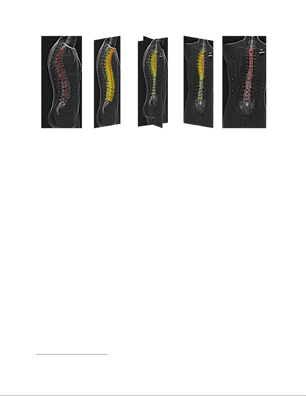
G E O M E T RY O F T H E E O S ® R A D I O G R A P H I C S C A N N E R A P R E P R I N T Benjamin N. Groisser Department of Mechanical Engineering T echnion-Israel Institute of T echnology Haifa, Israel bgroisser@campus.technion.ac.il Nov ember 4, 2021 A B S T R AC T The EOS ® scanner is a radiographic system that captures P A and lateral images in standing posture. The system is widely used in diagnosis and assessment of scoliosis, as it provides a lo w-dose alternativ e to traditional X-ray and can capture full-body images. Furthermore, spacial calibration between the tw o imaging vie ws is implemented in hardw are, facilitating 3D reconstruction of imaging targets. In this paper , a brief description of the system is follo wed by an explanation of the geometric relationship between 3D space and radiographic image space. 1 Introduction The EOS ® scanner is a unique radiographic system with se veral key features that hav e made it an k ey tool for diagnosis and assessment of scoliosis, in addition to use in assessment of e.g. knee arthritis. The physics of the multiwire chamber used to amplify the primary X-ray emissions are be yond the scope of this document; like wise, treatment of the clinical use of the system can be found else where[ 1 ]. Rather , what follo ws is a description of the rele v ant radiographic components and their relati ve positioning, which will then be used to deri v e simple formulae for projection and reconstruction between 3D space and image space. 2 Hardwar e 2.1 Slot Scanners Radiographic slot scanners are an alternative to standard digital radiography . While both technologies will produce a two dimensional image, there are significant dif ferences in construction that determine the properties of the output images. In the EOS ® scanner , X-ray emitters and detectors are mounted on an enclosed g antry . The emission beam profile is a highly collimated fan restricted to the axial plane; emitter and detector move in unison during the scan to traverse the field of vie w . Axial scan lines are then assembled to form a two dimensional image. This axial beam profile and matching detector has the effect of filtering out deflected radiation, helping to reduce imaging noise. 2.2 Geometry T wo X-ray emitters (with paired detectors) are mounted orthogonally . These elements are all linked to mov e in unison, such that frontal and lateral images are collected concurrently . The relative positions of the emitters and detectors are fixed and calibrated at installation. Note that each row of the image is perpendicular to the direction of tra vel of the gantry , and that each row on the frontal image corresponds to the same ro w in the lateral image. This implies that, for any gi ven point on one radiographic image, the epipolar line is exactly the corresponding ro w on the other image. A P R E P R I N T - N OV E M B E R 4 , 2 0 2 1 (a) Orthographic ov erhead view . (b) Perspectiv e vie w Figure 1: Renderings of EOS radiographic en vironment. Global coordinate axes are displayed at the origin: X (red) towards the frontal detector , Y (green) towards the lateral detector , and Z (blue) vertically upright. F or details on each symbol, consult Appendix A. Also note that, due to the fan pattern of the emission beam, the ef fectiv e image width at the isocenter is smaller than the physical detector width. The specific model used in this discussion generates square pix els; as such, images are true-scale on the plane of the isocenter . Structures located closer or f arther from the X-ray tube will e xperience magnification and parallax distortion. 3 Projections and Reconstructions As a matter of con vention, in the follo wing sections image ro ws will be numbered running from 0 as the top row to R as the bottom row . Like wise, columns run from 0 on the left edge to C on the right. A list of all the rele v ant parameters, along with representativ e values, can be found in Appendix A. Note that, although the physical detectors for frontal and lateral images are typically equal size, the dif ference in distance from the isocenter results in a lar ger ef fecti ve image width for the frontal image. 3.1 Projection Mapping points from 3D world space to radiographic image space can be achiev ed with a modified pinhole camera model. The pixel ro w in the frontal image v f is simply the vertical height of the point P z scaled by the pixel pitch λ z : v f = z 0 − P z λ z (1) where z 0 is the initial height of the emitter . T o find the projected location in homogeneous coordinates u 0 , transform the 3D point P in global coordinates into camera coordinates, then project into 2D with scaling factor ω .  u 0 f ω  =  f f 0 0 0 0 0 1 0     0 1 0 0 0 0 1 − P z 1 0 0 f f 0 0 0 1       P x P y P z 1    =  P y f f f f + P x  (2) 2 A P R E P R I N T - N OV E M B E R 4 , 2 0 2 1 Con verting from homogeneous coordinates to column index is performed by scaling by horizontal pitch, then offset to begin inde xing from the image edge: u f = C f 2 + P y f f λ f ( f f + P x ) (3) The same process can be used to find the pixel coordinates for the lateral image:    u l v l    =    C l 2 − P x f l λ l ( f l + P y ) ( z 0 − P z ) /λ z    (4) Note that the sign of the of fset (e.g. second term in Equation 3) will determine the orientation of the projected image. The con vention used here is radiographic standard: image is viewed from “behind” the imaging screen (e.g. in a posterior-anterior scan the patient left will appear on image right). 3.2 Reconstruction Radiographic reconstruction can be seen as the in verse of projection; points on lateral and frontal radiographs are reconstructed to find the corresponding point in 3D space. This is performed by back-projecting the points from the imaging screen to the X-ray source and finding the intersection between frontal and lateral projection lines. This can be formulated as solving a system of equations. First, con vert pix el coordinates into 3D location: x f = 0 , x l = λ l  C l 2 − u l  y f = λ f  u f − C f 2  , y l = 0 (5) Then solve the simultaneous equations P y = y f f f ( P x − f f ) P x = x f f l ( P y − f l ) ⇒  − y f f f f l − x l   P x P y  =  f f y f f l x l  (6) Solving for P x , P y can be easily performed e.g. with matrix inv ersion. Solving for P z is straightforward. If, due to rounding or labeling errors, the row index for the lateral and frontal images are not equal, a simple a verage can be used: P z = z 0 − λ z v l + v f 2 (7) 4 Examples 4.1 Synthetic Radiographs from CT In Figure 2, synthetic radiographs are generated from a clinical CT v olume. Data is provided by []. The same v olume is projected using two geometries: first, using a standard pinhole model to simulate standard Digital Radiography , and second, using the geometry described above. For each pix el in the image, the emission line from X-ray tube to detector is constructed. The segment that passes through the CT v olume is interpolated and integrated to compute the pix el value 1 . 1 It is possible to simulate different X-ray wa velengths by adjusting the integral. F or example, adding an aluminum filter might be modeled by applying a high-pass filter to the CT data, to selectiv ely amplify the contribution of dense material. 3 A P R E P R I N T - N OV E M B E R 4 , 2 0 2 1 (a) DR P A (b) EOS P A (c) DR LA T (d) EOS LA T Figure 2: Synthetic projections using clinical CT data. T op row sho ws Digital Radiography while bottom ro w demonstrates EOS geometry . In the case of DR the X-ray source (i.e. pinhole) is positioned in the center of the spine. Emitter distance to patient and detector are maintained between the two trials. 4.2 Reconstructing Corresponding Points An important use of stereo-radiographic systems is reconstructing 3D structures from planar images. One commonly used method is to find corresponding points in both images and then recover the 3D position using the process described in Section 3.2. T ypically , the dif ficult part of this process is to locate corresponding points in both images; this is often a challenging task requiring expert training. In spinal vertebrae, six points have been identified as readily identifiable in frontal and lateral projections[ 2 ]. In Figure 3 these points hav e been manually labelled for thoracic and lumbar vertebrae of a phantom spine model. These landmarks are then reconstructed, and a v ertebral mesh model is registered with six degrees of freedom (translation, rotation) to fit each set of landmarks. All v ertebral mesh models are rendered together in 3D, with radiographic images positioned at the isocenter . 5 Conclusions The EOS ® scanner is a hardware calibrated stereo radiographic system. The known geometry of the system facilitates projections from world coordinates to image coordinates, or reconstructions of corresponding landmarks from image space to world space. This is particularly useful for assessment of 3D anatomical structures in standing posture, such as the spine or lower e xtremities. 4 A P R E P R I N T - N OV E M B E R 4 , 2 0 2 1 (a) P A landmarks (b) LA T + model (c) P A,LA T + model (d) P A + model (e) P A landmarks Figure 3: Reconstructions of stereo-corresponding points. A spine model is also fitted for visualization. Note that these images are flipped relativ e to radiographic con v ention, for better alignment with 3D space. A Parameters As a representati ve e xample, the following parameters describe the EOS® system installed in the Pediatric Radiology department at the Hospital for Special Surgery (HSS) 2 . 1. d f : 1300mm - distance from frontal emitter to detector 2. f f : 987mm - distance from frontal emitter to isocenter 3. d l : 1300mm - distance from lateral emitter to detector 4. f l : 918mm - distance from lateral emitter to isocenter 5. w f : 450mm - width of frontal detector 6. w l : 450mm - width of lateral detector 7. λ x : 0.179363mm - horizontal pixel pitch for frontal image 8. λ y : 0.179363mm - horizontal pixel pitch for lateral image 9. λ z : 0.179363mm - vertical pixel pitch (shared by construction between frontal and lateral) 10. R : v aries - number of ro ws in each images (typically 7,000-10,000 for a full-body scan) 11. C f : 1895 - highest column index in frontal image (note there are C f + 1 total columns) 12. C l : 1763 - highest column index in lateral image (note there are C l + 1 total columns) References [1] T amas Illes and Szabolcs Somoskeo y . (2012) The EOS(TM) imaging system and its uses in daily orthopaedic practice. International Orthopaedics 36(7), 1325–1331. https://doi.org/10.1007/s00264-012-1512-y [2] Bernard Andre, Jean Dansereau, and Hubert Labelle. (1994) Optimized vertical stereo base radiographic setup for the clinical three-dimensional reconstruction of the human spine. Journal of Biomechanics 27(8). article. http://doi.org/10.1016/0021-9290(94)90219-4 2 Hospital for Special Surgery - 535 E 70th St, Ne w Y ork City , New Y ork 10021 5