Graph topology inference based on sparsifying transform learning

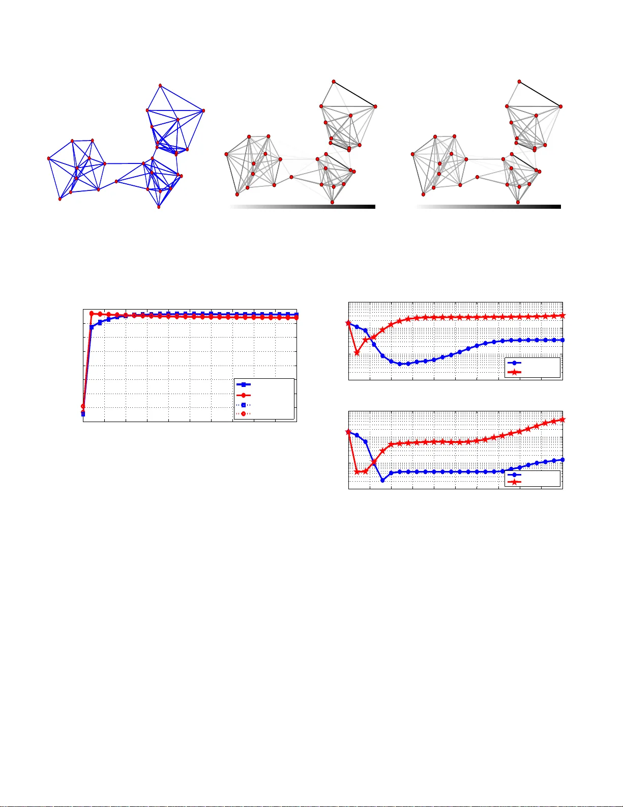
1 Graph topology infere nce based on sparsifying transform le arning Stefania Sardellitti, Member , IEEE , Sergio Barbarossa, F ellow , IEEE , a nd Paolo Di Lorenzo, Member , IEEE Abstract —Graph-based repre sentations play a k ey role in machine learning. The fundamental step in these represe ntations is the association of a graph structure to a dataset. In this paper , we propose a method that aims at finding a block sp arse repre sentation of th e graph signal leadin g to a modul ar graph whose Laplacian matrix admits the fo und dictionary as its eigen v ectors. The role of sparsity here is to induce a band- limited repre sentation or , equ iv alently , a modular structure of the graph. The proposed strategy is composed of two opti mization steps: i) learning an orthonorma l sparsifying transform fro m the data; ii) reco ver ing the Laplacian, and then topology , from the tra nsfor m. The first step is achiev ed through an i terativ e algorithm whose alternating intermediate solutions ar e expressed in closed form. Th e second step recov ers the Laplacian matrix from the sparsifyin g transform t h rough a conv ex opti mization method. Numerical re sults corroborate th e effectiveness of t h e proposed methods over both synthetic data and real brain data, used f or i nferring th e brain functi on ality network through experiments condu cted over patien ts affected by epilep sy . Index T erms —Graph learning, graph signal processing, sp ar - sifying t ransform. I . I N T R O D U C T I O N In ma ny machine learn ing application s, from b rain fu nc- tional a nalysis to gene regulator y networks or sensor network s, associating a graph-b ased representation to a dataset is a fundam ental step to extract relevant informatio n from the data, like detecting clusters or measuring node centrality . T he graph underly ing a given d ata-set can be r eal, as in the case of a sensor network, for example, or it can b e just an abstract descriptor of pairwise similarities. There is a large amount of work aimed a t learnin g the ne twork topolog y from a set of obser vations [1]. T ypically , th e graph topo logy reflects correlation s among signals defined over its vertices. Howe ver , looking o nly at corr elations may fail to capture the cau sality relations existing among the data. Alternative app roaches b uilt on par tial correlation [1], o r Gaussian graphica l mod els [2], [3 ] have been deeply in vestigated. The analy sis o f sign al defined over grap hs, or Graph Signal Processing (GSP) [4 ]–[7], has provided a fur ther strong impulse to the discovery of new technique s f or inf erring the graph topo lo gy from a set of observations. Som e GSP-b ased approaches make assumptions about the gra p h by enfo r cing pro perties such as spar sity and/or smoothne ss of the signals [8], [9], [ 10]. Specifically , Kalofo lias The authors are with the Departme nt of Information Engineeri ng, Elec- tronics, and T ele communica tions, Sapie nza Uni versi ty of Rome, V ia Eudos- siana 18, 00184, Rome, Italy . E-mails: { stefani a.sardell itti; serg io.barbarossa ; paolo.dil orenzo } @ uniroma1.it. This work has been supported by H2020 E UJ Project 5G-MiEdge, Nr . 723171. This paper was pre sented in part at the IEEE Global Conference on Signal and Information Processing, Global SIP , USA, Dec. 7-9, 2016. in [8] pro p osed a Lap lacian learnin g f ramework, for smo oth graph signals, by refor mulating the p roblem as a weight ℓ 1 - norm min imization with a log bar rier pen alty term on th e node degrees. Recen tly , the pro blem of learning a sparse, unweighte d , grap h Laplacian fr om smooth g raph signals has been modele d by Chepu ri et a l. as a rank ord ering p roblem, where the Laplacian is expressed in terms of a sparse ed ge selection vector b y assuming a prio ri knowledge of th e grap h sparsity le vel [9]. An alternative app roach con sists in definin g joint properties between signals and und erlying gr a ph such that the signal r e presentation is co nsistent with given statistical priors on laten t variables [10], [11]. Un d er the assumption that the obser ved field is a Gaussian Mar kov Ran dom Field (GMRF), who se pr ecision matrix is th e graph Lap lacian, Dong et al. [10] pro p osed a gr aph lea rning method th at fa vors sign al representation s that ar e smooth and co nsistent with the un d erlying statistical p rior model. Recen tly , in [11] Egilmez et al. propo sed a general fram ew ork where graph learning is formu lated as the estimation of different typ e s of graph La p lacian matrices by ad opting as minimization m etric the log-determin ant Bregman di vergence with an additional, sparsity promoting , ℓ 1 -regularization te r m. In [11] it is shown that such a prob lem corresp o nds to a maximu m a posterior i parameter estimation of GMRFs whose precision matrices are g raph Laplacians. I n case of d irected grap hs, Mei et al. prop osed algorithms for estimating the d irected, weighted adjacency matrices describin g the depen dencies among time series generated by systems of in teracting ag ents [ 12]. There are also som e r ecent works that focus on learning the graph topolog y fro m signals that diffuse over a graph [13], [14], [15]. Segarra et al. developed efficient spar se g r aph recovery algorithms for identifying the graph sh ift oper a to r (the adjacency m atrix or the normalized graph Laplacian) giv en only the eig e nvectors of the shift o perator [13]. These bases ar e estimated from the eigenv ectors o f the sample covariance matrix of stationa ry graph signals resulting from diffusion dynamics on the g raphs. Then the optimiza tion strategy m inimizes the shift- operator ℓ 1 -norm by imp osing complete o r partial knowledge of the eig en vectors of the empirical covariance matr ix . I n [14], Pasdeloup et a l. formu- lated the graph-in ference p roblem in a way similar to [1 3], albeit with a different matrix selection strategy , which aims at recovering a matrix modelin g a d iffusion process with out imposing the stru c ture of a valid Laplacia n to this matrix. Recently , Thanou et al. p roposed a gr aph learning strategy based on the assumption that the graph signals are g enerated from heat d iffusion pr ocesses starting fro m a few nodes of the graphs, b y e nforcing sparsity of the graph sign als in a 2 dictionary that is a concatenation of g r aph diffusion kernels at different scales [1 5]. The prob lem o f jointly estimating the dictio nary matr ix and the graph topolo gy f rom d ata has been recently tackled b y Y ankele vsky et a l. by taking into account the underly in g structure in bo th the signal and the manifold domains [16]. Specifically , two smoothness r egu- larization terms are introduc e d to descr ib e, respec ti vely , th e relations between the rows an d the co lumns of the data matrix . This leads to a dual grap h regu lar ized form ulation aime d at finding, jointly , the dictionary and the sparse data matrix. The graph Laplacian is then estimated by imposing smoothn ess of any signal represented over the estimated dictionary . Gi ven the observed graph sign al, the estimation of the Laplacia n eigenv ectors is concep tually equivalent to find ing a sparsifying transform [1 7]. A dictionary learn ing method for sparse coding incorpo rating a graph Lap lacian regulariza tio n term, wh ich enables the exploitation o f data-similarity , was developed in [18], while a diction ary learning method reinforcin g gr oup- graph structures was pr o posed in [19]. One of the ke y p roperties of the spectral r epresentation of signals defined over a graph is that the repr esentation depend s on the graph topolog y . The Graph Fourier T ransform (GFT), for example, is the p rojection of a signal onto th e space spanned by the eigen vectors of the graph Laplacian matrix. The main idea underlyin g our work is to associate a grap h to pology to the data in o rder to ma ke the observed signals ba n d-limited over the infer red graph o r , equiv alently , to make their spectral repr esentation sparse . Fin ding this spar se representatio n of a sign al o n a gra p h is in strumental to finding graph topo lo gies that are modular , i.e. graph s ch aracterized by densely interco nnected subsets (clusters) weakly intercon- nected with oth e r c lu sters. Modularity is in fact a structure that conv eys imp ortant informatio n. This is useful in all those applications, like c lu stering or classification, whose go al is to associate a label to all vertices belong ing to the same class or cluster . If we look at the labels as a signal de fin ed over the vertices o f a graph, we have a signal con stant with in each cluster and varying ar bitrarily acro ss different clusters. This is a typ ical band -limited signal over a graph. The p roposed approa c h is com posed of the following two main steps: i) lea r n the GFT b asis and the sp a rse sig n al rep r esentation join tly from the o bserved dataset; ii) infer the g r aph weighted Laplacian, and then the g raph to pology , from th e estimated L aplacian eigenv ectors. A nice feature of the pr oposed approach is that the first step is solved thr ough an alter nating o ptimization algorithm whose single steps are so lved in closed form . Furthermo re, the secon d step is cast as a conv ex prob lem, so that it can be efficiently solved. Wi th r espect to previous works, we make no assump tions about the stationarity o f the observed signal and we do not assume a ny d iffusion process taking place on the g raph. Interestingly , we find theo retical co nditions relating the sparsity of the grap h th at can be inferre d and the b andwidth (sparsity le vel) o f th e signal. T o a ssess the perfor mance of th e proposed approach es, we consider both synthetic and real data. In the first case, we know the groun d -truth graph and then we u se it as a benchm a rk. In such a case, we also comp are our m ethods with similar approaches, under different d ata models (e.g., band- limitedness, multivariate Gaussian r andom variables d escribed by an inverse Laplacia n covariance matrix, etc.). Then, we applied our method s to inf er the brain func tionality gr aph from electrocor ticograph y (ECoG) seizure data co llected in an epilepsy study [1], [20]. In such a case, the brain network is not directly observable and must be infer r ed by measur able ECoG signa ls. This r epresents an importa n t a pplication for the recently developed, g r aph-based learnin g meth o ds [21], [22]. By explo iting such meth ods, the hope is to g ain mor e insights about the u nknown me c h anisms un derlying some neur ological diseases such as, f or example, epilep tic seizur es. The rest of the pap er is organized as follows. Section II introdu c es the gr aph sign al mo dels and the topolog y learning strategy . Section III describes the first step of our method designed to learn jointly , a sub set o f the GFT basis an d th e sparse signal. T wo alter nativ e algorithms to learn th e Laplac ian matrix fr om the estimated ( incomplete) Fourier ba sis are then p resented in Sec tio n IV . Theor etical condition s on graph identifiability are discussed in Sectio n V . Numerical tests b a sed on bo th synthetic an d real data f rom an e pilepsy study , are then presented in Section VI. I I . L E A R N I N G T O P O L O G Y F RO M G R A P H S I G N A L S A. Graph signals model W e consider an undir e cted graph G = {V , E } consisting of a set of N vertice s (or nodes) V = { 1 , . . . , N } alon g with a set of edges E = { a ij } i,j ∈V , such that a ij > 0 , if there is a link between node j and node i , or a ij = 0 , o therwise. W e denote with |V | the cardinality of V , i.e. the nu mber of elemen ts of V . Let A den ote the N × N ad jacency , symmetric matrix with entrie s the edge weights a ij for i , j = 1 , . . . , N . The (unno rmalized) graph Laplacian is d efined as L := D − A , where the degree matrix D is a diagonal matrix whose i th diagona l e n try is d i = P j a ij . Since G is an undirected gr aph, the associated Lap la c ian matrix is symmetric and positiv e semidefinite and ad mits th e e ig endecom position L = UΛU T , where U collects all the eigenvectors { u i } N i =1 of L , whereas Λ is a diagona l matrix containin g the eigenv alues o f L . A signal y on a grap h G is defined as a mapping from the vertex set to a comp lex vector o f size N = |V | , i. e. y : V → C . For un directed g raphs, th e GFT ˆ y of a graph signal y is defined as the pro jection o f y o nto the subspa ce spanne d by the eigen vectors o f the Laplacian m atrix, see e.g . [ 4], [ 6], [7]: ˆ y = U T y . (1) A band -limited grap h sign al is a signal whose GFT is sparse. Let us d enote these sig n als as y = U s (2) where s is a sparse vector . One o f the main motivations for projecting the sign al y onto th e subspace spa nned by th e eigenv ectors of L , is tha t these eig en vectors encod e so me of the graph topological features [23], [24]. In par ticular , the eige n vectors associated to the smallest eigen v alues o f L identify graph clusters [23]. Hence, a band-limited sign al with support o n th e lowest in dices is a signal that is smooth within 3 clusters, while it can vary ar bitrarily across clusters. More formally , gi ven a sub set of in dices K ⊆ V , we introdu c e the band -limiting op e rator B K = UΣ K U T , wher e Σ K is a diagona l m atrix defined as Σ K = Diag { 1 K } and 1 K is the set indicator vector, wh o se i -th entry is e qual to one if i ∈ K , and zero otherwise. Let us assume th at s ∈ R N is a |K| -spar se vector, i.e. k s k 0 ≤ K , where th e l 0 -norm counts th e n umber o f n on- zeros in s and K = |K | . W e say that y is a K - band-limited graph signal if B K y = y , or, equiv alently , if y = U s , where s is a |K | - sparse vector [ 25]. Th e observed signal y ∈ R N can be seen as a linear comb ination o f colum ns f rom a d ic tio nary U ∈ R N × N . Collecting M vectors s i ∈ R N in the ma trix S ∈ R N × M , we assume th at the signals s i share a co m mon support. Th is implies that S is a b lock-sparse matrix having entire r ows as zeros o r nonzer os. W e d efine the set o f K -b lock sparse signals [26], [ 27] as B K = { S = [ s 1 , . . . , s M ] ∈ R N × M | S ( i, :) = 0 , ∀ i 6∈ K ⊆ V , K = |K|} (3) where S ( i, :) deno tes the i th row of S . Hen ce, by introducin g the matr ix Y ∈ R N × M with columns th e M obser ved vectors y i , we g et the c o mpact form Y = US whe r e S ∈ B K . B. Pr oblem formulation In this p aper we propo se a novel strategy to learn , jointly , the ortho normal tra nsform ma tr ix U , the sparse grap h sign al S and th e un derlying g raph top o logy L . Altho u gh the matrices U , S and L are n ot uniq uely id entified, we will devise an efficient algorithm to find optim a l solutions that minimize the estimation error . Before f ormulating ou r pr oblem, we introdu c e the space of valid combin atorial Laplacian s, i.e. L = { L ∈ S N + | L 1 = 0 , L ij = L j i ≤ 0 , ∀ i 6 = j } (4) where S N + is the set of real, symmetric and positive semidef- inite m atrices. In princ ip le, our g oal would be to find the solution of the f ollowing optimizatio n proble m min L , U , Λ ∈ R N × N S ∈ R N × M k Y − US k 2 F + f ( L , Y , S ) ( P ) s.t. a ) U T U = I , u 1 = b 1 b ) LU = UΛ , L ∈ L , tr ( L ) = p c ) Λ  0 , Λ ij = Λ j i = 0 , ∀ i 6 = j d ) S ∈ B K , where: the objectiv e function is the sum of the data fitting error plus th e function f ( L , Y , S ) enabling, as we will see in Section IV , the r e c overing of a gr a p h top ology which reflects the smoothn ess o f the o bserved graph sign als; the constra int a) forces U to be un itary and includ es a vector pro p ortional to the vector of all ones; b ) con strains L to p ossess the d e sired struc- ture and imposes that U and Λ are its eig en-deco m position; the trace con straint, with p > 0 , is u sed to av oid the trivial solution; c) forces L to be positive semid efinite (an d Λ to be diago nal); finally , d) enfo rces the K -blo ck sparsity of the signals. Howe ver , p r oblem P is non-co n vex in both the objective fun c tion and the constrain t set. T o make the p roblem tractable, we devise a strategy that deco uples P in two simp ler optimization prob lem s. The pro posed strategy is rooted on two basic steps: i) first, giv en the observation matrix Y , learn the orthon ormal tr a n sform matrix U and the sparse sign al matrix S jointly , in order to min imize the fitting er r or k Y − US k 2 F , subject to a block -sparsity constraint; ii) second, given U , infer the graph Laplacian matrix L th at admits the column of U as its eigenvectors. While the theoretical proo f of co n vergence of this double-step approa c h is still an open question , th e effecti veness o f the propo sed strategy h as been corro b orated by extensi ve nu merical results over both simulated and real data. In the n ext sectio n s, we will develop alterna tive, suboptimal algorithm s to solve the p r oposed graph inference pro blem a n d we will present the n umerical r esults. I I I . L E A R N I N G F O U R I E R BA S I S A N D G R A P H S I G N A L S J O I N T L Y In this section we describe the first step of the propo sed graph recovering strategy , aimed at learning the p air o f ma- trices ( U , S ) join tly , u p to a multiplicativ e rotation matrix . Observe that, since U ∈ R N × N is full rank, if U is known, recovering S fr o m Y is easy . Ho wev er , in o ur case, U is unknown. He n ce, r ecovering b oth S and U is a cha llenging task, which is prone to an ide n tifiability prob lem . T o solve this task, we use a method conceptually similar to sparsifying transform learn ing, assum ing a unitary transfo rm [28], with the only difference that we enfo rce block -sparsity and we impose, a pr io ri, that one of the eigenvectors be a c o nstant vector . Mo re specifically , we set u 1 = b 1 , with b = 1 / √ N . Because of the u nitary pro perty of U , we can write k Y − US k 2 F = k U T Y − S k 2 F . Our g o al is to find the blo c k-sparse columns { s i } M i =1 , and the Fourier basis orthonorm al vector s { u i } N i =1 , minimizing the sparsification error . Ther efore, gi ven the train in g matrix Y ∈ R N × M , motivated by the origin al problem P , we formulate the following o ptimization prob lem: min U ∈ R N × N , S ∈ R N × M k U T Y − S k 2 F ( P U,S ) s.t. U T U = I , u 1 = b 1 S ∈ B K . (5) Although the objective fu nction is con vex, p roblem P U,S is non-co n vex due to the nonco n vexity of both the orthon ormality and sparsity co n straints. In th e following, inspir e d by [ 28], we propo se an algor ithm to solve P U,S that alternates between solving for the blo c k-sparse signal matr ix S and for the orthon ormal transform U . A. Alternatin g op timization algo rithm The prop osed appro ach to solve the above n on-conve x problem P U,S alternates between the min imization of the 4 Algorithm 1 : Learn ing Fourier basis and graph signals Set U 0 ∈ R N × N , U 0 T U 0 = I , u 1 = b 1 , k = 1 Repeat Find ˆ S k as solution of S k in (7); Compute the optimal point ˆ U k as in (9); k = k + 1 ; until con v erg ence objective f unction with respect to S and U at each step k , iterativ ely , as follows: 1. ˆ S k , arg min S ∈ R N × M k ( ˆ U k − 1 ) T Y − S k 2 F ( S k ) s.t. S ∈ B K 2. ˆ U k , arg min U ∈ R N × N k U T Y − ˆ S k k 2 F ( U k ) s.t. U T U = I , u 1 = b 1 . The algorithm iterates until a termination criter io n is met, within a prescribed accuracy , as summar ized in Algo rithm 1. The in te r esting feature is that the two n on-convex problems S k and U k admit closed-f orm solu tions. Theref o re, bo th steps of the ab ove algor ithm can be p erforme d exactly , with a low computatio nal cost, as follows. 1) Computa tion of the critical p oint ˆ S k : T o solve proble m S k we need to d efine the ( p, q ) -mixed no rm of th e m a trix S as k S k ( p,q ) = N X i =1 k S ( i, :) k q p ! 1 /q . (6) When q = 0 , k S k ( p, 0) simply co unts the number of nonzero rows in S , whereas for p = q = 2 we g e t k S k 2 (2 , 2) = k S k 2 F . Hence, we reform ulate problem S k as in [26], to obtain the best block-spa rse approxim ation of the matrix S as follows arg min S ∈ R N × M k ( ˆ U k − 1 ) T Y − S k 2 F ( S k ) s.t. k S k (2 , 0) ≤ K (7) where we fo rce the rows o f S to be K -blo ck sparse. The solution of this problem is simply obtained by sorting the rows of ( ˆ U k − 1 ) T Y by their l 2 -norm and then selecting the rows with largest no rms [26]. 2) Compu tation of the critical point ˆ U k : T h e optimal transform u pdate f o r the transfo rm matrix U k is pr ovided in the following propo sition. Pr o position 1: Defin e ¯ Y k = Y ( S k ) T , Z k = [ ¯ y k 2 , . . . , ¯ y k N ] , where ¯ y k i represents the i th co lumn o f ¯ Y k , and Z k ⊥ = PZ k with P = I − 11 T / N . If r = r ank ( Z k ⊥ ) , we hav e Z k ⊥ = XΣV T = [ X r X s ] ΣV T (8) where the N × r m atrix X r contains as colu mns the r left- eigenv ectors associated to th e non-zer o singular values of Z k ⊥ , X s is an orthono rmal N × N − r matrix selected as belong ing to the nullspa c e of th e matrix B = [ 1 T ; X T r ] , i. e . BX s = 0 . The optimal solution of the n o n-conve x problem U k is then ˆ U k = [ 1 b ¯ U ⋆ ] (9) where ¯ U ⋆ = X − V T and X − is obtained b y r emoving from X its last column. Proof. See Appendix A. Of cou rse, th e pair of m atrices ( U , S ) so lv ing (5) can only be fo und up to th e multiplicatio n by a unitary matrix W that preserves the sparsity of S . In fact, US = UW W T S := ˆ U ˆ S , where W is a unitary matrix , i.e., W W T = I . I n the next section, we will take into acc o unt the presence of this unknown r o tation matrix in the recovery of the g r aph topolog y . Nev ertheless, if the grap h signals assume values in a discrete alphabet, it is p ossible to de-rotate the estimated tran sform ˆ U by using the ad a p ti ve, iterative alg orithm d ev eloped in [ 29], based on the sto c h astic gra d ient approx im ation, as sh own in Section VI. I V . L E A R N I N G T H E G R A P H T O P O L O G Y In this section we pr o pose a strategy a im ed at identify ing the topolo g y of the graph by learnin g the Lap lacian matr ix L from the estimated transform matrix ˆ U . Of course, if w e would know th e eig en value and eigenvector m atrices of L , we could find L by solv ing LU = UΛ . (10) Howe ver , from the algor ithm solving pro b lem (5) we can on ly expect to find two matrices ˆ U = UW and ˆ S = W T S , where W is a unitary matrix that preserves the block-sp a r sity of S . This means that, if we take the pro d uct L ˆ U , we get L ˆ U = LU W = UW W T ΛW . (11) Introd u cing the matrix C = W T ΛW  0 , we can write L ˆ U = ˆ UC . (12) Furthermo re, h a ving supposed th at th e o b served graph sign als are K -band lim ited, with |K| = K , we can only assume, from the first step of the algorithm , knowledge o f th e K co lumns of ˆ U associa te d to the observed signal subspace. Under this setting, the constraint in (12) re d uces to L ˆ U K = ˆ U K C K (13) with C K ∈ R K × K , C K = Φ − 1 Λ K Φ  0 , Φ a un itary m a tr ix and Λ K the diago nal matrix obtained by selecting th e set K of diagonal entries o f Λ . For the sake of simplify ing the optim ization prob lem P , th e graph learning problem can b e formulated as fo llows min L ∈ R N × N , C K ∈ R K × K f ( L , Y , ˆ S ) ( P f ) s.t. L ∈ L , tr ( L ) = p L ˆ U K = ˆ U K C K , C K  0 ) , X ( ˆ U K ) with L defined as in (4) . Different cho ices for the o bjectiv e function f ( L , Y , ˆ S ) h av e been proposed in the literature, such as, fo r example: i) f ( L ) = || L || 0 , as in [13], or ii) f ( L , Y ) = tr ( Y LY T ) + µ || L || F , as in [1 0]. In the first case, the goal was to recover the spar sest gr aph, given the eigen- vectors o f the shift ma tr ix, estimated via principal comp o nent analysis (PCA) of the samp le covariance o f grap h signals diffused on the network . I n th e second case, the goal was to 5 minimize a lin ear comb ination of th e l 2 -norm total variation of the ob served sign al Y , measuring the signal smo othness, plus a Frobenius norm term, specifically added to control (throu g h the co e ffi cient µ ≥ 0 ) the distribution of the off- diagona l entries of L . Note that, because o f the con straint on the L a p lacian trace, setting µ to large values penalizes large degrees and leads, in the limit, to dense g raphs with constan t degrees acro ss th e n odes. In this paper, our goal is to infe r a grap h topology tha t gi ves rise to a ban d-limited sign al, co nsistent with the observed signal. This infer e n ce is based on the joint estimation of the |K| -sparse signal vecto r s i and the Lap lacian e igen vectors jointly . T o this end, we pr opose two alternative choices f or the objective function, leading to the f ollowing two algorithms. A. T otal va riation ba sed g raph learning The T otal V ariation Graph Learn in g (TV - GL) algo rithm, is formu late d as follows min L ∈ R N × N C K ∈ R K × K f 1 ( L , Y , µ ) , T V ( L , Y ) + µ k L k 2 F ( P f 1 ) s.t. ( L , C K ) ∈ X ( ˆ U K ) where TV ( L , Y ) = P M m =1 P N i,j =1 L ij | Y im − Y j m | repre- sents th e ℓ 1 -norm total variation of the observed signal Y on the graph. Minimizing this ℓ 1 -norm tends to disco nnect nod es having distinct sign al values and to co n nect n odes h a ve similar values, wher eas the Frobenius norm co ntrols the sparsity of the off-diago nal entries of L ; the con straint o n the Lap lacian trace in X ( ˆ U K ) is instrumenta l to av oid the tri vial solution by fixing the l 1 -norm of L . Note that this constrain t can be read as a sparsity co nstraint on L , since tr ( L ) = k L k 1 , and th e l 1 norm rep resents the tightest relaxatio n of the l 0 norm. The coefficient µ is used to con trol the g raph sp a rsity: if µ increases the Fro benius n orm of L ten ds to d ecrease and, because of the trace constraint, this leads to a mo re uniform distribution of the o ff-diagonal entries so that the numb er of edges increases; on the contrary , as µ goes to 0 , the grap h tends to be m ore and more sparse. Problem P f 1 is con vex since both feasib le set and objectiv e function are con vex. B. Estimated- signal-aid ed g raph learnin g W e pr opose n ow an alternative method, which we name Estimated-Signa l- Aided Grap h Lea r ning (ESA-GL) alg orithm. In this case the signals ˆ S estimated in Algorithm 1 are used in the gr aph recovering method . T o motiv ate this meth od, we begin ob serving th at tr ( Y T LY ) = tr ( S T K Λ K S K ) = tr ( ˆ S T K C K ˆ S K ) (14) where S K contains the rows with index in the sup p ort set of the graph signals, whereas ˆ S K = Φ T S K are the graph signals estimated by Alg orithm 1. Therefo re, an altern ativ e form u la- tion of problem P f aiming at minimizing the smoo thing ter m in (14), is min L ∈ R N × N C K ∈ R K × K f 2 ( L , ˆ S K , µ ) , tr ( ˆ S T K C K ˆ S K ) + µ || L || F ( P f 2 ) s.t. ( L , C K ) ∈ X ( ˆ U K ) . Also in this case th e form ulated problem is convex, so that it can be efficiently solved. V . L A P L AC I A N I D E N T I FI A B I L I T Y C O N D I T I O N S Before assessing the g o odness o f th e proposed in ference algorithm s, in th is section we in vestigate the co nditions u nder which the Laplacian matrix can be recovered uniquely . Inter- estingly , the deriv ations lead to an interesting relatio n between the ban dwidth of the sign al and the sparsity of the gr a ph. W e start looking for the condition s under which the feasible set X ( ˆ U K ) of prob lems P f 1 and P f 2 reduces to a singleton. T o derive closed for m b ounds for the identifiability cond itions of the Laplacian matrix, we need to assume th a t the transform matrix is perf e c tly known, so that ˆ U K = U K . Even thou gh these are ideal co nditions b ecause our pr o posed algorithms are on ly able to recover U K up to a rotatio n , the closed forms provide a m eaningfu l insight into the relatio n between grap h sparsity an d signal bandwidth . Furthermore, we remark that it is possible to r ecover the matrix U K with no rotation in the case wher e the signal values belong to a known d iscrete set, by usin g the blind algorithm of [29], as shown in Section VI. Assume w .l. o.g. that the K eig en vectors of U K are sorted in increasing o r der o f their corre sp onding eigenv alues so th at 0 = λ K , 1 ≤ λ K , 2 ≤ . . . ≤ λ K ,K with Λ K = diag ( λ K ) . As a consequ ence, th e conv ex set X ( U K ) of problem s P f 1 and P f 2 , can be written as X ( U K ) ,                          a) LU K = U K Λ K b) L1 = 0 c) L ij = L j i ≤ 0 , ∀ i 6 = j d) λ K , 1 = 0 , λ K , 2 ≥ 0 e) λ K ,i +1 ≥ λ K ,i , i = 2 , . . . , K − 1 f) tr ( L ) = p (15) where con ditions b) − e) imp ose the d esired Laplacian struc tu re to L and f ) fixes its l 1 -norm b y av oiding the trivial solution. For the sake of simp licity , we focus on th e c ase where the subset K consists o f the ind ices associated to the first K columns of U ; otherwise one can follow similar argumen ts for any subsets of indices by p roperly rewriting conditio n s d) − e). As shown in Appen dix B, we can redu ce equation s a)-c) and f ) in ( 15) to th e following comp act form : Fx = b , x ∈ R N ( N − 1) / 2+ K − 1 + (16) where we defined x , [ − z ; ¯ λ ] ; z , vech ( L ) ∈ R N ( N − 1) / 2 − ; vech ( L ) the half-vecto r ization of L obtain ed by vectorizin g only the lower tr ia n gular part (except the diag o nal entries) of L ; R + and R − the sets of, respectively , nonn egati ve and nonpo siti ve real n u mbers; ¯ λ , { λ K ,i } ∀ i ∈K − where, assuming 6 the entries of λ K in increasing order, the in d ex set K − is obtained b y removing from K the first in dex correspo n ding to λ K , 1 ; b = [ 0 K N ; p ] ; an d , finally , the coefficient matrix F ∈ R m × n , with m = K N + 1 , n = N ( N − 1) / 2 + K − 1 is defined in Appendix B, eq uation ( 40). Note that the rank q o f the coefficient matrix F ∈ R m × n is q ≥ K − 1 and q ≤ min { n, m } . Pr o position 2: Assume the set X ( U K ) to be fea sible, then it holds: a) K − 1 ≤ rank ( F ) ≤ K N + 1 for K ≤ N 2 − 2 N − 1 and K − 1 ≤ rank ( F ) ≤ N ( N − 1) / 2 + K − 1 for K > N 2 − 2 N − 1 ; b) if rank ( F ) = K N + 1 a nd K = N 2 − 2 N − 1 , or rank ( F ) = N ( N − 1) / 2 + K − 1 a nd K > N 2 − 2 N − 1 , the set X ( U K ) is a singleton. Proof. See Section A in Appendix C. By using some prop erties about nonnegative solutions of un- derdeterm ined system s [ 3 0], un der the assumption of existence and uniquen ess o f solutio n s for the system (16), we can d eriv e the fo llowing condition relating graph sparsity and sign al bandwidth K . Pr o position 3 : If the set X ( U K ) with K < N 2 − 2 N − 1 , is feasible a nd { x | Fx = Fx 0 , x ≥ 0 } is a singleton for any nonnegative s -sp arse signa l x 0 , then N 2 − 2 N − 1 > K ≥ 2 s/ N and k A k 0 ≤ K ( N − 2) + 2 c wher e c is th e numbe r o f connected compon ents in the graph. Proof. See Section B in Appendix C. Note that if we assume th e graph to b e disconne c te d , i.e. c > 1 , the up per boun d on the graph sparsity tend s to incr ease to compen sate for the co nnectivity loss. V I . N U M E R I C A L R E S U LT S In this sectio n, we present some n u merical results validating the effecti veness of the propo sed graph-learnin g strategies for both synthetic and real-world g r aphs. In all numerical experiments we solved the proposed optimization p roblems by using the con vex optimization pack age CVX [ 3 1]. P erf ormance over synthetic data Let us con sid e r the graph in Fig. 1 a comp osed of N = 30 nodes forming 3 clu sters of 10 nod es each. T o start testing the ef fectiveness of the prop osed graph inferenc e stra tegies, in Fig. 1 we illustrate an example of graph topolog y recovery resulting by using the T V -GL a nd ESA-GL algo rithms. The color on ea c h edge enco des the strength of th at edge. W e can observe tha t, learnin g the Fourier ba sis using Algorith m 1 , both algorithm s are able to ensure a g ood topology re c overy . As a statistical test, we run simulatio n over 100 indepe n dent signal m atrix realization s, with N = 30 a nd M = 15 , assuming K = 3 for the b lock spa r sity an d setting tr ( L ) = N . As a first perfo rmance measur e, we measur e d th e corre la tio n coefficient b etween the true L a placian entries L ij and their es- timates ˆ L ij : ρ ( L , ˆ L ) , P ij ( L ij − L m )( ˆ L ij − ˆ L m ) √ P ij ( L ij − L m ) 2 q P ij ( ˆ L ij − ˆ L m ) 2 where L m and ˆ L m are the average values of the entr ies, r espectiv ely , of the true and estimated Laplacian matrices. Note that, because of the Laplacian matrix structure, we always h av e L m = ˆ L m = 0 . In Fig. 2, we plot the average correlation coefficient ¯ ρ ( L , ˆ L ) vs. the pen alty co efficient µ , where ˆ L is computed by apply in g the total variation based (TV -GL) or the estimated-signal aiding graph-lea rning (ESA-GL) algorithms. T o get in sight into the prop osed algorith ms, we consid e r ed both cases when the Fourier transform matrix U is a priori known or w h en it is estimated b y usin g Algorithm 1 . From Fig. 2, we notice that both metho ds are able to ensur e high av erage co rrelation co e ffi cients. Fur th ermore, we can observe a h igh ro bustness of th e TV - GL metho d to th e ch oice of the penalty parameter with respect to the ESA-GL algor ithm. By comparin g the cur ves o btained by assuming perf ect knowledge of U with those d eriv ed b y estimating it thr ough Alg orithm 1 , we can also n o tice that the pe rforman ce loss d ue to estimation errors is negligible. In ge neral, the c h oice of µ has an impa c t on the final r esult. T o assess th is impact, in Fig. 3 we illustrate the av erage normalized recovery error ¯ E 0 versus the penalty coefficient µ . The error ¯ E 0 represents the fraction of misidentified edges and is defin ed as k A − ˆ A b k 0 N · ( N − 1) where A an d ˆ A b are, respectiv ely , the grou n dtruth and the rec overed binary adjacency matrices. The b in ary matrix ˆ A b has been obtaine d by thresho ld ing the entries of the r ecovered matrix ˆ A with a threshold equal to half th e average values of the elements of ˆ A . W e consid er both cases where the Fourier b asis vectors are estimated (upp er plot) or a-prior i perfectly known (lower plot). Under this last setting, we solve prob lem P f 1 and P f 2 by assuming ( L , C K ) ∈ X ( U K ) . Th ereby , we solve p roblem S k , b y supposing pe r fect knowledge of U , in or d er to calcu late the estimated signals ˆ S , needed as input to solve problem P f 2 . W e can see that the percentage o f incor rect edg e recovery can be in the or d er of 0 . 4% . Furtherm o re, co m paring the TV -GL algorithm with the ESA-GL, we can observe that TV - G L tends to perform better . P erf ormance versus signa l ba ndwidth T o ev aluate the im pact o f the signal bandwidth K o n the g r aph recovery strategy , we illustrate some numerica l results perfor m ed on random graphs composed of N = 30 nodes with 3 clusters, each o f 10 nodes, by av eraging the final results over 100 gr a phs and signal matrix realizations for M = 15 . W e consider b oth cases of exactly o r only approx imately (or comp ressible) ba ndlimited graph signals [32]. W e recall that a vector is co mpressible if the error of its b est k -ter m appr oximation decay s qu ickly in k [ 32]. W e generate each b and-limited signal s i for i = 1 , . . . , M as s i ( k ) ∼ N (1 , 0 . 5 ) for all k ≤ K , and s i ( k ) = 0 for all k > K . In Fig. 4a we plot the a verage recovery error ¯ E 0 (upper plot) and the average recovery error ¯ E F (lower plot), defined as k A − ˆ A k F N · ( N − 1) , vs. the signal bandwid th K . W e selected for each K the optimal co e fficient µ minimizing the average recovery err o r . W e can observe th a t the error tends to increase as the sign a l bandwid th K g ets larger than the n umber of c lu sters, equal to K = 3 . Finally , in Fig. 4b we repo rt the av eraged recovery er r ors in case of compressible g raph signals, generated as s i ( k ) ∼ N (1 , 0 . 5 ) for all k ≤ K v and s i ( k ) = ( K v /k ) 2 β for all k > K v , with β = 2 , K v = 5 [33]. W e can observe th at for the TV -GL method the average recovery err ors increases as the signal bandwidth in creases, wh ile the min imum is achieved for 7 OR IGI NAL (a) TV−GL 0.017 0.32 (b) ESA-G L 0.018 0.36 (c) Fig. 1: Ex amples of grap hs learning: ( a ) orig inal graph; ( b ) rec overed grap h through TV -GL algo rithm with µ = 2 ; ( c ) recovered graph throug h ESA-GL algorith m µ = 0 . 1 . 0 0.5 1 1.5 2 2.5 3 3.5 4 4.5 5 0.2 0.3 0.4 0.5 0.6 0.7 0.8 0.9 1 µ ¯ ρ ( L , ˆ L ) M = 15, K = 3 ˆ U , TV-G L ˆ U , ESA-G L U , T V-G L U , E SA-G L Fig. 2: A verage corr elation co efficient versus th e param eter µ . K = 5 , since K v = 5 represen ts the app roximated g raph signal bandwidth. Ad ditionally , th e ESA- GL m ethod seem s to reach minim um values quite similar to those o f the TV -GL algorithm for K close to 5 . P erf ormance over real data In this section we test our method s over real d ata for recovering the brain fu nctional con nectivity network associated to ep ilepsy . Understan d ing how this abno rmal neuron al activity emerges and fro m what epileptog enic zone, would help to refine surgical techniques an d devise novel therapies. The diagn osis inv olves compar ing ECoG tim e series obtain e d f rom the patien t’ s brain be fore and after on set of a seizure. Epilepsy data description W e used the datasets taken from experiments conduc ted in an epilepsy study [20] to infer th e brain func tio nal activity map. The data were collected fr o m a 39-yea r-old fema le subject with a case o f intrac tab le epilep sy at the University of California, San Francisco (UCSF) Epilep sy Cen te r [ 20]. An 8 × 8 electro de grid was implanted in the co rtical surface 0 0.5 1 1.5 2 2.5 3 3.5 4 4.5 5 10 −3 10 −2 10 −1 10 0 µ ¯ E 0 ˆ U , T V-GL ˆ U , ES A-GL 0 0.5 1 1.5 2 2.5 3 3.5 4 4.5 5 10 −3 10 −2 10 −1 10 0 µ ¯ E 0 U , TV-G L U , ES A-GL Fig. 3: A verage recovery error vs. the co efficient µ , using estimated Fourier b asis vectors (up per p lot) and a - priori knowledge of the Fourier tran sform ( lower plot). of the subject’ s brain and two a ccompanying strips of six electrodes each wer e imp lanted d eeper into the br ain. This combined electro des network recorde d 7 6 ECoG time series, consisting o f voltage levels in the vicinity of each electro de, which are ind icati ve of the levels of local brain activity . Physicians recorded data fo r 5 consecutive days and ECoG epochs containing eight seizure s were extracted fr om the record. The time series at each electro de w e re first passed throug h a band pass filter with cut-off frequ encies of 1 and 50 Hz and two tempo r al inte r vals of inter est were picked f or analysis, na m ely , the preictal a n d ictal intervals. The preictal interval is defined as a 10 -seco nd interval preced in g seizure onset, while th e ictal inter val cor responds to the 10 -secon d immediately af te r the start of a seizure. For f urther details on data acquisition see [20]. 8 2 4 6 8 10 12 14 16 0.05 0.1 0.15 0.2 0.25 K ¯ E 0 Ban d limited sign a ls ˆ U , TV-G L ˆ U , ES A-GL 2 4 6 8 10 12 14 16 0 0.005 0.01 0.015 K ¯ E F ˆ U , TV-G L ˆ U , ES A-GL (a) 2 4 6 8 10 12 14 16 0.08 0.1 0.12 0.14 0.16 0.18 K ¯ E 0 Co mp ress ible sign a ls ˆ U , T V-GL ˆ U , ES A-GL 2 4 6 8 10 12 14 16 0 0.005 0.01 0.015 K ¯ E F ˆ U , T V-GL ˆ U , ES A-GL (b) Fig. 4: A verag e recovery errors versus K for a) ban dlimited g raph signals; b) f o r compressible g raph sign als. Recovery o f brain function al activity graph Since the o b served signal is h ighly n on-stationar y , following the same appro ach d escribed in [20], b efore ru n ning our algo- rithms we divide the 10 second s inter val into 20 overlapping segments of 1 second, so th at each segment overlaps with th e previous one by 0 . 5 second s. The reaso n is that within a one second interval, the b rain activity is appro ximately stationary . After this segmen tation, our goal is to infe r the network topolog y for each segmen t. W e de n ote by Y ∈ R N × M the observed da ta matrix, with N = 7 6 and M = 400 . Before ap plying ou r infer ence algorith m, we filter the data to reduce the effect of noise, using the metho d propo sed in [34] where an optimal shrink age of the empirica l sin g ular values of the observed matr ix is app lied. Gi ven the com pressed signal matrix ˆ Y , we pr oceed by ru nning first Algorithm 1 to estimate the transform matrix ˆ U and, thereafte r, we recover the brain network to pology by using th e T V -GL alg orithm. In Fig. 5 we show two examples of graph s learn ed from the observed (and filtered) data. They refer, respectively , to the pre-ictal inter val 19 and ictal interval 1 . W e can no tice how the num b er of edges changes dramatica lly , showing that the network c o nnectivity tends to decrease at seizure onset. This behavior is espec ially evident in the bottom corner of the g rid closest to the two strips of electrodes which were located close to where the seizure was suspec te d to ema n ate so that in this region the connectivity of the network tends to decre ase at seizure onset, as observed in [20]. The p r oblem in associating a grap h topolog y to a set of signals is that we d o n ot k now the grou nd truth. T o validate our appro a c h fro m a purely data- o riented perspective, we used the following appro ach. W e con sider the observations taken in two intervals, say pre-ictal inter val 19 and ictal interval 1 . The g r aphs inferre d in these two cases are the one s depicted in Fig. 5. Then , we assume that we observe on ly the signals taken f rom a sub set of electrodes and we ask ourselves whether we can recover the signals over the unobserved electro des. If the signals is band- limited over the recovered g raph, we can apply sampling theo ry fo r graph signals, as e.g. [25], to r ecover the u nobserved signals. Then we comp are what we are able to reconstru ct with wh a t is indeed known. W e use a greedy sampling strategy using an E-optimal d esign criterion [3 5], selecting the bandwidth provided by our transfor m learn ing method, which is equ al to 6 0 for th e pre-ictal interval, and to 64 f o r the ictal inter val. Th e num ber of electro d es assumed to be observed is chosen e qual to the ba n dwidth in both cases. For each tim e instant, we use a ba tch co nsistent recovery method that recon structs th e signals from the collected samp les [see eq. (1 .9) in [35]]. In Fig. 6, we illustrate the true ECoG signal present at no de 72 (black line) an d what we are able to reconstruc t (g reen line) f rom a subset of node s that do es not contain no de 72 . W e repeated this oper ation for bo th the pre- ictal (top ) and th e ictal (b ottom) phases. As we can no tice fro m Fig. 6, the reco nstructed signa l is very close to the real signal, in bo th phases. This m e ans that, e vidently , the inferred gr aphs are close to reality , because otherwise the samplin g th eory would have been based on a wrong topolog y assumption and then it could not lead to suc h a goo d pr e d iction. Comparison with GSP -based to pology inference methods. In this section we compare th e p erforman ce of our algorithms with recen t GSP-based algorithms, n a m ely the methods used in [1 3], [8], [10] to identify the Laplacian m atrix exploiting the smoothne ss of g raph signals. T o make a fair comparison , we considered fo r all method s the com binatorial Laplacian ma tr ix. T o implem ent the algor ithm SpecT emp prop osed in [13], we need to solve the following p roblem min L , L ¯ K , L ′ , λ k L k 1 ( P s ) s.t. L ∈ L L ′ = L ¯ K + P K k =1 λ k ˆ v k ˆ v T k , L ¯ K ˆ V K = 0 d ( L ′ , L ) ≤ ǫ where ˆ V K , [ ˆ v 1 , . . . , ˆ v K ] is the g raph Fourier basis o b tained via PCA, i.e. tak ing the K eigenvectors associated to the K 9 Pr e-ic tal inte rv al 19 Ictal interv al 1 Fig. 5: Recovered networks for the p r e-ictal interval 19 ( left) and the first ictal in ter val (right). 0 50 100 150 200 250 300 350 400 Time index -800 -600 -400 -200 0 200 400 600 800 True signal Reconstruction 0 50 100 150 200 250 300 350 400 -300 -200 -100 0 100 200 300 True signal Reconstruction Fig. 6: True an d recovered brain signals d uring pre-ictal (top) and ictal (bottom) intervals. largest non zero eigenvalues of the sample covariance matrix C y , 1 M Y Y T , with Y assumed to be zero mean; d ( · , · ) is a con ve x vecto r distance f unction, e . g. k L − L ′ k F , and ǫ is a positi ve constant contro lling the feasibility of th e set. W e select ǫ as the smallest value th at admits a feasible solution. As sug gested in [13], the recovered eigenvalues λ ar e requ ired to satisfy the con d ition λ i ≥ λ i + k + δ , ∀ i , with k = 2 an d δ = 0 . 1 . This is done to enfor ce the prop erty th at th e p rincipal eigenv ectors o f the estimated covariance m atrix give rise to the eigenvectors associated to the smallest eigenvectors o f the Laplacian matrix. W e also consider ed the combin a torial Lapla c ian recovering algorithm prop osed by Don g et al. in [1 0], which solves the following optim iza tion pr o blem min L µ k L k 2 F + tr ( Y T LY ) ( P D ) s.t. L ∈ L , tr ( L ) = p where the co efficient µ > 0 is chosen in o rder to maxim iz e the correlation coefficient ρ ( L , ˆ L ) . Finally , we considered the Kalofolias algorithm p roposed in [8], which finds the adjacency matrix as the optimal solution of th e following conv ex problem min A ∈A N tr ( AZ ) − α 1 T log( A1 ) + β k A k 2 F ( P K ) where α, β > 0 , A N , { A ∈ R N × N + : A = A T , diag ( A ) = 0 , A ij > 0 } and Z , ( Z ij ) ∀ i,j with Z ij , k y i − y j k 2 . No te that the log arithmic b arrier in P K forces th e n ode degrees to be positive, while the Frob enius no rm is added to con trol sparsity . As figu res of m erit, we considered th e average correlation coefficient ¯ ρ ( L , ˆ L ) , the average recovery err o r ¯ E 0 and th ree ev aluation criteria com monly used in infor mation retrieval [36], i.e. the F-measu r e, the edge Precision an d the edg e Recall. T h e Precision is the percentag e of cor rect edges in the learned grap h and the Recall ev aluates the perce n tage of the ed ges in th e true graph th at are p resent in the lear ned grap h [36]. De fin ing E g , E r as th e sets of edg e s present, respectively , in the gr ound truth and in the recovered graph, Precision an d Recall are Precision = | E g ∩ E r | | E r | , R ecall = | E g ∩ E r | | E g | . (17) The F-measure is defined as the harmo nic mea n of ed g e Precision and ed ge Recall. In our n umerical experiments, we av erage th e results over 100 rand om g raphs an d compare the different method s of interest on three different ty pes of graphs composed of N = 30 node s and fo r M = 1 00 graph sign al vectors. Mo r e specifically , we consid e red th ree cases: i) ran dom graph s com posed of three clusters, each of 10 nodes, with edg e p robability of connectio n amo ng cluster s equal to 1 .e − 2 ; ii) E rd ˝ os-R ` enyi graphs with pro b ability of connectio n 0 . 3 ; iii) Bar ´ abasi-Albert graph s generated from a set of m 0 = 4 initial nodes and where o ne node is adde d at each step and con nected to m = 3 alrea dy existing nod es accordin g to the pref erential attachme n t m echanism. For a fair compariso n we g enerated the signals accord in g to two models. The grap h signals are gener ated as y = U s , where s are: i) K -ban dlimited rando m i.i.d. signa ls, with zero mean, unit variance and |K | = 3 ( bandlimted GS mode l) ; ii) zero-m ean Gaussian random variables with cov ariance matrix defined as the pseu do-inverse of the eigen v alue matrix Λ of the g raph 10 Laplacian, i.e. s ∼ N ( 0 , Λ † ) [1 0] (in verse Laplac ian GS model). T o com pute th e Pre cision, Recall an d F-measure, we applied a threshold on th e estimated edge values, to iden tify the sets E g and E r . W e used the same threshold for all metho ds, ev aluated as one half the average value o f the off-diagonal entries of th e estimated Lap lac ian. In T able I, we summ arize the per formanc e measur es, respectiv ely , for the b andlimited and the inverse Laplacian graph sig n al models. T o make a fair compariso n , we pu t ev ery m e thod in its b est condition s. So, for SpecT emp [ 13], we searched fo r th e m inimum ǫ value guaran tee ing the set feasibility , while f o r the Kalofolias [8] an d Dong et al. [10] algorith ms, we selected the optimal µ , α and β coefficients achieving the maximum ρ ( L , ¯ L ) . Comparing all methods, we no tice fir st that ou r meth ods offer su perior perfor mance when we ob ser ve K -ban dlimited sign als over random graph s comp o sed of K clusters. Clearly this had to be expected because our methods are perf ectly matched to such a cond ition. However , we can also no tice that our methods are quite r obust across the different graph an d signal mo dels. Additionally , it can be noted that the Spe c T emp algorithm perfor ms poorly wh en we use a low numbe r of observed signals M an d of basis vectors K , whereas the TV -GL and ESA-GL method s reach good perf ormance u nder this cr itical setting. In T able II we report the perform ance metrics fo r different random g eometric gra p hs with K = 3 , 6 , 9 clusters, each c omposed o f 10 nodes and with probab ility o f connec tion among clu sters 1 e − 2 . Note that the pro posed graph learn ing methods en sure good per formance for bo th bandlimited and in verse Lap la c ian GS models. Finally , in T able III, un d er the setting of discrete alp habet o f size K , we report th e n umerical results by using as inpu t o f the TV -GL and ESA-GL method s the de- rotate transfor m matrix ˆ U K H T where th e matrix H is estimated according to the blind recovering method proposed in [2 9]. W e nam e d these methods Der otated TV -GL (DTV -GL) and De r otated E SA- GL (DESA-GL ). Inter estingly , we can note that high perf ormance levels ar e achieved in both cases, by a p plying th e d erotation m ethod or b y omitting th is. Indeed, we observed that f o r b andlimited graph signa ls over rand o m graphs with clusters, as the n umber of clu sters increases, the transform a n d signals matrices, learne d through the TV -GL and ESA-GL m ethods, are more and more accurate an d are not rotated with r espect to the true transfo rm matrix. This is indeed an interesting beh avior wh ose inv estigation we defer to future works. V I I . C O N C L U S I O N S In this p aper we have prop o sed efficient strategies fo r recovering th e graph topolo gy fr om the observed data. Th e main id ea is to associate a grap h to the data in suc h a way that the observed signal look s like a b a nd-limited signa l over the inferred graph. The mo ti vation is that enfo rcing th e observed signal to be band-lim ited signal over the inferred graph tends to provide modu lar graph s an d mo dularity is a structur al p rop- erty that ca r ries impor tant info rmation. The proposed me th od consists o f two steps: learn first the spar sifying transform and the grap h signals jointly from the observed signals, and then in fer th e grap h Laplacian f rom the estimated orth onorma l bases. Althoug h the g r aph topolog y infe r ence is intrinsically non-co n vex and we can not make any claim o f optimality on the achieved solution, th e prop osed algorith m s are compu - tationally efficient, because the first step alter nates between intermediate solution s expressed in closed fo rm, while the second step inv olves a conve x optimizatio n. W e applied our methods to recover the brain fun ctional activity network from ECoG seizur e data, collected in an epilepsy study , and we have devised a p urely data- driven strategy to assess th e goodn ess of the infer red graph . Finally , we hav e comp ared our methods with existing o n es un d er different settings and co n ditions to assess the relati ve merits. R E F E R E N C E S [1] E. D. Kolac zyk, Statist ical analy sis of network data: methods and models , Springer Series Stat., 2009. [2] J. Friedman , T . Hastie, and R. Ti bshirani, “Sparse in verse cov arianc e estimati on with the graphical lasso, ” B iost. , vol. 3, pp. 432–441, 2008. [3] B. M. Lake and J. B. T ene nbaum, “Discov ering s tructure by learning sparse graph, ” in Ann. Cogn. Sc. Conf. , 2010, pp. 778–783. [4] D. I. Shuman, S. K. Narang, P . Frossard, A. Orte ga, and P . V an- dergh eynst , “The emer ging field of signal processi ng on graphs: Extending high-dimensiona l data analysis to networks and other irregul ar domains, ” IEE E Signal Pr oce ss. Mag. , vol. 30, no. 3, pp. 83–98, May 2013. [5] A. Sandryhaila and J. M. F . Moura, “Discrete signal processing on graphs: Frequenc y analysis, ” IE EE T r ans. Signal Proce ss. , vol. 62, no. 12, pp. 3042–3054 , Jun. 2014. [6] I. Pesenson, “Sampli ng in Paley-Wiene r spaces on combinator ial graphs, ” T r ans. A mer . Math. Soc. , vol. 360, no. 10, pp. 5603–5627 , Oct. 2008. [7] X. Zhu and M. Rabbat, “ Approximating signals supported on graphs, ” in Pr oc. of IEEE Int. Conf . A coust., Speech, Signal P r ocess. (ICASSP) , Mar . 2012. [8] V . Kalofolias, “Ho w to learn a graph from smooth signals, ” in P r oc. of the 19th Int. Conf . A rt. Intel. Stat. , A. Gretton and C. C. Robert, Eds., Cadiz, Spain, May 2016, vol. 51 of Proc . of Mach. Lear . Res. , pp. 920–929, PML R. [9] S. P . Chepuri, S. Liu, G. Leus, and A. O. Hero, “Learning sparse graphs under smoothness prior , ” in Pr oc. of IEEE Int. Conf. Acoust., Speec h, Signal Pr ocess. (ICASSP) , Mar . 2017, pp. 6508–6512. [10] X. Dong, D. Thanou, P . Frossard, and P . V anderghe ynst, “Learning Laplaci an matrix in sm ooth graph signal representati ons, ” IEE E T rans. Signal Pr ocess. , vol. 64, no. 23, pp. 6160–6173, Dec. 2016. [11] H. E. Egilmez, E. Pav ez, and A. Orte ga, “Graph learning from data under Laplac ian and structural constraints, ” IEEE J. Sel. T op. Signal Pr ocess. , vol. 11, no. 6, pp. 825–841, Sep. 2017. [12] J. Mei and J. M. F . Moura, “Signal processing on graphs: Causal modeling of unstruc tured data, ” IEEE T rans. Signal Proce ss. , vol . 65, no. 8, pp. 2077–2092 , Apr . 2017. [13] S. Segarra, A. G. Marques, G. Mateos, and A. Ribeiro , “Network topology infere nce from spectra l templates, ” IEEE T rans. Signal Inf . Pr ocess. Netw . , vol . 3, no. 3, pp. 467–483, Sep. 2017. [14] B. Pasdeloup, V . Gripon, G. Mercier , D. Pastor , and M. G. Rabbat, “Chara cteriz ation and inference of graph dif fusio n processes from ob- serv ation s of stationa ry signals, ” IEEE T rans. Signal Inf. P r oce ss. Netw . , vol. PP , no. 99, pp. 1–1, 2017. [15] D. Thanou, X. Dong, D. Kressner , and P . Frossard, “Learning heat dif fusion graphs, ” IEEE T rans. Signal Inf. Proc ess. Netw . , vol. 3, no. 3, pp. 484–499, Sep. 2017. [16] Y . Y ankele vsky and M. Elad, “Dual graph regul arize d dictiona ry learni ng, ” IEEE T ran s. Signal Inf. Proce ss. Netw . , vol. 2, no. 4, pp. 611–624, Dec. 2016. [17] S. Ravishanka r and Y . Bresler , “Learn ing sparsifying transforms, ” IEEE T rans. Signal Proce ss. , vol. 61, no. 5, pp. 1072–1086, Mar . 2013. [18] E. Kodiro v , T . Xiang, and S. Gong, “Dictionary learning with itera ti v e Laplaci an reg ularisat ion for unsupervised person re-identi fication , ” in Pr oc. of Brit. Mach. V is. Conf. (BMVC) , X. Xie, M. W . Jones, and G. K. L. T am, Eds. Sep. 2015, pp. 44.1–44.12, BMV A Press. [19] H. Xu, L. Y u, D. Luo, H. Zha, and Y . Xu, “Dict ionary learning with mutually reinforcing group-graph structu res, ” in AA AI Conf. Artif. Intel. , 2015. 11 Bandlimi ted GS model In ve rse Laplacia n GS model TV -GL ESA-GL SpecT emp Kalof olia s Dong et al. TV -GL ESA-GL SpecT emp Kalof olias D ong et al. RG, K = 3 clusters F-measure 0.792 0.839 0.311 0.774 0.768 0.688 0.650 0.318 0.879 0.865 Precision 0.664 0.734 0.185 0.734 0.650 0.540 0.498 0.189 0.901 0.794 Recal l 0.989 0.982 0.980 0.829 0.943 0.955 0.946 1 0.859 0.952 ¯ ρ ( L , ˆ L ) 0.947 0.953 0.886 0.905 0.934 0.960 0.937 0.892 0.955 0.974 ¯ E 0 0.097 0.071 0.801 0.090 0.107 0.164 0.194 0.810 0.044 0.056 Erd ˝ os-R ` enyi F-measure 0.433 0.480 0.237 0.444 0.401 0.545 0.448 0.237 0.633 0.712 Precision 0.280 0.323 0.134 0.331 0.255 0.383 0.308 0.134 0.501 0.577 Recal l 0.961 0.943 1 0.700 0.954 0.946 0.826 1 0.863 0.932 ¯ ρ ( L , ˆ L ) 0.889 0.896 0.844 0.848 0.879 0.949 0.894 0.844 0.932 0.957 ¯ E 0 0.339 0.275 0.865 0.243 0.392 0.212 0.273 0.865 0.136 0.102 Barab ´ asi-Albert F-measure 0.436 0.462 0.301 0.464 0.448 0.549 0.433 0.304 0.652 0.670 Precision 0.287 0.313 0.178 0.364 0.294 0.440 0.311 0.179 0.579 0.662 Recal l 0.914 0.886 0.990 0.653 0.936 0.731 0.718 1 0.750 0.680 ¯ ρ ( L , ˆ L ) 0.792 0.795 0.768 0.784 0.790 0.920 0.798 0.773 0.924 0.915 ¯ E 0 0.423 0.370 0.815 0.272 0.415 0.215 0.336 0.820 0.143 0.120 T ABLE I: Perform ance c o mparison b etween TV -GL, ESA-GL, SpecT em p [13], Kalofolias [8] and Dong et al. [10] for different graph signal models, with M = 10 0 . For TV -GL and ESA-GL we set K = 3 . Bandlimi ted GS model In ve rse Laplacia n GS model TV -GL ESA-GL SpecT emp Kalof olia s Dong et al. TV -GL ESA-GL SpecT emp Kalof olias D ong et al. RG, K = 3 clusters F-measure 0.792 0.839 0.311 0.774 0.768 0.688 0.650 0.318 0.879 0.865 Precision 0.664 0.734 0.185 0.734 0.650 0.540 0.498 0.189 0.901 0.794 Recal l 0.989 0.982 0.980 0.829 0.943 0.955 0.946 1 0.859 0.952 ¯ ρ ( L , ˆ L ) 0.947 0.953 0.886 0.905 0.934 0.960 0.937 0.892 0.955 0.974 ¯ E 0 0.097 0.071 0.801 0.090 0.107 0.164 0.194 0.810 0.044 0.056 RG, K = 6 clusters F-measure 0.712 0.776 0.177 0.752 0.713 0.661 0.705 0.175 0.742 0.762 Precision 0.557 0.639 0.097 0.671 0.586 0.500 0.556 0.097 0.628 0.659 Recal l 0.993 0.992 1 0.863 0.917 0.981 0.967 0.980 0.913 0.907 ¯ ρ ( L , ˆ L ) 0.953 0.962 0.886 0.927 0.931 0.951 0.955 0.873 0.939 0.937 ¯ E 0 0.078 0.056 0.902 0.055 0.072 0.098 0.079 0.886 0.062 0.055 RG, K = 9 clusters F-measure 0.743 0.875 0.087 0.691 0.747 0.617 0.688 0.037 0.750 0.749 Precision 0.593 0.781 0.049 0.566 0.658 0.451 0.536 0.139 0.664 0.660 Recal l 0.997 0.999 0.376 0.898 0.867 0.980 0.965 0.120 0.862 0.867 ¯ ρ ( L , ˆ L ) 0.966 0.980 0.785 0.942 0.939 0.957 0.962 0.462 0.942 0.939 ¯ E 0 0.047 0.019 0.532 0.055 0.039 0.083 0.060 0.320 0.039 0.039 T ABLE II: Perfor mance compar ison between TV -GL, E SA-GL, SpecT emp [13], K a lo folias [8] and Dong et al. [10] for random geometric graph with K = 3 , 6 , 9 clu sters and M = 10 0 . [20] M. A. Kramer , E. D. Kola czyk, and H. E. Kirsch, “Emergent network topology at seizu re onset in humans, ” Epilepsy Res. , vol. 79, no. 2-3, pp. 173–186, 2008. [21] B. Bainga na Y . Shen and G. B. Giannakis, “Nonlinea r structural vec tor autor egre ssiv e models for infer ring ef fec ti ve brai n net work connec ti vity , ” IEE E T ran s. Medic . Imag. , submitted Oct. 2016, https:/ /arxi v .org/abs/ 1610.06551. [22] W . Huang, L. G oldsberry , N. F . W ymbs, S. T . Grafton, D. S. Bassett, and A. Ribe iro, “Graph freque ncy analysi s of brain signals, ” IEEE J. Sel. T op. Signal Pr ocess. , vol. 10, no. 7, pp. 1189–1203, Oct. 2016. [23] U. V on Luxburg, “ A tutoria l on spectral clusterin g, ” Stat. Comput. , vol. 17, no. 4, pp. 395–416, 2007. [24] F . R. K. Chung, Spectr al Graph Theory , Amer . Math. Soc., 1997. [25] M. Tsitsvero , S. Barba rossa, and P . Di Lorenzo , “Signals on graphs: Uncerta inty principle and sampling, ” IEEE Tr ans. Signal Proc ess. , vol. 64, no. 18, pp. 4845–4860, Sep. 2016. [26] R. G. Baraniuk, V . Cevher , M. F . Duarte, and C. Hegde, “Model -based compressi v e sensing, ” IEEE T ra ns. Inf. Theory , vol. 56, no. 4, pp. 1982– 2001, Apr . 2010. [27] Y . C. Eldar and M. Mishal i, “Rob ust recov ery of signal s from a structure d union of subspace s, ” IEEE T ran s. Inf . Theory , vol. 55, no. 11, pp. 5302–5316 , Nov . 2009. [28] S. Ravishank ar and Y . Bresler , “ ℓ 0 sparsifying transform learnin g with ef ficient optimal update s and con ver gence guarantees, ” IEEE T r ans. Signal Pr ocess. , vol. 63, no. 9, pp. 2389–2404, May 2015. [29] E. Moreau O. Macchi, “ Adapti ve unsupervised separa tion of discret e sources, ” Signal Pr ocess. , vol. 73, pp. 49 – 66, 1999. [30] M. W ang, W . Xu, and A. T ang, “ A unique “nonnega ti ve ” solution to an underdet ermined system: From vec tors to matrice s, ” IEEE T rans. Signal Pr ocess. , vol. 59, no. 3, pp. 1007–1016, Mar . 2011. [31] M. Grant and S. Boyd, “CVX: Matl ab software for disciplined conv e x programming, version 2.1, ” http://cv xr . com/cvx , Mar . 2014. [32] S. Foucart and H. Rauhut, A Mathematica l Intr oduc tion to Compressiv e Sensing , Birkh ¨ auser , Springer , New Y ork, 2013. [33] S. Chen, R. V arma, A. Singh, and J. Ko v ace vi ´ c, “Signa l reco v ery on graphs: Random versus experiment ally designed sampling, ” in Proc. of Int. Conf. Sampl. Th. A pplic. (SampT A) , May 2015, pp. 337–341. [34] M. Gavish and D. L . Donoho, “Optimal shrinkag e of s ingular value s, ” IEEE T rans. Inf. Theory , vol. 63, no. 4, pp. 2137–2152, Apr . 2017. [35] P . Di Lorenzo, S. Barbarossa, and P . Banelli, “Sampling and reco ver y of graph signals, ” arXiv preprint arXiv:1712.09310 , 2017. [36] C. D. Manning, P . Ragha v an, and H. Schutze, Intr oduct ion to Informa- tion Retriev al , Cambr . Uni v . Press, 2008. [37] J. H. Manton, “Opti mizatio n algori thms explo iting unitary constraints, ” IEEE T rans. Signal Proce ss. , vol. 50, no. 3, pp. 635–650, Mar . 2002. 12 Bandlimi ted, G S with discrete alphabet TV -GL ESA-GL DTV -GL DESA-GL SpecT emp Kalof olias Dong et al. RG, K = 2 , M = 120 F-measure 0.795 0.827 0.821 0.811 0.449 0.711 0.762 Precision 0.669 0.726 0.715 0.693 0.291 0.560 0.633 Recal l 0.987 0.966 0.971 0.983 1 0.995 0.968 ¯ ρ ( L , ˆ L ) 0.945 0.947 0.943 0.948 0.902 0.927 0.934 ¯ E 0 0.146 0.116 0.121 0.131 0.708 0.237 0.174 RG, K = 6 , M = 1000 F-measure 0.809 0.840 0.779 0.839 0.151 0.745 0.746 Precision 0.685 0.728 0.641 0.726 0.090 0.634 0.634 Recal l 0.992 0.997 0.997 0.997 0.479 0.909 0.913 ¯ ρ ( L , ˆ L ) 0.957 0.970 0.959 0.968 0.804 0.939 0.936 ¯ E 0 0.045 0.036 0.055 0.037 0.520 0.061 0.060 T ABLE III: Performa nce com parison betwe en TV -GL, ESA-GL, DTV -GL, DESA-GL, SpecT emp [13], Kalofolias [8] and Dong et al. [10] for bandlimited, GS with discre te alph abet, over RG with K = 2 , 6 clusters. A P P E N D I X A C L O S E D - F O R M S O L U T I O N F O R P RO B L E M ˜ U k The proo f is conc e p tually similar to that g i ven in [3 7], [ 28], for unitar y transform , with the only difference that in ou r case one eigenv ector is kn own a prio ri. Hence, given th e sparse data matrix S k ∈ R N × M and the ob servations matr ix Y ∈ R N × M , we derive closed form solution for the optimiza tio n problem U k . Note that the o bjectiv e fun ction is equivalent to k U T Y − S k k 2 F = tr  U T YY T U + S k ( S k ) T − 2 U T Y ( S k ) T  and u sing the orthono rmality pro perty U T U = I , prob lem U k becomes max U ∈ R N × N tr  U T Y ( S k ) T  ( Q k ) s.t. U T U = I , u 1 = b 1 . (18) Defining ¯ Y k = Y ( S k ) T , it holds tr  U T ¯ Y k  = N X i =1 u T i ¯ y k i = b 1 T ¯ y k 1 + N X i =2 u T i ¯ y k i (19) where ¯ y k i represents th e i th column o f ¯ Y k . T h erefore, by introdu c ing the matrices ¯ U = [ u 2 , . . . , u N ] and Z k = [ ¯ y k 2 , . . . , ¯ y k N ] , problem Q k is equiv alent to th e f ollowing non- conv ex problem max ¯ U ∈ R N × ( N − 1) tr  ¯ U T Z k  ( ¯ Q k ) s.t. ¯ U T ¯ U = I N − 1 , 1 T ¯ U = 0 T . (20) The Lagrangian function associated to ¯ Q k can be wr itten as L ( ¯ U ) = tr  ¯ U T Z k  − tr  ¯ Λ ( ¯ U T ¯ U − I N − 1 )  + 1 T ¯ U ¯ µ where ¯ Λ ∈ R ( N − 1) × ( N − 1) and ¯ µ ∈ R N − 1 × 1 contain the Lagrang ian mu ltipliers associated to the c o nstraints. Th en, the KKT necessary conditions f or the solutions optimality ar e a) ∇ ¯ U L ( ¯ U ) = Z k − ¯ U ( ¯ Λ + ¯ Λ T ) + 1 ¯ µ T = 0 N × N − 1 b) ¯ Λ ⊥ ( ¯ U T ¯ U − I N − 1 ) = 0 c) ¯ µ ⊥ 1 T ¯ U = 0 T (21) where A ⊥ B stand s fo r h A , B i , tr ( AB T ) . From a) , assum- ing w .l.o.g . ¯ Λ = ¯ Λ T , one gets 2 ¯ U ¯ Λ = Z k + 1 ¯ µ T (22) which, after multiplying both sid es by 1 T and u sing c), g i ves 1 T ( Z k + 1 ¯ µ T ) = 0 T or ¯ µ T = − 1 T Z k / N . Plugging this last equality in (22), w e h av e 2 ¯ U ¯ Λ = PZ k (23) where P = I − 11 T / N . Th en, fr o m (23), it ho lds 4 ¯ Λ ¯ U T ¯ UΛ = ( Z k ) T PZ k ⇒ ¯ Λ = (( Z k ) T PZ k ) 1 / 2 / 2 , (24) where th e last equality follows fr om b). Hence, replacing (24) in (23), we g et ¯ U (( Z k ) T PZ k ) 1 / 2 = PZ k . (25) Observe that Z k ⊥ = PZ k is th e orth ogonal projection of Z k onto the ortho gonal complem ent of the on e-dimension al space span { 1 } , so we y ield ¯ U (( Z k ) T ⊥ Z k ⊥ ) 1 / 2 = Z k ⊥ . (26) Let denote with Z k ⊥ = XΣV T the svd decompo sition of Z k ⊥ where X ∈ R N × N , V ∈ R ( N − 1) × ( N − 1) and Σ is a d iagonal rectangu la r N × ( N − 1) matrix . More specifically , if r = rank ( Z k ⊥ ) we can rewrite Z k ⊥ as Z k ⊥ = XΣV T = [ X r X s ] ΣV T (27) where the N × r m atrix X r contains as column s the r left- eigenv ectors associated to th e non-ze r os sing ular values of Z k ⊥ , X s is a N × N − r matrix selected as b elonging to the nullspace of th e matrix B = [ 1 T ; X T r ] , i.e. BX s = 0 . T h is ch oice meets the orthogon ality con dition 1 T X = 0 T with X T X = I N . Therefo re, by using Z k ⊥ = XΣV T in (26), we hav e ¯ U ( VΣ T ΣV T ) 1 / 2 = XΣV T (28) or ¯ U ( V ( Σ T Σ ) 1 / 2 V T ) = XΣV T , then ¯ UV ( Σ T Σ ) 1 / 2 = XΣ . (29) Being Σ a N × N − 1 rectang ular dia g onal m atrix, it hold s XΣ = X − Σ − (30) 13 where X − , Σ − are the m atrices obtained by rem oving, respectively , f rom X its last colu mn and fr om Σ th e last all zero row . Hence, it holds ¯ UV ( Σ T Σ ) 1 / 2 = X − Σ − ⇒ ¯ UVΣ − = X − Σ − (31) then the optimal so lution is ¯ U ⋆ = X − V T (32) and U ⋆ = [ 1 b ¯ U ⋆ ] . (33) Let us now prove that ¯ U ⋆ is a glob al maximum f or pr o b- lem ¯ Q k . First o bserve that from the o rthogon ality cond itio n ¯ U T 1 = 0 we have tr  ¯ U T Z k  = tr  ¯ U T Z k ⊥  = tr  V T ¯ U T XΣ  . (34) Defining Q = V T ¯ U T X , it holds QQ T = V T ¯ U T XX T ¯ UV = I N − 1 . (35) From (34) and using Q ⋆ = V T ¯ U ⋆ T X = I N − 1 ,N , w ith I N − 1 ,N = [ I N − 1 0 ] , we have to prove that tr ( QΣ ) ≤ tr ( I N − 1 ,N Σ ) , ∀ Q : QQ T = I N − 1 (36) with equ ality if and o n ly if Q ⋆ = I N − 1 ,N . The ine q uality in (36) holds beca use Σ ii ≥ 0 and from QQ T = I N − 1 we yield Q ii ≤ | Q ii | ≤ 1 [3 7]. On th e other h and Q ii = 1 ∀ i if and only if Q = I N − 1 ,N so that the maximum is achieved in Q ⋆ . A P P E N D I X B D E R I V A T I O N O F T H E C O M PAC T F O R M I N ( 1 6 ) In this section we show as equa tions a)-c) and f ) in sy stem (15) can be reduced to the matrix fo r m in (16). No te that, from condition s c), the vectorization deco mposition o f L read s vec ( L ) = M vech ( L ) , M z (37) where vec ( L ) is the N 2 -dimension al colum n vector obtaine d by stacking the column s of the matrix L on top o f one another; z , vech ( L ) ∈ R N ( N − 1) / 2 − with vech ( L ) the half - vectorization of L obtained by vectoriz in g o nly the lower triangular part (except the diago nal entries) of L . T o define the du plication matrix M ∈ R N 2 × N ( N − 1) / 2 which m eets condition s b ) − f ) , we first introduc e the matrix M , that can b e described in terms of its ro ws o r colum ns a s detailed next: fo r i ≥ j , the [( j − 1 ) N + i ] th and the [( i − 1) N + j ] th r ows of M equal the [( j − 1)(2 N − j ) / 2 + i ] th row of I N ( N +1) / 2 . T hen, M can be derived from M as follows: i) first remove fr o m M the co lumns o f index ( k − 1) N + k − P k − 1 l =1 l for k = 1 , . . . , N by d efining the n ew m atrix M ; ii) r eplace in M the rows of index k + N ( k − 1) with the vecto r v d e riv ed by su m ming u p the rows o f the matr ix D k = − M (1 + N ( k − 1) : N k , :) fo r k = 1 , . . . , N . As an example, if we set N = 3 , the m atrix M reads as M =   − 1 1 0 1 − 1 0 0 0 0 − 1 0 1 0 0 0 1 0 − 1 0 0 0 0 − 1 1 0 1 − 1   T . (38) Therefo re, the first equation in (15) c an be vector ized as vec ( LU K ) − vec ( U K Λ K ) = 0 . W e can now exploit the p rop- erty of the vec op e rator, name ly vec ( AB ) = ( I ⊗ A ) vec ( B ) = ( B T ⊗ I ) vec ( A ) and define to that purp ose the matrices B ∈ R K N × N ( N − 1) / 2 and Q ∈ R K N × K as B = ( U T K ⊗ I N ) M , Q = ( I K ⊗ U K ) K X k =1 e k ⊗ E k ! where e k denotes the can onical K -dim e nsional vector with the k -entry equ al to 1 and E k = e k · e T k . Note that the matrix Q is fu ll-column rank (with ran k K ) since ea c h column k is [ 0 ; . . . ; u k |{z} k − th ; 0 ] . Le t u s introd uce the matrix Q − obtained by removing from Q the c olumn with index correspon ding to λ K , 1 . Hence , one can easily see that part of system (15) reduces to the following form Fx = b , x ∈ R N ( N − 1) / 2+ K − 1 + (39) where we d e fin ed the coefficient matrix F ∈ R m × n , with m = K N + 1 , n = N ( N − 1 ) / 2 + K − 1 , a s F ,  − B − Q − 1 T N ( N − 1) / 2 0 T K − 1  , (40) x , [ − z ; ¯ λ ] ; ¯ λ , { λ K ,i } ∀ i ∈K − where, assum in g the entries of λ K in incr easing o rder, the index set K − is ob tained by removing from K th e first index correspo n ding to λ K , 1 ; and, finally , b = [ 0 K N ; p ] . A P P E N D I X C A. Pr oof o f Pr o position 2 Assume that th e set is feasible, i.e. there exists at least a point x ∈ X ( U K ) . The solution set size depend s on the rank q of the coefficient matrix F and of th e a u gmented matrix [ F , b ] . Let us d istinguish the two cases m ≤ n , wh ich leads to K ≤ N 2 − 2 N − 1 , and m > n , or K > N 2 − 2 N − 1 . The n , necessary con ditions fo r which th e system ( 16) admits at least a solution are: q = rank ( F ) = rank ([ F , b ]) ≤ m = K N + 1 for K ≤ N 2 − 2 N − 1 ; q = rank ( F ) = rank ([ F , b ]) ≤ n for K > N 2 − 2 N − 1 . Additio nally , since th e rank of Q − is K − 1 , it holds K − 1 ≤ rank ( F ) . This proves statement a). T o sho w b) note that, from the feasibility of X ( U K ) , the co ndition q = m = n or K = N 2 − 2 N − 1 is sufficient in ord er f or the set to be a sing leton. Additio n ally , if K > N 2 − 2 N − 1 and rank ( F ) = n = N ( N − 1) / 2 + K − 1 , th e set is a sing le to n. B. Pr oof o f Pr o position 3 Assume the set X ( U K ) with m < n feasible and { x | Fx = Fx 0 , x ≥ 0 } a singleton for any nonn egati ve s -sparse signal x 0 . T his imp lies { x | Fx = Fx 0 , x ≥ 0 } = x 0 with x 0 a n on negativ e s -sparse vector . Then , from Pro position 1 in [30] if F ∈ R m × n with m < n , or N 2 − 2 N − 1 > K , it holds tha t m ≥ 2 s + 1 , i.e. K ≥ 2 s/ N . T herefor e we get N 2 − 2 N − 1 > K ≥ 2 s/ N . Add itio nally , fro m the feasibility of X ( U K ) , if c denotes the multiplicity o f the eigenv alue 0 of L , i.e. the number of connected comp onents of the g r aph, it re su lts k ¯ λ k 0 = K − c , so that s = K − c + k A k 0 / 2 . T his imp lies from m ≥ 2 s + 1 that K N ≥ 2 K − 2 c + k A k 0 or k A k 0 ≤ K ( N − 2) + 2 c .