Energy-Efficient Edge-Facilitated Wireless Collaborative Computing using Map-Reduce

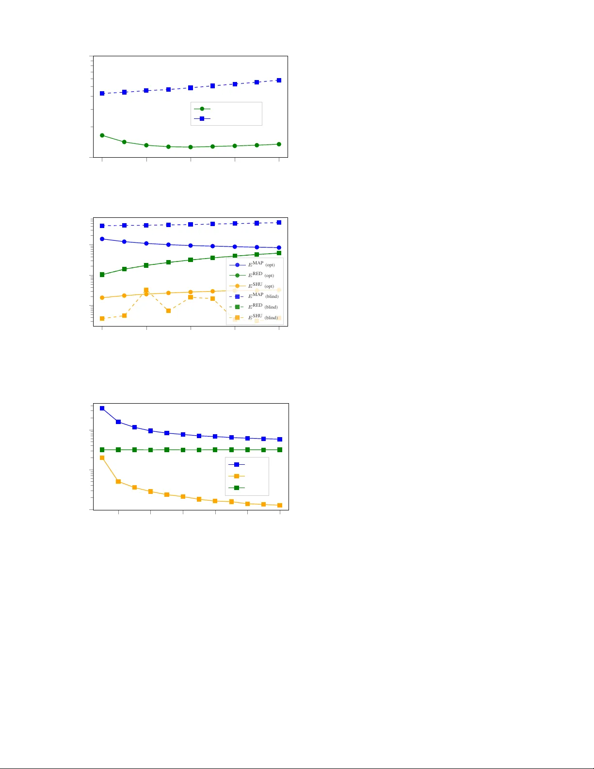
Ener gy-Ef ficient Edge-F acilitated W ireless Collaborati ve Computing using Map-Reduce Antoine Paris, Hamed Mir ghasemi, Ivan Stupia and Luc V andendorpe ICTEAM/ELEN/CoSy , UCLouvain, Louvain-la-Neuv e, Belgium Email: { antoine.paris, seyed.mirghasemi, iv an.stupia, luc.v andendorpe } @uclouvain.be Abstract —In this work, a heter ogeneous set of wireless de vices sharing a common access point collaborates to perform a set of tasks. Using the Map-Reduce distributed computing framework, the tasks are optimally distributed amongst the nodes with the objective of minimizing the total energy consumption of the nodes while satisfying a latency constraint. The derived optimal collaborative-computing scheme takes into account both the computing capabilities of the nodes and the strength of their com- munication links. Numerical simulations illustrate the benefits of the proposed optimal collaborative-computing scheme over a blind collaborative-computing scheme and the non-collaborativ e scenario, both in term of energy sa vings and achievable latency . The proposed optimal scheme also exhibits the interesting feature of allowing to trade energy for latency , and vice versa. Index T erms —wir eless collaborative computing, distributed computing, Map-Reduce, energy-efficiency , fog computing. I . I N T RO D U C T I O N W e consider a set of K nodes, indexed by the letter k ∈ [ K ] , sharing a common access point (AP), base station (BS) or gate way in the context of low-po wer wide-area networks (LPW AN). A node can be any de vice able to wirelessly communicate with the AP and perform local computations. Under a giv en latency constraint τ , each node k wants to compute a certain function φ ( d k , w ) where d k ∈ [0 , 1] D is some D -bit local information av ailable to node k (e.g., sensed information or local state) and w ∈ [0 , 1] L is a L -bit file with L  D bits (e.g., a dataset) that might, for instance, be cached at the AP [1]. In the context of smart cities or smart buildings, w could be the result of the aggregation ov er space and time of information sensed from the en vironment through a network of sensors (e.g., traf fic density or temperature) whereas the nodes could be actuators having some local state d k that periodically need to perform some latency-sensiti ve computations to decide whether to take some actions (e.g., smart traf fic lights or smart thermostats). Other applications include fog computing, mobile crowd-sensing or wireless distributed systems. Owing to the unacceptable delay of mobile cloud computing (MCC), and in the absence of a mobile edge computing (MEC) server nearby , the computing and storage capabilities of wireless devices are limited. It might thus be the case, for example, that w is too large to fit in the memory of a single node, or that the nodes are not individually powerful enough to satisfy the latency constraint. T o overcome those limitations, a collaborativ e-computing scheme based on the Map-Reduce distributed computing framework [2] is proposed. This distributed computing model in volv es local computations at the nodes and communication between the nodes via the AP (i.e., the edge of the network is facilitating the communication between the nodes). In some applications, one could also deliberately avoid the use of a third-party owned MCC or MEC for priv acy reasons. The problem setup and distributed computing model used in this work essentially follo ws [3], with the exceptions that we consider the set of nodes to be heter ogeneous in term of computing capabilities and channel strengths and add an explicit latency constraint. Prior works on wireless distributed computing using Map-Reduce, e.g., [3]–[6], mainly focus on coded distributed computing (CDC) and study the trade-of f between the computation and communication loads incurred by the collaboration. Motiv ated by the fact that wireless devices are often limited in energy and that most computing tasks are accompanied by a latency constraint, this work shifts focus tow ards optimizing the collaborative-computing scheme to minimize the total energy consumption of the nodes, while satisfying the latency constraint. T o our knowledge, this work is the first to incorporate those considerations in a Map-Reduce based wireless collaborative-computing scheme. Throughout this paper , we assume that there is some central entity having perfect knowledge of the channel state information (CSI) and computing capabilities of all the nodes that coordinates the collaboration. Section II starts by describing in details the distributed computing model and the energy and time consumption models for both local computation and communication between the nodes. Next, Sec. III formulates the problem as an optimization problem that turns out to be con vex and to hav e a semi-closed form solution, giv en in Sec. IV. Section V then benchmarks the performances of the optimal collaborative-computing scheme against a blind collaborati ve-computing scheme and the non- collaborativ e scenario through numerical experiments. Finally , Sec. VI discusses the results obtained in this work and opportunities for future research. I I . S Y S T E M M O D E L This section details the distributed computing model used in this work, namely Map-Reduce, and quantifies the time and energy consumed by each phase of the collaboration. A. Distributed computing model The tasks are shared between the K nodes according to the Map-Reduce framework [2]. First, we assume that the file w w AP 1 w 1 2 w 2 · · · K w K { d k } K k =1 { d k } K k =1 { d k } K k =1 g 1 ( d 1 , w 1 ) g 2 ( d 1 , w 2 ) · · · g K ( d 1 , w K ) g 1 ( d 2 , w 1 ) g 2 ( d 2 , w 2 ) · · · g K ( d 2 , w K ) . . . . . . . . . . . . g 1 ( d K , w 1 ) g 2 ( d K , w 2 ) · · · g K ( d K , w K ) 1 Map 2 Map K Map φ ( d 1 , w ) = h ( ) 1 Reduce φ ( d 2 , w ) = h ( ) 2 Reduce φ ( d K , w ) = h ( ) K Reduce Fig. 1. Illustration of the the Map-Reduce distributed computing model. The computation of { φ ( d k , w ) } K k =1 is distributed between K nodes. During the Map phase, each node k computes intermediate values { g k ( d l , w k ) } K l =1 (see framed columns on the above figure). Next, during the Shuffle phase, the intermediate values in bold on the figure are transmitted via the AP to the nodes for which they have been computed. Finally , during the Reduce phase, each node l combines the intermediate values { g k ( d l , w k ) } K k =1 to obtain φ ( d l , w ) (see colored rows on the above figure). can be arbitrarily di vided in K smaller files w k (one for each node) of size l k ∈ R ≥ 0 bits 1 such that w k ∩ w l = ∅ for all k 6 = l and w = S K k =1 w k . W e neglect the time and energy needed to transmit w k from the AP to node k , for all k ∈ [ K ] . T o make collaboration between the nodes possible, we also assume that the local data { d k } K k =1 were shared between all the nodes through the AP in a prior phase that we neglect in this work because D is assumed to be relati vely small. During the first phase of the Map-Reduce framew ork, namely the Map phase , each node k computes intermediate values v k,l = g k ( d l , w k ) , l ∈ [ K ] where g k : [0 , 1] D × [0 , 1] l k → [0 , 1] ( l k /L ) T is the Map function ex ecuted at node k . The size (in bits) of the intermediate values produced at node k is assumed to be proportional to l k . Each node k thus computes intermediate values for all the other nodes (i.e., v k,l for all l 6 = k ) and for itself (i.e., v k,k ) using the part w k of w received from the AP . Next, the nodes exchange intermediate values with each other in the so-called Shuffle phase . More precisely , each node k transmits the intermediate values v k,l = g k ( d l , w k ) to node l via the AP , for all l 6 = k . In total, node k thus needs to transmit ( K − 1)( l k /L ) T bits of intermediate values to the AP . Finally , during the Reduce phase , each node l combines the T bits of intermediate values { v k,l = g k ( d l , w k ) } K k =1 as φ ( d l , w ) = h ( g 1 ( d l , w 1 ) , g 2 ( d l , w 2 ) , . . . , g K ( d l , w K )) where h : [0 , 1] T → [0 , 1] O is the Reduce function . The Map- Reduce distributed computing model is illustrated in Fig. 1. 1 In practice, l k should be an integer multiple of the size of the smallest possible division of w . In this work, we relax this practical consideration to av oid dealing with integer programming later on. Note that l k = 0 is also possible, in which case node k does not participate to the collaboration. B. Local computing model During the Map and the Reduce phases, the nodes hav e to perform some local computations. The local computing model used in this work follows [7]. The number of CPU cycles required to process 1-bit of input data is noted C k while the amount of energy consumed per CPU cycle is noted P k . The amounts of energy consumed at node k during the Map and the Reduce phases 2 are thus given by E MAP k = ( K D + l k ) C k P k and E RED k = T C k P k , (1) respectiv ely . Next, letting F k be the number of CPU cycles per second at node k , the amounts of time required for the Map and the Reduce phases are given by t MAP k = ( K D + l k ) C k /F k and t RED k = T C k /F k , (2) respectiv ely . One can already observe that we can control the energy and time consumed at node k by the Map phase through the variable l k . At the opposite, we don’t hav e any control on the energy and time consumed by the Reduce phase. As a consequence, and because the Map and the Shuffle phases must be over before the Reduce phase can start, the time remaining for the Map and the Shuffle phases is giv en by τ − max k { t RED k } , i.e., the slowest node reduces the av ailable time τ by the amount of time it needs for the Reduce phase. C. Communications fr om the nodes to the AP During the Shuffle phase, nodes exchange intermediate values through the AP. This exchange thus in volv es both an uplink communication (nodes to AP) and a downlink communication (AP to nodes). In most applications howe ver , it is reasonable to assume that the downlink rates are much larger than the uplink rates. For this reason, we neglect the time needed for the downlink communication in this work. W e assume that all the nodes can communicate in an orthogonal manner to the AP (e.g., through frequency division multiple access techniques). W e also make the common assumption that the allowed latency τ is smaller than the channel coherence time. Let h k ∈ C denote the wireless channel from node k to the AP , p k the RF transmit power of node k , B the communication bandwidth, σ 2 the noise po wer at the AP in the bandwidth B , and Γ the SNR gap. The achiev able uplink rate of node k is then giv en by r k ( p k ) = B log 2  1 + p k | h k | 2 Γ σ 2  . The time required by node k to transmit the ( K − 1)( l k /L ) T bits of intermediate v alues to the AP is thus given by t SHU k = αl k /r k ( p k ) where α = ( K − 1) T /L has been de- fined to ease notations. Then, inspired by [7], we define f ( x ) = σ 2 Γ(2 x/B − 1) , and write the energy consumed at node k to transmit the intermediate v alues as E SHU k = p k t SHU k = t SHU k | h k | 2 f  αl k t SHU k  . (3) Through the variables l k and p k (or , equiv alently , t SHU k ), we thus hav e control on the energy and time consumed at node k during the Shuffle phase. 2 Note that we assume that C k and P k are the same for both phases. I I I . P RO B L E M F O R M U L A T I O N As mentioned in the introduction, the objective is to optimize the collaborativ e-computing scheme to minimize the total energy consumption of the nodes, while satisfying the latency constraint τ . This can be mathematically formulated as follo ws minimize { l k } , { t SHU k } P K k =1 E MAP k + E SHU k + E RED k subject to l k , t SHU k ≥ 0 , k ∈ [ K ] t MAP k + t SHU k ≤ τ − max k { t RED k } , k ∈ [ K ] (4) P K k =1 l k = L. (5) Constraint (4) directly follo ws from the discussion at the end of Sec. II-B while (5) ensures that the partition { w k } K k =1 of w fully co vers w . Substituting Eqs. (1) - (3) in the above optimization problem and removing the constant terms from the objective function, we obtain minimize { l k } , { t SHU k } P K k =1 l k C k P k + t SHU k | h k | 2 f  αl k t SHU k  (6) subject to l k , t SHU k ≥ 0 , k ∈ [ K ] l k C k F k + t SHU k ≤ τ k , k ∈ [ K ] (7) P K k =1 l k = L with τ k , the effective latency constraint of node k , giv en by τ k = τ − T max k { C k /F k } − K D C k /F k . (8) This last optimization problem is very similar to the one formulated in [7] and is kno wn to be con ve x [7, Lemma 1]. Next, one can observe that the objecti ve function (6) is always decreasing with t SHU k . Indeed, for a fixed number of bits αl k to transmit during the Shuffle phase, increasing the duration of the transmission t SHU k always decreases the energy consumption E SHU k . As a consequence, constraint (7) is alw ays activ e at the optimum and can thus be turned into an equality constraint 3 . W e can thus get rid of half of the optimization variables by substituting l k by F k C k ( τ k − t SHU k ) . This leads to minimize { t SHU k } P K k =1 ( τ k − t SHU k ) F k P k + t SHU k | h k | 2 f  α F k C k  τ k t SHU k − 1  subject to 0 ≤ t SHU k ≤ τ k , k ∈ [ K ] P K k =1 F k C k ( τ k − t SHU k ) = L. (9) I V . O P T I M A L S O L U T I O N W e start by defining the partial Lagrangian as follows L ( { t k } , λ ) = P K k =1 ( τ k − t k ) F k P k + t k | h k | 2 f  α F k C k  τ k t k − 1  + λ  L − P K k =1 F k C k ( τ k − t k )  3 In the particular case where l k = 0 , the value of t SHU k does not impact the objectiv e function and imposing t SHU k = τ k to make the constraint activ e is thus not an issue. where t SHU k has been replaced by t k to ease notations and with λ the Lagrange multiplier associated to (9) . Then, applying the KKT conditions to the partial Lagrangian leads to ∂ L ∂ t k   ∗ = − F k P k + 1 | h k | 2 f  α F k C k  τ k t ∗ k − 1  − α | h k | 2 F k C k τ k t ∗ k f 0  α F k C k  τ k t ∗ k − 1  + λ ∗ F k C k = − F k P k − Γ σ 2 | h k | 2 + λ ∗ F k C k + Γ σ 2 | h k | 2  1 − α ln(2) B F k C k τ k t ∗ k  2 α B F k C k  τ k t ∗ k − 1       > 0 , t ∗ k = 0 = 0 , t ∗ k ∈ ]0 , τ k ] < 0 , t ∗ k = τ k ⇒ l ∗ k = 0 , with P K k =1 F k C k ( τ k − t ∗ k ) = L. The first case (i.e., > 0 ) can’t happen as the objectiv e goes to + ∞ when t k goes to 0. The last case (i.e., < 0 ) tells us when a node does not participate in the Map and Shuf fle phases (i.e., when l ∗ k = 0 ). It can be re-written as C k P k + α Γ σ 2 | h k | 2 ln(2) B > λ ∗ . (10) The left-hand side of the inequality corresponds to the marginal energy consumption of node k per bit receiv ed, when node k hasn’t receiv ed any bit yet, i.e., at l k = 0 . Indeed, the first term corresponds to the marginal energy consumption incurred by the Map phase while the second term corresponds to the marginal energy consumption incurred by the Shuffle phase. In other words, the left-hand side of (10) can be interpreted as the “price to start collaborating”. If this price is greater than a threshold given by λ ∗ , then l ∗ k = 0 , meaning that node k does not participate to the Map and Shuffle phases 4 . Finally , solving the remaining case (i.e., = 0 ) for t ∗ k leads to t ∗ k = α ln(2) B F k C k × τ k W 0 ( 1 e  | h k | 2 Γ σ 2 F k C k ( λ ∗ − C k P k ) − 1  e α ln(2) B F k C k ) +1 (11) where W 0 ( · ) is the main branch of the Lambert function. The optimization problem can then be solved using a one- dimensional search for λ ∗ , as described in Algorithm 1. Algorithm 1 Binary search for λ ∗ 1: ( λ l , λ h ) = (0 , max k { C k P k + α Γ σ 2 | h 2 k | ln(2) B } ) 2: ( L l , L h ) = ( P k F k C k ( τ k − t ∗ k,l ) , P k F k C k ( τ k − t ∗ k,h )) where t ∗ k,l and t ∗ k,h are obtained using (11) with λ l and λ h , respecti vely . 3: while L l 6 = L and L h 6 = L do 4: L m = P k F k C k ( τ k − t ∗ k,m ) where t ∗ k,m is obtained using (11) with λ m = ( λ l + λ h ) / 2 . 5: if L m > L then , λ h = λ m , compute L h as in step 2. 6: else if L m < L then , λ l = λ m , compute L l as in step 2. 7: else λ ∗ = λ m . 8: end while 4 Note that it still participates to the Reduce phase as it still needs to obtain φ ( d k , w ) . V . N U M E R I C A L R E S U LT S In this section, the performances of the optimal collaborative- computing scheme are benchmarked against a blind collaborati ve-computing scheme and the non-collaborati ve sce- nario through numerical experiments 5 . The blind collaborative- computing scheme simply consists in uniformly distributing w between the K nodes, i.e., l k = L/K , without taking into account their computing capabilities and the strength of their channel to the AP. Unless stated otherwise, the parameters used in the follo wing numerical experiments are giv en in T able I [7]. T ABLE I P A R A M ET E R S U S ED I N T HE N U M ER I C AL E X P ER I M E NT S . Parameter V alue Units C k i.i.d. ∼ Unif ([500 , 1500]) [CPU cycles/bit] P k i.i.d. ∼ Unif ([10 , 200]) [pJ/CPU cycle] F k i.i.d. ∼ Unif ( { 0 . 1 , 0 . 2 , . . . , 1 . 0 } ) [GHz] h k i.i.d. ∼ C N (0 , 10 − 3 ) (Rayleigh fading) / B 15 [kHz] σ 2 1 [nW] Γ 1 / A. Maximum computation load and outage probability W e start by looking at the maximum computation load (i.e., the maximum size of w ) that can be processed by the different schemes under a giv en latency constraint. F or both the optimal and the blind collaborative-computing schemes, the maximum computation load is achieved when τ k , the effecti ve latency , is entirely used to perform local computation, that is, when an infinite amount of energy is used for the Shuffling phase and t SHU k → 0 . The maximum computation load of the optimal and blind collaborative-computing schemes are thus given by L opt max = P K k =1 F k C k τ k and L blind max = K min k n F k C k τ k o , respectiv ely . For the case where the nodes do not collaborate (i.e., each node is working for itself only), the maximum computation load that can be processed in the allowed latency τ is giv en by L solo max = min k n F k C k  τ − D C k F k o . If we consider the computing capabilities of the nodes as random variables, L ∗ max can also be considered as a random v ariable. Thus, for a giv en computation load L , one can define the outage probability P ∗ out of the system as follows P ∗ out = P [ L ∗ max < L ] . Figure 2 shows the empirical outage probability of the dif ferent schemes as a function of the allowed latency τ for se veral numbers of nodes K . This figure illustrates one of the adv antage 5 Source code available at https://github.com/anpar/EE- WCC- MapReduce. Clicking on a figure will directly lead you to the code that generated it. 0 . 5 1 1 . 5 2 2 . 5 10 − 4 10 − 3 10 − 2 10 − 1 10 0 Allowed latency τ [s] Outage probability P ∗ out K = 10 (opt) K = 20 (opt) K = 30 (opt) K = 40 (opt) K = 10 (blind) K = 20 (blind) K = 30 (blind) K = 40 (blind) K = 10 (solo) Fig. 2. Empirical outage probability for the optimal collaborative-computing scheme (opt), the blind collaborative-computing scheme (blind) and the non- collaborativ e scenario (solo). Each data point is the result of an average on 1M experiments with L = 4Mb, D = 100b and T = 5kb. of the optimal scheme: for a giv en number of nodes K and a giv en allo wed latency τ , this is the scheme with the highest probability of satisfying the latency constraint. Increasing the number of nodes is also more profitable with the optimal scheme than it is with the blind scheme. This is because the optimal scheme lev erages diversity amongst the nodes, while the blind scheme, as suggested by its name, is blind to that div ersity and considers all the nodes as being equals. B. Energy consumption and energy-latency trade-off Figure 3a compares the total energy consumption of the nodes when using the optimal and the blind scheme. Each point on the figure is the result of an average over 10000 random feasible (for both the optimal and the blind schemes) instances of the problem, with L = 4Mb, D = 100b, T = 5kb and with the allowed latency τ set to 1 s to ensure feasibility by both schemes with relativ ely high probability . This figure shows that the optimal scheme consumes approximately four to five times less energy than the blind scheme. Note that the total energy consumed in the non-collaborativ e scenario can easily be shown to be roughly K times larger than the total energy consumed by the blind scheme. Next, Fig. 3b breaks do wn the total ener gy consumptions of both the optimal and the blind schemes into three components associated to the different phases of the collaboration, i.e., E MAP , E SHU and E RED . First of all, this figure shows that most of the energy is consumed by the Map and Reduce phases 6 . Next, and at the opposite of the blind scheme, the optimal scheme is able to reduce E MAP when K increases, again by leveraging div ersity amongst the nodes. This explains the slow decrease of the total energy consumption with K visible on Fig. 3a. At some point howe ver , the unav oidable energy consumption of the Reduce phase starts to gro w faster than E MAP decreases and the total energy consumption rises again. Finally , Fig. 3c depicts how the different energy components of the optimal 6 Note that this result depends a lot on the value of the parameters presented in T able I and should thus not be interpreted as a general result. 20 40 60 80 100 10 − 1 10 0 Number of nodes K T otal ener gy consumption [J] Optimal scheme Blind scheme (a) Comparison of the total energy consumed by the optimal and the blind scheme for τ = 1 s . 20 40 60 80 100 10 − 3 10 − 2 10 − 1 Number of nodes K Energy consumption [J] E MAP (opt) E RED (opt) E SHU (opt) E MAP (blind) E RED (blind) E SHU (blind) (b) Breakdown of the energy consumed by the three phases of the collaboration, both for the optimal (opt) and the blind (blind) collaborative computing scheme, for τ = 1 s . Note that the energy consumption for the Reduce phase is the same in both case. 0 . 5 1 1 . 5 2 2 . 5 3 10 − 3 10 − 2 10 − 1 Allowed latency τ [s] Energy consumption [J] E MAP E SHU E RED (c) Evolution of the energy consumed by the three phases of the optimal collaborativ e-computing scheme, as a function of the latency , for K = 60 . Fig. 3. Energy consumption of the nodes when L = 4Mb, D = 100b and T = 5kb . Each point is the result of an average over 10000 feasible (for each scheme) instances of the problem. scheme ev olve with the allo wed latency τ . In particular , this figure shows that the optimal scheme is able to decrease the energy consumed by the Map phase when τ increases. This is again a benefit of the div ersity amongst the nodes: increasing the allowed latency allows the optimal scheme to use slo wer but more energy-ef ficient nodes, hence decreasing the energy consumption. V I . D I S C U S S I O N A N D F U T U R E W O R K S In this work, an energy-ef ficient wireless collaborati ve- computing scheme inspired by the Map-Reduce framework has been proposed. Numerical experiments highlighted the benefits of this scheme over a blind scheme and the non- collaborati ve scenario: lower achiev able latency , reduced energy consumption and the ability to trade energy for latency and vice versa. Those benefits are obtained by lev eraging the diversity of the nodes in term of computing capabilities and channel strength. Analytical results highlighting the benefits of div ersity are howe ver missing and their pursuit thus constitutes a first possible direction for future works. A second obvious direction for future works might be to refine the optimization problem formulated in Sec. III to account for additional constraints, e.g., limited memory capacity , maximum RF transmit power or limited battery lev el. Next, the models used in this work to quantify the time and energy consumed by the different phases of the collab- oration are very simple and far from being realistic (see, for instance, [8]). Incorporating more realistic models in the proposed collaborative-computing scheme will thus certainly be a priority in future works. Finally , as opposed to the original Map-Reduce framew ork that considers some redundancy between the smaller files { w k } K k =1 to increase the robustness of the system to node failure and to prior works [3]–[6] that study the trade- off between computation and communication load through network coding, we did not assume an y redundancy in this work. Inv estigating the possible benefits of redundancy in the proposed scheme is thus another interesting research question. A C K N O W L E D G M E N T AP is a Research Fellow of the F. R . S . - F N R S. This work was also supported by F. R . S . - F N R S under the E O S program (project 30452698, “MUlti-SErvice WIreless NET work”). R E F E R E N C E S [1] D. Liu, B. Chen, C. Y ang, and A. F . Molisch, “Caching at the wireless edge: design aspects, challenges, and future directions, ” IEEE Communications Magazine , vol. 54, no. 9, pp. 22–28, Sep. 2016. [2] J. Dean and S. Ghema wat, “Mapreduce: Simplified data processing on large clusters, ” in OSDI’04: Sixth Symposium on Operating System Design and Implementation , San Francisco, CA, 2004, pp. 137–150. [3] S. Li, Q. Y u, M. A. Maddah-Ali, and A. S. A vestimehr , “ A scalable framew ork for wireless distributed computing, ” IEEE/ACM T ransactions on Networking , vol. 25, no. 5, pp. 2643–2654, Oct 2017. [4] M. Kiamari, C. W ang, and A. S. A vestimehr , “Coding for edge-facilitated wireless distributed computing with heterogeneous users, ” in 2017 51st Asilomar Confer ence on Signals, Systems, and Computers , Oct 2017, pp. 536–540. [5] S. Li, M. A. Maddah-Ali, Q. Y u, and A. S. A vestimehr , “ A fundamental tradeoff between computation and communication in distributed com- puting, ” IEEE T ransactions on Information Theory , vol. 64, no. 1, pp. 109–128, Jan 2018. [6] F . Li, J. Chen, and Z. W ang, “W ireless MapReduce Distributed Computing, ” 2018. [Online]. A vailable: http://arxiv .org/abs/1802.00894 [7] C. Y ou, K. Huang, H. Chae, and B. Kim, “Energy-efficient resource allocation for mobile-edge computation offloading, ” IEEE T ransactions on W ir eless Communications , vol. 16, no. 3, pp. 1397–1411, March 2017. [8] T . Bouguera, J.-F . Diouris, J.-J. Chaillout, R. Jaouadi, and G. Andrieux, “Energy consumption model for sensor nodes based on lora and lorawan, ” Sensors , vol. 18, no. 7, p. 2104, 2018.