Centroid-based deep metric learning for speaker recognition

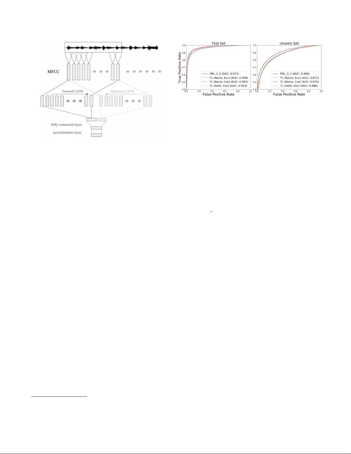
CENTR OID-B ASED DEEP METRIC LEARNING FOR SPEAKER RECOGNITION Jixuan W ang 1 , 2 , K uan-Chieh W ang 1 , 2 , Mar c T . Law 1 , 2 , F rank Rudzicz 1 , 2 , 3 , 4 , Michael Brudno 1 , 2 , 5 1 Uni versity of T oronto, Canada 2 V ector Institute, Canada 3 St Michaels Hospital, Canada 4 Surgical Safety T echnologies Inc, Canada 5 Hospital for Sick Children, Canada { jixuan, wangkua1, la w , frank, brudno } @cs.toronto.edu ABSTRA CT Speaker embedding models that utilize neural networks to map utterances to a space where distances reflect similarity between speakers hav e driv en recent progress in the speaker recognition task. Howe ver , there is still a significant perfor - mance gap between recognizing speakers in the training set and unseen speakers. The latter case corresponds to the few- shot learning task, where a trained model is e valuated on un- seen classes. Here, we optimize a speak er embedding model with prototypical network loss (PNL), a state-of-the-art ap- proach for the few-shot image classification task. The result- ing embedding model outperforms the state-of-the-art triplet loss based models in both speaker verification and identifica- tion tasks, for both seen and unseen speakers. Index T erms — deep metric learning, triplet loss, se- quence embedding, speaker recognition 1. INTR ODUCTION The dev elopment of embedding models to represent speech features in high-dimensional space has enabled elegant solu- tions to speaker recognition problems, including speaker ver - ification (SV), and speaker identification (SI). Speaker verifi- cation systems verify whether or not a given utterance comes from some claimed speaker , while only having access to a handful of enrolled utterances (i.e. training examples). In the speaker identification task, a trained model is asked to classify among K speakers gi ven small amount of enrollment speech. For both tasks, finding good representation of speech features is essential to recognition of the speaker , especially with small training sets: the variation in phrases needs to be normalized, while variation across speak ers must be preserved. T raditional pipelines that combine i-vector and proba- bilistic linear discriminant analysis (PLD A) separately train the feature extractor and the final classifier [1]. Howe ver , performance of i-vector systems drops for short speech ut- terances [2]. More robust feature extractors have been pro- posed, including replacing i-vectors with features extracted from deep networks [3, 4]. Most recent efforts hav e relied The first two authors contributed equally to this w ork. (a) prototypical network loss (b) triplet loss Fig. 1 : Comparison between the effect of prototypical net- work loss (PNL) and triplet loss (TL) on the embedding. Dashed lines represent distances encouraged to increase, while solid lines represent distances being decreased. left : For PNL, prototypes for different speakers, denoted by black nodes are computed as the mean of the support set (shaded) during training. right : For TL, a triplet consists of an anchor , positiv e, and ne gati ve samples, forming the (anchor , positi ve) and (anchor,ne gativ e) pairs. Depending on the sampling strat- egy not all triplets may be considered. on optimizing an end-to-end deep model with the triplet loss (TL) [5, 6, 7, 8] and the generalized end-to-end (GE2E) loss [9] to build the speak er embeddings . In this paper we propose the use of prototypical network loss (PNL) to opti mize an end-to-end speak er embedding net- work. PNL was introduced for the few-shot image classifica- tion task [10] and is the state-of-the-art approach on sev eral few-shot learning benchmarks. Howe ver , to the best of our knowledge, PNL has not been applied to speaker embedding or related problems. Here we show that for SV and SI tasks, a model trained with PNL outperforms an embedding network of the same architecture optimized with TL. W e discuss why PNL is a better formulation for learning an embedding model and provide empirical observ ations as to why it might be eas- ier to use in practice. 2. RELA TED WORK Speaker embedding networks: In traditional i-vector based methods for speaker embedding, a universal background model is first b uilt. Then, a PLD A model is trained to mea- sure the similarity of i-v ectors. Replacing traditional i-vectors with speaker embedding models based on deep neural net- works has lead to improvement in SV [4, 3]. Nonetheless, a PLD A classifier is still needed to compare the similarity of embeddings. More recently , end-to-end training of an em- bedding network that makes decision by comparing distance in the embedding to a cross-validated threshold outperformed traditional methods. For detailed comparison between em- bedding networks and i-vector based methods, we refer the reader to [6, 4, 3]. Building on top of these studies, our work focuses on the comparison between two different approaches for deep metric learning (TL [5, 6, 7, 8] and PNL [10]) for end-to-end speaker embedding models. Deep metric learning: End-to-end speaker embedding models can be seen as a form of deep metric learning, which has been widely studied in the machine learning literature. Early examples of metric learning with neural networks in- clude signature [11] and f ace verification [12]. Both compare pairs of examples with standard similarity functions (e.g. co- sine or Euclidean distance) at the final embedding layer of a siamese architecture. More complex loss functions inv olving triplets { anchor , positive , ne gative } were later proposed [13], and shown to perform well on f ace verification [14]. Few-shot learning: Motiv ated by the fact that humans can learn new concepts from only a handful of examples, researchers have proposed the challenging task of “few-shot learning” [15, 16]. The test-time task is to classify examples among K new classes (i.e. unseen during training) while only being giv en a handful of labeled examples from these new classes. The same consideration arises naturally for speaker recognition tasks, as speakers encountered during test time may be different. It is essential to build profiles for previ- ously unseen speakers with limited data. In contrast to previ- ous applications of PNL [10], we use it in conjunction with a recurrent neural network for sequential data (i.e. speech) rather than a con volutional netw ork for images. 3. OPTIMIZA TION SCHEMES & MODEL W e now explain the standard triplet loss scheme and compare it to PNL [10]. W e then describe the model we optimize using the two schemes for speaker embedding. 3.1. T riplet loss For triplet-based models, we denote by S 0 = { x 1 , · · · , x N 0 } the examples in one mini-batch of size N 0 , where x i is a sequence of speech features. These models sample triplets, which consist of an anchor x a , a positive sample x p with the same speak er label, and a negati ve sample x n with a dif ferent speaker label. For each triplet τ = ( x a , x p , x n ) , the triplet loss is formulated as: L ( τ ) = max (0 , d a,p − d a,n + α ) (1) where d a,b = d ( f ( x a ) , f ( x b )) , d and f are the distance func- tion (e.g. cosine or squared Euclidean distance) and speaker embedding model, respectively , and α > 0 is a margin. Min- imizing L ( x a , x p , x n ) learns representations so that the sim- ilar pair ( x a , x p ) has smaller distance than the dissimilar pair ( x a , x n ) , adjusted by the mar gin. It is worth noting that the triplet loss does not minimize distances between similar pairs (i.e., when d a,p − d a,n + α < 0 ); it only tries to preserve some order between distances. Finally , the loss for a mini- batch is J T L = P τ ∈ T L ( τ ) where T is the set all of pos- sible triplets in the mini-batch. In the conte xt of v ery large datasets, creating all the possible triplets is computationally expensi ve; dif ferent triplet sampling strate gies ha ve been pro- posed to ensure fast conv ergence while av oiding de generate solutions. For instance, the semi-hard mining strategy [14] samples only one hard neg ativ e pair for each positive pair . A triplet is “hard” if d a,p − d a,n + α > 0 . 3.2. Prototypical Netw orks Loss Prototypical Networks [10] train a neural network episodi- cally; each episode is composed of one mini-batch contain- ing K categories (here, speakers). The mini-batch contains a support set called S and a query set called Q . In our case, the support set S = { ( x i , y i ) } N i =1 represents each e xample as a sequence of speech feature vectors x i with corresponding speaker label y i ∈ { 1 , · · · , K } . W e denote S k ⊆ S as the set of examples in S of speaker k . The prototype (or centroid) of each class c k ∈ R M is calculated as the mean of embeddings in the support set: c k = 1 | S k | X ( x i ,y i ) ∈ S k f ( x i ) (2) where f is the speaker embedding model which maps se- quences of speech features into the M -dimensional embed- ding space (see details in Section 3.3). During training, each query example { ( x j , y j ) } ∈ Q is classified against K speakers based on a softmax over dis- tances to each speaker prototypes: p ( y = y j | x j ) = exp  − d ( f ( x j ) , c y j )  Σ k 0 exp ( − d ( f ( x j ) , c k 0 ) (3) where d is the distance function. The loss function for each mini-batch is J P N L = P { ( x j ,y j ) }∈ Q − log p ( y = y j | x j ) 3.3. Speech sequence embedding model In terms of network architecture, we use the same speech sequence embedding model as T ristouNet [7]. W e use the same model architecture when optimizing with each of the two losses above. As shown in Fig. 2, the sequence of Mel-frequency cepstral coefficients (MFCC) features are col- lected. They are then fed into bidirectional LSTM [17]. The outputs from the forward and backward LSTMs are first av erage-pooled over time, concatenated, then processed by a fully connected layer and a normalization layer . Fig. 2 : Speech sequence embedding model 4. EXPERIMENT In this section, we introduce the experiments conducted for ev aluation and comparison of different models. 4.1. Datasets and implementation details W e use the VCTK corpus [18] and a subset of V oxCeleb2 dataset [8]. VCTK corpus contains clearly read speech, while V oxCeleb2 has more background noise and ov erlap- ping speech. Speech data of the first 90 speakers in VCTK corpus was divided into training, v alidation and test sets. Data of the remaining 18 speakers was used as an “unseen” set to ev aluate the generalizability of the method. For V oxCeleb2, we selected a subset containing 101 speakers (we refer to this subset as V oxCeleb2 dataset for conciseness) and use data of 71 speakers for training and validation, while the other 30 speakers are used as the “unseen” set. W e use the default implementation of TristouNet for fea- ture extraction and speech sequence embedding models. In the following, we refer to the models by the loss used dur- ing optimization (i.e. PNL vs. TL) as the architecture of the embedding network is fixed. Featur e extraction W e extracted 19-dimensional MFCCs, their first and second deri vati ves, along with the first and sec- ond deri vati ves of energy in a 25ms window e very 10ms using the pyannote multimedia processing toolkit 1 and Y aafe toolkit [19]. This results in 59-dimensional acoustic features. W e use 2-second segments for both PNL and TL models to ensure comparability of results and to test performance on shorter utterances. T raining W e use PyT orch [20] for implementation of both losses 2 . The output dimension is 16, and the tanh acti v ation 1 http://pyannote.github .io/ 2 Our implementation of PNL is based on that of the original authors: https://github .com/jakesnell/prototypical-networks [10] Fig. 3 : “ same/differ ent ” experiments on test and unseen sets. function is used for the fully connected layer . Squared Eu- clidean distance is used as the distance function. The mar- gin α used in our implementation of TL is 0 . 2 following [7]. For both models, the Adam optimizer [21] is used with 10 − 3 learning rate. Both models are trained for 100 epochs. For each mini-batch, we randomly choose 15 speakers without replacement on VCTK (10 speakers on V oxCeleb2). W e enforce equal mini-batch size between the two formula- tions (i.e., | S | + | Q | = N 0 ). TL models are trained with Eu- clidian distance or cosine distance using na ¨ ıve or semi-hard strategy . PNL models are trained with different size of sup- port and query sets. T o a void confusion in the follo wing, “TL ( s , d )” denotes sampling strategy s with distance metric d , and “PNL ( x y , d )” denotes PNL using x -shot with query set of size y training episodes. 4.2. “ Same/Diff erent ” experiments As with TristouNet [7], we first conduct “ same/differ ent ” e x- periments on the VCTK corpus. The same number of posi- tiv e (same speak er) and negati ve (different speakers) pairs are randomly selected. For each pair of segments, we calculate the distance between their embeddings and compare it with a threshold to predict whether they are from the same or dif fer- ent speakers. W e report the recei ver operating characteristic (R OC) curve for each model, shown in Fig. 3. All models perform comparably well on seen data set. Howe ver , on the unseen data PNL model outperforms TL models. 4.3. Speaker Identification T o ev aluate SI performance, we simulate each test task with a batch of K speakers, each with S enrollment samples, and Q query samples. Classification of a query is done by finding the closest prototype based on some metric d . Results are shown in T able 1, from which one can observe that the 3-shot PNL- based model outperforms the TL (Semi, Euc) model on all tasks, especially on the more challenging 18-way SI task (6% and 19% relativ e improvement on test and unseen data set, respectiv ely). Interestingly , the one-shot PNL based model performs better than triplet loss based model with na ¨ ıve sam- pling strategy while it “sees” many fewer positive and nega- tiv e pairs for each batch. It also performs nearly as well as TL that uses the more complicated semi-hard sampling strategy . T able 1 : SI accuracy on test and unseen sets of VCTK. Under the Model column are the training configurations. The top row ‘S: N S , Q: N Q , K -way’ denotes the task configurations. Model S: 5, Q: 5, 6-way S: 10, Q: 10, 18-way T est Unseen T est Unseen TL (Naiv e, Euc) 91.96% 77.80% 81.25% 56.37% TL (Naiv e, Cos) 92.37% 77.69% 83.51% 58.51% TL (Semi, Euc) 93.33% 79.69% 85.38% 58.49% TL (Semi, Cos) 92.13% 73.94% 83.99% 52.97% PNL (1 5, Euc) 93.24% 77.90% 83.71% 56.52% PNL (3 5, Euc) 95.63% 84.81% 90.53% 69.64% PNL (5 5, Euc) 95.47% 83.69% 89.85% 68.55% PNL (10 10, Euc) 94.38% 85.00% 88.43% 66.63% T able 2 : SI accuracy on V oxCeleb2. Model 15-way S: 10, Q: - S: 30, Q: - T est Unseen T est Unseen TL (Semi, Cos) 74.74% 53.92% 75.18% 59.61% TL (Semi, Euc) 71.78% 51.74% 72.02% 56.79% PNL (5 5, Euc) 78.38% 59.44% 79.23% 66.63% T able 3 : EER of SV on both data sets. “2s” (2 seconds) refers the duration of speech we used for enrollment. (a) EER on VCTK Model T est Unseen 60s 60s 10s TL (Semi, Cos) 5.43( ± 0.16) 13.87( ± 0.37) 16.19( ± 0.86) TL (Semi, Euc) 5.05( ± 0.09) 12.26( ± 0.69) 13.44( ± 0.91) PNL (5 5, Euc) 4.08( ± 0.13) 10.77( ± 0.58) 12.00( ± 0.76) (b) EER on V oxCeleb2 Model T est Unseen 60s 60s 10s TL (Semi, Cos) 9.23( ± 0.13) 14.62( ± 0.35) 16.93( ± 0.45) TL (Semi, Euc) 9.90( ± 0.11) 15.92( ± 0.32) 17.61( ± 0.51) PNL (5 5, Euc) 8.29( ± 0.12) 13.68( ± 0.26) 15.67( ± 0.56) 4.4. Speaker verification T o ev aluate SV performance, we randomly select some speech segments for enrollment. Then, 200 (resp. 100) segments of each speaker are selected as positive samples on V oxCeleb2 (resp. VCTK). Equal number of negati ve sam- ples are selected from different speakers. During enrollment phase, speaker prototypes are computed from the enrollment set. For verification, the decision is made by comparing the distance between the embedding of the query segment and the speaker prototype to a threshold. Performance is ev aluated by equal error rate (EER). Results are shown in T able 3. Results obtained by repeating the experiments 10 times (i.e. mean and standard deviation) on VCTK and V oxCeleb2 are shown in T able 3a and T able 3b, respectiv ely . EER of PNL model is significantly lower than that of TL models ( p  0 . 001 using t-test) across all tasks. As expected, both models perform reasonably well on test set of VCTK, while a little worse on test set of V oxCeleb2. For unseen set, EERs of all models decrease for longer duration of speech data for enroll- ment. Although TL (Semi, Cos) outperforms TL (Semi, Euc) on more noisy data set, PNL still achiev es the lo west EER. 4.5. Analysis The fact that generalization improv es as the number of data points per category increases for the PNL model may be ex- plained by the fact that PNL is a specific (supervised) formu- lation of clustering with Bregman div ergences [22]. The pro- totype of each category approximates the point that minimizes the loss in Bregman information [22] for that category . Breg- man information is related to Shannon’ s rate distortion theory , it corresponds to the optimal distortion-rate to encode a cat- egory when the distortion is measured by d (i.e., the squared Euclidean distance). The point that minimizes the loss in Bregman information [22] for the cate gory is the mean v ector of all the examples that belongs to the category . Therefore, the larger the number of ‘shots’, the better the approximation of the mean v ector of the examples in the category . Ho wev er , a larger number of shots does not necessarily lead to better performance as discussed in [10]. Statistical guarantees of (a generalization of) PNL are studied in [23]. In practice, PNL is quite robust to the choice of number of shots. W e find that anywhere between 3 to 10 shots work well. The reason why SI accuracy of TL models drops dramati- cally for experiments with more “ways” might be due to lim- itation of TL, which has been extensi vely studied in the lit- erature in different contexts [24, 25]. One main limitation is that TL does not necessarily group each cate gory into a single cluster ev en when the global optimum is reached [24]. In our experience, PNL is practically easier to use than TL. PNL is not dependent on a triplet sampling strategy , that can impact performance, and do not require the margin pa- rameter α . PNL models are also ∼ 3x faster to train (wallclock time) than TL models with same mini-batch size because TL requires more pairwise comparisons for batches of same size. 5. CONCLUSION W e hav e proposed a prototypical network loss-based speaker embedding model, and compared it with the popular triplet loss-based models. With identical speech sequence embed- ding architectures, PNL outperforms the triplet loss when speakers are seen during training, and by an e ven larger margin on held-out, unseen speakers for both speaker iden- tification and speaker verification tasks. W e also illustrate some of the practical adv antages of PNL models ov er TL. In the future, we would like to explore better architectures of speech sequence embedding models and integrate the fe w- shot learning based speaker embedding model into a speaker diarization pipeline. 6. REFERENCES [1] Najim Dehak, Patrick J Kenn y , R ´ eda Dehak, Pierre Du- mouchel, and Pierre Ouellet, “Front-end factor analysis for speaker verification, ” IEEE T ransactions on Audio, Speech, and Language Pr ocessing , vol. 19, no. 4, pp. 788–798, 2011. [2] Achintya Kumar Sarkar , Driss Matrouf, Pierre Michel Bousquet, and Jean-Franc ¸ ois Bonastre, “Study of the effect of i-vector modeling on short and mismatch utter - ance duration for speaker verification, ” in Interspeech , 2012. [3] Da vid Sn yder , Daniel Garcia-Romero, Gre gory Sell, Daniel Po ve y , and Sanjee v Khudanpur , “X-vectors: Ro- bust dnn embeddings for speaker recognition, ” Submit- ted to ICASSP , 2018. [4] Da vid Snyder , Daniel Garcia-Romero, Daniel Pove y , and Sanjeev Khudanpur, “Deep neural network em- beddings for text-independent speaker verification, ” in Pr oc. Interspeech , 2017, pp. 999–1003. [5] Chao Li, Xiaokong Ma, Bing Jiang, Xiangang Li, Xuewei Zhang, Xiao Liu, Y ing Cao, Ajay Kannan, and Zhenyao Zhu, “Deep speaker: an end-to-end neural speaker embedding system, ” arXiv pr eprint arXiv:1705.02304 , 2017. [6] Chunlei Zhang and Kazuhito K oishida, “End-to-end text-independent speaker verification with triplet loss on short utterances, ” in Pr oc. of Interspeech , 2017. [7] Herv ´ e Bredin, “Tristounet: triplet loss for speaker turn embedding, ” in ICASSP . IEEE, 2017, pp. 5430–5434. [8] Joon Son Chung, Arsha Nagrani, and Andrew Zisser- man, “V oxceleb2: Deep speaker recognition, ” arXiv pr eprint arXiv:1806.05622 , 2018. [9] Li W an, Quan W ang, Alan Papir , and Ignacio Lopez Moreno, “Generalized end-to-end loss for speaker verification, ” in 2018 IEEE International Conference on Acoustics, Speech and Signal Pr ocessing (ICASSP) . IEEE, 2018, pp. 4879–4883. [10] Jake Snell, K evin Swersky , and Richard Zemel, “Proto- typical networks for fe w-shot learning, ” in NIPS , 2017. [11] Jane Bromley , Isabelle Guyon, Y ann LeCun, Eduard S ¨ ackinger , and Roopak Shah, “Signature verification using a” siamese” time delay neural network, ” in NIPS , 1994. [12] Sumit Chopra, Raia Hadsell, and Y ann LeCun, “Learn- ing a similarity metric discriminati vely , with application to face verification, ” in CVPR , 2005. [13] Matthe w Schultz and Thorsten Joachims, “Learning a distance metric from relative comparisons, ” in NIPS , 2004. [14] Florian Schroff, Dmitry Kalenichenko, and James Philbin, “Facenet: A unified embedding for face recog- nition and clustering, ” in CVPR , 2015. [15] Li Fei-Fei, Rob Fergus, and Pietro Perona, “One-shot learning of object categories, ” IEEE TP AMI , vol. 28, no. 4, pp. 594–611, 2006. [16] Brenden M Lake, Ruslan Salakhutdinov , and Joshua B T enenbaum, “Human-lev el concept learning through probabilistic program induction, ” Science , vol. 350, no. 6266, pp. 1332–1338, 2015. [17] Sepp Hochreiter and J ¨ urgen Schmidhuber , “Long short- term memory , ” Neural computation , vol. 9, no. 8, pp. 1735–1780, 1997. [18] Christophe V eaux, Junichi Y amagishi, Kirsten MacDon- ald, et al., “Superseded-cstr vctk corpus: English multi- speaker corpus for cstr v oice cloning toolkit, ” 2016. [19] Benoit Mathieu, Slim Essid, Thomas Fillon, Jacques Prado, and Ga ¨ el Richard, “Y aafe, an easy to use and efficient audio feature extraction software., ” in ISMIR , 2010, pp. 441–446. [20] Adam Paszke, Sam Gross, Soumith Chintala, Gregory Chanan, Edward Y ang, Zachary DeV ito, Zeming Lin, Alban Desmaison, Luca Antiga, and Adam Lerer, “ Au- tomatic differentiation in p ytorch, ” in NIPS-W , 2017. [21] Diederik P Kingma and Jimmy Ba, “ Adam: A method for stochastic optimization, ” arXiv preprint arXiv:1412.6980 , 2014. [22] Arindam Banerjee, Srujana Merugu, Inderjit S Dhillon, and Joydeep Ghosh, “Clustering with bregman diver - gences, ” JMLR , vol. 6, no. Oct, pp. 1705–1749, 2005. [23] Marc T Law , Jake Snell, Amir massoud Farahmand, Raquel Urtasun, and Richard S Zemel, “Dimensionality reduction for representing the kno wledge of probabilis- tic models, ” in ICLR , 2019. [24] Hyun Oh Song, Stefanie Jegelka, V ivek Rathod, and Ke vin Murphy , “Deep metric learning via facility lo- cation, ” in CVPR , 2017. [25] Marc T . Law , Nicolas Thome, and Matthieu Cord, “Learning a distance metric from relativ e comparisons between quadruplets of images, ” IJCV , pp. 65–94, 2017.