Deep Learning for Vertex Reconstruction of Neutrino-Nucleus Interaction Events with Combined Energy and Time Data

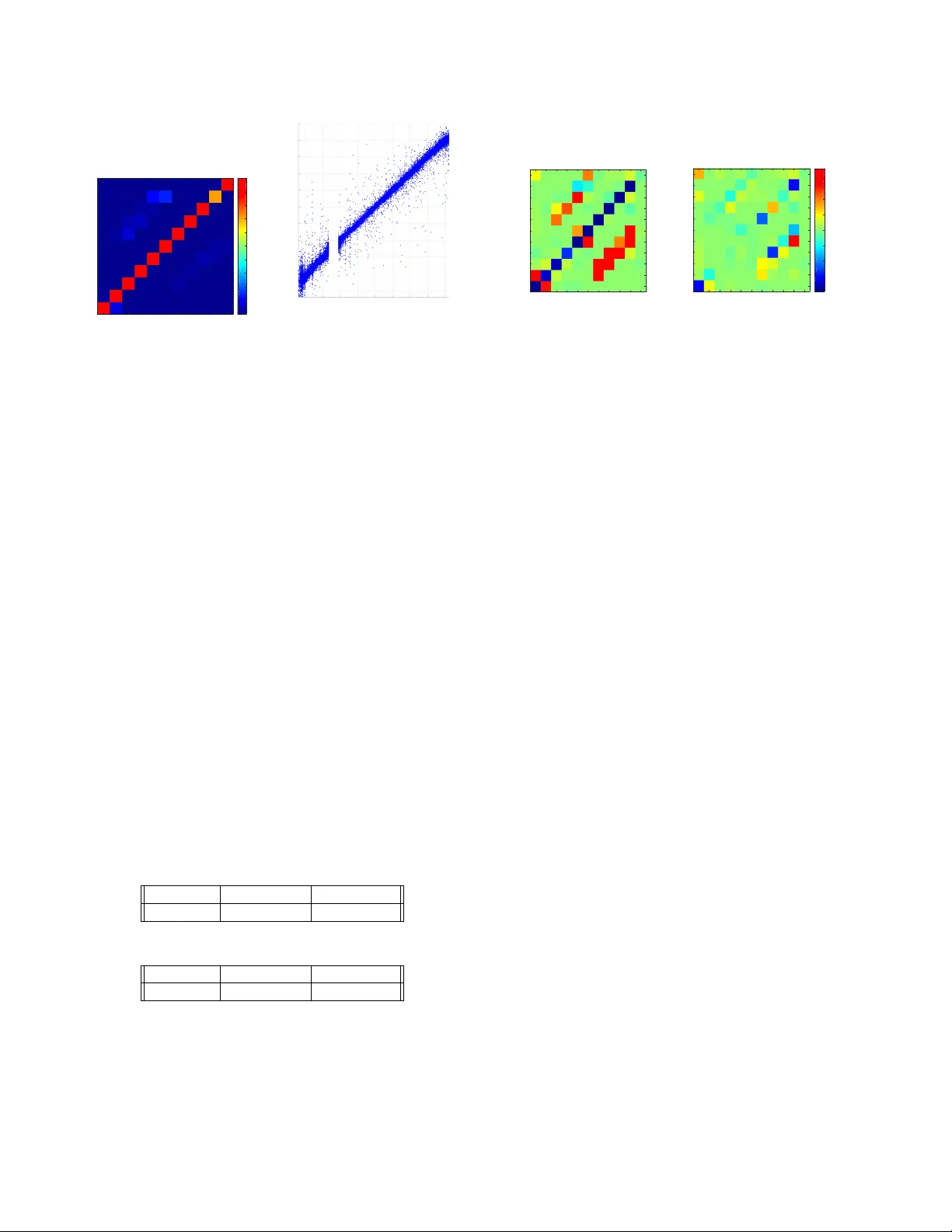
DEEP LEARNING FOR VER TEX RECONSTR UCTION OF NEUTRINO-NUCLEUS INTERA CTION EVENTS WITH COMBINED ENERGY AND TIME D A T A Linghao Song † , F an Chen † , Steven R. Y oung ‡ , Catherine D. Schuman ‡ , Gabriel P er due ⊥ , and Thomas E. P otok ‡ † Duke Uni versity , Durham, North Carolina, 27708 ‡ Oak Ridge National Laboratory , Oak Ridge, T ennessee, 37831 ⊥ Fermi National Accelerator Laboratory , Batavia, Illinois, 60510 ABSTRA CT W e present a deep learning approach for verte x reconstruc- tion of neutrino-nucleus interaction events, a problem in the domain of high ener gy physics. In this approach, we combine both energy and timing data that are collected in the MIN- ERvA detector to perform classification and regression tasks. W e show that the resulting network achie ves higher accuracy than previous results while requiring a smaller model size and less training time. In particular , the proposed model outper- forms the state-of-the-art by 4.00% on classification accuracy . For the regression task, our model achiev es 0.9919 on the coefficient of determination, higher than the previous work (0.96). Index T erms — V ertex reconstruction, high ener gy physics, con volutional neural networks, deep learning 1. INTR ODUCTION MINERvA (Main Injuector Experiment for v-A) [1] is a leading-edge program at Fermi National Accelerator Labora- tory . The primary focus of the MINERvA experiment is to understand neutrino properties and reactions. Neutrinos are subatomic particles that rarely interact with normal matter as they only interact via weak subatomic force and gravity and they hav e e xtremely small mass. The study of neutrinos may help physicists understand the matter-antimatter imbalance in the universe [2]. Howe ver , understanding their interac- tions with nuclear matter poses significant challenges: they probe aspects of nuclear structure that are not accessible with electrons, photons, or protons [3]. In the MINERvA experiment, the detector is exposed to the Neutrinos at the Main Injector (NuMI) neutrino beam [4]. The detector records both energy and timing information that Notice: This manuscript has been authored by UT -Battelle, LLC under contract DE-AC05-00OR22725, and Fermi Research Alliance, LLC (FRA) under contract DE-A C02-07CH11359 with the US Department of Energy (DOE). The US government retains and the publisher, by accepting the arti- cle for publication, acknowledges that the US gov ernment retains a nonex- clusiv e, paid-up, irrevocable, worldwide license to publish or reproduce the published form of this manuscript, or allow others to do so, for US gov ern- ment purposes. DOE will provide public access to these results of federally sponsored research in accordance with the DOE Public Access Plan ( http: //energy.gov/downloads/doe- public- access- plan ). can be used to determine where neutrino-nucleus interaction ev ents occur . Precise determination of the interaction vertex, also known as vertex reconstruction [5], is required to identify the target nucleus in MINERvA. Segment T arg et Beam Direction (+Z) 0 1 10 9 8 7 6 5 4 3 2 1 5 4 3 2 W ater T arg et U/X V /X Active Scintilla tor Modules Passive T argets Fig. 1 . Simple illustration of the MINERvA detector . Fig.1 illustrates a simple detector layout. W e eliminate details of the detector and the physics measurements ob- tained, b ut readers can refer to [1, 5] for details. The core of the detector consists of a series of alternating active and passiv e target regions along the beam direction. The passive targets are solid layers of dif ferent materials or their combi- nations, e.g., carbon, iron, lead, and tanks of liquid helium and water . Note in the datasets considered in this work, the liquid/water tar get is empty . The activ e targets are plastic scintillator (a hydrocarbon) modules. Each activ e module contains a pair of planes with scintillator strips aligned in one of three orientations: X, U or V . Strips in X planes are ori- ented v ertically and U and V strips are oriented ± 60 ◦ relativ e to X. Each module contains either a U or V plane, follo wed by an X, such that the pattern is interleav ed UXVXUXVX, etc. Ener gy and timing values collected from the detector are mapped to pixel values in an image, which can be used for subsequently verte x reconstruction. A key issue associated with data from this experiment and scientific data in general is that it is often extremely dif ficult to obtain labels. For example, there may be only a hand- ful of experts in the world capable of labeling experimental data effecti vely , and even then, it may be impossible to es- tablish ground-truth labels for the data that multiple experts will agree is correct. As such, much of the scientific data that can be used for training is generated using simulations. For this study , millions of simulated neutrino-nucleus scattering ev ents were created and represented as images. In this case, deep learning approaches to analyze the data can help physi- cists in quickly interpreting results from the experiments. The contributions of this work are: (1) the incorporation of both energy and time lattices in one network to boost clas- sification accuracy , (2) the utilization of transfer learning to improv e performance on regression of absolute position, and (3) a new network topology to combine three views (X, U, V) and reduce model size. 2. D A T A DESCRIPTION The dataset used for training, v alidation and testing consisted of 1 , 453 , 884 simulated ev ents. Neutrino-nucleus interac- tions were simulated using the GENIE Neutrino Monte Carlo Generator [6], and the propagation of the resulting radiation through the bulk detector was simulated using the Geant4 toolkit [7]. For each e vent, there is both an ener gy lattice and a time lattice, each of which consists of three views: an X-view , a U-vie w , and a V -view . The i mages from the X-view are 127 × 94 pixels, while the others (U-view and V -view) are 127 × 47 pixels. Each pixel in the energy lattice giv es informa- tion about the a verage energy value ov er the detection ev ent at that point, while each pixel in the time lattice recorded the timing information in nanoseconds relati ve to when the inter - action is predicted to occur . energy-x strip time-x plane energy-u time-u plane energy 0 5 10 15 20 25 30 35 40 energy-v -40 -20 0 20 40 times time-v plane strip Fig. 2 . Example of the neutrino interaction e vents. There are three scales at which we can attempt to predict the vertex location. The largest scale is a segment. The de- tector can be split into 11 segments, each of which consists of multiple planes within the detector . Approaching a smaller scale, the detector can be split into each of the planes. Planes are thin, horizontally stacked bundles of activ e sensors. They are oriented roughly perpendicular to the neutrino beam. Fi- nally , the vertex location can be defined as the absolute mea- sured position (Z) inside the detector . 3. PREVIOUS WORKS The initial approach to verte x reconstruction for this dataset was to identify linear tracks and calculated the intersection points of multiple tracks as the vertex. This method fails for certain types of ev ents; in particular, it is dif ficult to identify verte x when tracks are non-linear or differentiate individual tracks when the number of track is great. A previous work has applied deep learning (specifically conv olutional neural networks) to the ener gy lattice of the data (as images) to im- prov e classification accuracy [5]. Another pre vious work has applied spiking neural networks to the v ertex reconstruction problem using the time lattice only [8], achie ving comparable results to the conv olutional approach for a single vie w of the data, which indicated that the timing data includes informa- tion rele vant to the vertex reconstruction problem as well. It is worth noting that both of these approaches utilize an older version of the dataset that used a reduce input size as com- pared with the dataset used here. Another work explored the use of Domain Adversarial Neural Networks [9] for control- ling physics modeling bias [10]. In this work, we seek to com- bine both the ener gy lattice and time lattice in a con volutional neural netw ork implementation. The neural network model is designed to predict the segment and absolute position (Z) of the neutrino ev ents. 4. APPR OA CH 4.1. Model for Segment Classification T o get a network with smaller size and to alleviate the vanishing-gradient problem, inspired by the ResNet [11] and DenseNet [12], we designed our network for segment classification as shown in Fig.3(a). A rectangle represents a series of operations. For ex- ample, a rectangle labeled as B,C,P means that batch nor- malization (B), con volution (C) and max pooling (P) are successiv ely applied to the input tensors. All con volutions (C) in the network are configured with kernel size=3 , padding=1 and stride=1 , and a ReLU activ ation func- tion is applied. The kernel size and stride for the max pooling (P) is 2. The octagon below a rectangle indicates the output tensor size, while an octagon on the flow indicates the con- catenated tensor size or the reformed tensor size. The tensor size format is C, H , W , where C is the number of channels, H is the height and W is the width. F or example, the input tensor e,t(u,v,x) has 2 groups (energy and timing) of 3 views (U, V , X), thus 6 channels of 127-by-94 matrix. A black dot indicates the concatenation of two tensors by channel. There are three blocks (B1, B2 and B3) in the net- work. W ithin each block, the input of each rectangle is a con- B,C,P (24,63,47) (6,127,94)  B,C (24,63,47) (48,63,47) B,C (24,63,47) (48,63,47) B,C,P (24,31,23) C2 (48,31,23) (24,31,23) B,C (24,31,23) (48,31,23) B,C (24,31,23) (48,31,23) B,C,P (24,15,11) C4 (24,15,11) C2 (24,15,11) (72,15,11) B,C (24,15,11) (48,15,11) B,C (24,15,11) (48,15,11) B,C,P (24,7,5) fc (11) classification (840) B1 B2 B3 (a) Classification model (840) fc (512) fc (1) regr ession From CONV layers (b) Regression model Fig. 3 . The networks for (a) segment classification and (b) Z regression. In the Z regression, the con volutional layers in the trained classification network were frozen, and two fully-connected layers were added and retrained. catenation of two tensors: the output of a previous rectangle and a shortcut identical tensor . For each block, we also ap- ply direct-connect from previous blocks. F or block B2, the direct-connect is a conv olution (C2) with a kernel size and stride of 2. So, the input for B2 is the concatenation of two (24,31,23)-tensors, i.e., a tensor of size (48,31,23). For block B3, two direct-connects (C2 and C4) are used. C4 is a con vo- lution with kernel size and stride of 4. Thus, the input tensor size for block B3 is (72,15,11). Note that there is no activ a- tion function for the conv olutions of the three direct-connects. For the final classification layer , we reformed the output ten- sor (24,7,5) to a tensor (840), and a fully-connected layer is employed. 4.2. Model for Z Regr ession Because we use the same data for Z-regression as we do for segment classification, it is quite natural to employ a trans- fer learning approach. Fig.3(b) sho ws the model used for Z regression. W e use a well trained segment classification net- work, freeze all the con volutional layers, and add two fully- connected layers (840-512-1) for regression. 5. EXPERIMENTS 5.1. Experimentation Details For the whole dataset ( 1 , 453 , 884 ev ents), W e separated this set into three parts, 1 / 9 for testing, 1 / 9 for validation, and 7 / 9 for training. Each data sample contains three vie ws (X, U, V) for timing and energy , i.e., a total of six views. The size of data for the X view is 127 × 94 while the size for U and V views is 127 × 47 . W e repeated the U and V views on the second axis to get a size of 127 × 94 . Then, we concate- nate the six 127 × 94 views to a obtain a tensor (6,127,94) as an input. The original data was in a float32 format. W e first normalized the data by view and con verted the data to uint8 format for fast training access. W e also calculated the mean ( µ ) and standard de viation ( σ ) on the training set, and applied whitening on input data; thus, the mean and standard deviation for all vie ws are 0 and 1 respecti vely . In the training of the classification network, we use an SGD optimizer . The training takes 20 epochs. The learning rate is 0.1 for the first 10 epochs, 0.01 for the follo wing 5 epochs and 0.001 for the last 5 epochs. SGD is configured with a momentum of 0.8 and a weight decay of 5e-4, and the batch size is 256. Then we trained the regression network for 8 epochs with a learning rate of 0.001. T w o NVIDIA TIT AN X (Pascal) GPUs are configured in data parallelism for train- ing. The toolkit used is PyT orch. 5.2. Overall Results with Both Energy and T iming Data T able 1 . Comparison to previous w ork [5] [5]* This W ork Image Size 127 × 50 127 × 94 127 × 94 Accuracy 94.09% 88.97% 98.09% R 2 0.96 0.8886 0.9919 Model Size 14.5MB - 0.488 MB T raining Time 10 hrs - 2.5hrs *These results were created by re-implementing the network from a previous w ork [5], and ev aluating against updated dataset. W e compare our work with a previous work [5] in T able 1. For the segmentation classification, our model (shown in Fig.3(a)) achiev es an accurac y of 98.09% on testing dataset, 4.00% higher than that in [5]. For the Z regression, the co- efficient of determination ( R 2 ) of our model (as shown in Fig.3(b)) is 0.9919, higher than the previous work (0.96). Ad- ditionally , the model size (the size of the trained model file) and the training time of our model are smaller than those of [5]. Fig.4(a) sho ws the heatmap of the confusion matrix of the segment classification with both energy and timing data. W e can see our model performs well for almost all segments ex- cept Segment 9. W e e xpect that this is due to the imbalance of the training data, in which only 0.47% of the data is labeled as Segment 9. W e show the scatter plot of the predicted Z of 1 2 3 4 5 6 7 8 9 10 11 1 2 3 4 5 6 7 8 9 10 11 0 0.1 0.2 0.3 0.4 0.5 0.6 0.7 0.8 0.9 1 10 9 8 7 6 5 4 3 2 1 0 0 1 2 3 4 5 6 7 8 9 10 1.0 0.9 0.8 0.7 0.6 0.5 0.4 0.3 0.2 0.1 0.0 1 2 3 4 5 6 7 8 9 10 11 1 2 3 4 5 6 7 8 9 10 11 0 0.1 0.2 0.3 0.4 0.5 0.6 0.7 0.8 0.9 1 (a) Confusion matrix 9000 8500 8000 7500 7000 6500 6000 5500 5000 4500 4000 4500 5000 5500 6000 6500 7000 7500 8000 8500 T rue Z (mm) Predicted Z (mm) (b) Scatter plot Fig. 4 . (a) Heatmap of confusion matrix of the segment clas- sification and (b) scatter plot of the predicted and true Z (mm) on testing dataset with both energy and timing data. The wa- ter target(no detector) is around 5250mm, so there is a gap. our regression model with both timing and energy data and true Z in Fig.4(b). The standard deviation σ of the difference of the predicted Z and the true Z is 115.61 mm. 5.3. Classification and Regression with Only Timing Data and Only Energy Data While we have both timing and energy data, we are also in- terested in classification and regression with only timing or energy data. In pre vious work [5], only energy data was used. For segment classification with only timing or energy data, we use the same network as shown in Fig.3(a), where the input is a tensor of X, U, V views of timing or energy data, b ut not both simultaneously as in the previous section. Thus, the input tensor size is (3, 127, 94). T able 2 shows the segment classification accuracy of our model when both timing and energy data were used (combined) and when only timing or ener gy data was used. As sho wn in this table, when only timing or energy data was used, the accuracy is slightly degraded. Howe ver , it is clear that the ener gy data contrib uted more as the accurac y when only energy data was used is only 0.13% less than when both types of data are used. T able 2 . Segment classification accuracy on testing dataset Combined Only T iming Only Energy 98.09% 96.92% 97.95% T able 3 . Regression R 2 on testing dataset Combined Only T iming Only Energy 0.9919 0.9915 0.9901 T o get more details about the performance of the model when only timing or energy data is used, we show the heat map of the dif ference of the confusion matrix when only tim- ing or energy data was used, compared that when both were used in Fig.5. A warmer color square on the diagonal is bet- ter , while a warmer color square at other position than on the diagonal means misclassification. Again, we find that energy data contributes more in the se gment classification. 1 2 3 4 5 6 7 8 9 10 11 1 2 3 4 5 6 7 8 9 10 11 -0.02 -0.015 -0.01 -0.005 0 0.005 0.01 0.015 0.02 10 9 8 7 6 5 4 3 2 1 0 0 1 2 3 4 5 6 7 8 10 9 (a) Only timing data 1 2 3 4 5 6 7 8 9 10 11 1 2 3 4 5 6 7 8 9 10 11 -0.02 -0.015 -0.01 -0.005 0 0.005 0.01 0.015 0.02 10 9 8 7 6 5 4 3 2 1 0 0 1 2 3 4 5 6 7 8 10 9 .020 .015 .010 .005 0.00 -.005 -.010 -.015 -.020 (b) Only energy data Fig. 5 . Heatmap of the difference of confusion matrix of clas- sifications on testing dataset with (a) only timing data and (b) only energy data compared to that when both timing and en- ergy data were used. Finally , we also compare the Z re gression when only tim- ing or energy data was used as sho wn in T able 3. While the R 2 for the three scenarios are almost the same, but for a more accurate Z regression, both timing and energy data should be used. 6. CONCLUSION In this work we present a deep learning approach for vertex reconstruction in neutrino interaction data. W e demonstrate state-of-the-art results on this task, presenting a model that achiev es higher accuracy on the dataset while also reducing both the training time required as well as the model size. For future work, we plan to explore the utilization of recurrent neural networks for capturing spatial-temporal features from within the ev ent timing. Acknowledgements This material is based upon work supported by the U.S. Department of Energy , Office of Science, Of fice of Advanced Scientific Computing Research, Robinson Pino, program manager , under contract number DE-A C05-00OR22725. W e would like to thank the MINERvA collaboration for the use of their simulated data and for many useful and stim- ulating con versations. MINERvA is supported by the Fermi National Accelerator Laboratory under US Department of Energy contract No. DE-A C02-07CH11359 which included the MINERvA construction project. MINERvA construc- tion support was also granted by the United States National Science Foundation under A ward PHY -0619727 and by the Univ ersity of Rochester . Support for participating MIN- ERvA physicists was provided by NSF and DOE (USA), by CAPES and CNPq (Brazil), by CoNaCyT (Mexico), by CON- ICYT (Chile), by CONCYTEC, DGI-PUCP and IDI/IGIUNI (Peru), and by Latin American Center for Physics (CLAF). This research was supported in part by an appointment to the Oak Ridge National Laboratory ASTR O Program, spon- sored by the U.S. Department of Energy and administered by the Oak Ridge Institute for Science and Education. 7. REFERENCES [1] L. Aliaga, L. Bagby , B. Baldin, A. Baumbaugh, A. Bodek, R. Bradford, W .K. Brooks, D. Boehnlein, S. Boyd, H. Budd, et al., “Design, calibration, and per- formance of the minerv a detector , ” Nuclear Instruments and Methods in Physics Researc h Section A: Acceler- ators, Spectr ometers, Detectors and Associated Equip- ment , vol. 743, pp. 130 – 159, 2014. [2] R Acciarri, MA Acero, M Adamowski, C Adams, P Adamson, S Adhikari, Z Ahmad, CH Albright, T Alion, E Amador , et al., “Long-Baseline Neutrino Facility (LBNF) and Deep Underground Neutrino Ex- periment (DUNE) Conceptual Design Report, V olume 4 The DUNE Detectors at LBNF, ” ArXiv e-prints , p. arXiv:1601.02984, Jan. 2016. [3] Ulrich Mosel, “Neutrino Interactions with Nucleons and Nuclei: Importance for Long-Baseline Experiments, ” Ann. Rev . Nucl. P art. Sci. , vol. 66, pp. 171–195, 2016. [4] P Adamson, K Anderson, M Andrews, R Andre ws, I Anghel, D Augustine, A Aurisano, S A vvakumov , DS A yres, B Baller , et al., “The numi neutrino beam, ” Nuclear Instruments and Methods in Physics Resear ch Section A: Accelerators, Spectrometer s, Detectors and Associated Equipment , vol. 806, pp. 279–306, 2016. [5] Adam M T erwilliger, Gabriel N Perdue, David Isele, Robert M Patton, and Stev en R Y oung, “V ertex recon- struction of neutrino interactions using deep learning, ” in Neural Networks (IJCNN), 2017 International J oint Confer ence on . IEEE, 2017, pp. 2275–2281. [6] Costas Andreopoulos, Christopher Barry , Stev e Dyt- man, Hugh Gallagher, T omasz Golan, Robert Hatcher, Gabriel Perdue, and Julia Y arba, “The genie neutrino monte carlo generator: Physics and user manual, ” arXiv pr eprint arXiv:1510.05494 , 2015. [7] Sea Agostinelli, John Allison, K al Amako, John Apos- tolakis, H Araujo, P Arce, M Asai, D Axen, S Banerjee, G 2 Barrand, et al., “Geant4-a simulation toolkit, ” Nu- clear instruments and methods in physics r esear ch sec- tion A: Accelerators, Spectr ometers, Detectors and As- sociated Equipment , v ol. 506, no. 3, pp. 250–303, 2003. [8] Catherine D Schuman, Thomas E Potok, Ste ven Y oung, Robert Patton, Gabriel Perdue, Gangotree Chakma, Austin W yer, and Garrett S Rose, “Neuromorphic com- puting for temporal scientific data classification, ” in Pr oceedings of the Neur omorphic Computing Sympo- sium . A CM, 2017, p. 2. [9] Y aroslav Ganin, Evgeniya Ustinova, Hana Ajakan, Pas- cal Germain, Hugo Larochelle, Franc ¸ ois Laviolette, Mario Marchand, and V ictor Lempitsky , “Domain- adversarial training of neural networks, ” J. Mach. Learn. Res. , vol. 17, no. 1, pp. 2096–2030, Jan. 2016. [10] GN Perdue, A Ghosh, M W ospakrik, F Akbar, DA An- drade, M Ascencio, L Bellantoni, A Bercellie, M Be- tancourt, GFR Caceres V era, et al., “Reducing model bias in a deep learning classifier using domain adversar - ial neural networks in the minerv a experiment, ” Journal of Instrumentation , vol. 13, no. 11, pp. P11020, 2018. [11] Kaiming He, Xiangyu Zhang, Shaoqing Ren, and Jian Sun, “Deep residual learning for image recognition, ” in Pr oceedings of the IEEE confer ence on computer vision and pattern r ecognition , 2016, pp. 770–778. [12] Gao Huang, Zhuang Liu, Laurens v an der Maaten, and Kilian Q W einber ger, “Densely connected con volutional networks, ” in 2017 IEEE Confer ence on Computer V i- sion and P attern Recognition (CVPR) . IEEE, 2017, pp. 2261–2269.