Detecting the Trend in Musical Taste over the Decade -- A Novel Feature Extraction Algorithm to Classify Musical Content with Simple Features

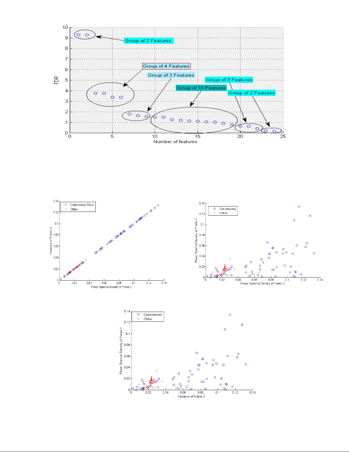
Detecting the T rend in Mus ical Taste ov er the Decade – A Novel Featur e Extraction A lgorithm to Classify Mus ical Content with Simple Features Anish Achary a 1 1 Dept. of Electr ical E ngineering a nd Com puter Science Henry Sam ueli School of Enginee ring University of Cali fornia-Irvine Abstract: This work proposes a novel feature selection algorithm to classify Songs into differe nt groups. Classification of musical content is often a non-trivial job and still relatively less explored area. The main idea conve ye d in t his article is to come u p with a new feature selection scheme that doe s the classification job elegantly and with high accurac y but with simpler but wisely chosen small number of features thus being less prone to over-fitting. This uses a ver y basic gener al idea about the structure of the audio signal which is generally in the shape of a trapezium. So, using thi s general ide a of the Musical Comm unity we propose three frames to be considered and anal yzed for feature extraction for each o f the audio si gn al - opening, stanzas and closing and it has been established with the help of a lot of experiments that this scheme leads to much efficient classification with less complex features in a low dimensional feature space thus is also a computationally less exp ensive method. Step by step anal ysis of feature ex traction, feature ranking, dim ensionality reduction using PCA has been carried in this article. Sequential Forward s election (SFS) algorithm is used to explore the most s ignificant features both with the raw Fisher Discrimi nant Ratio (FDR) and also with the significant eigen-values after PCA. Also during classification extensive validation and cross validation has been don e in a mont e -carlo manner to ensure validity of the claims. 1. Introduct ion: For the past few decades audio processing and classification of songs has emerged as an important and interesting field of stud y. Wit h increasing volum e of data being cr eated in the musi c industry it is often very use ful to de velop powerful and efficient classification algorithms to classif y Music files into different classes of int erest. I n most of the real world problems we face, we hardl y get a precise symbolic representation of a son g and on e has to deal with only th e aud io samples obtained from the sampling of the exact waveform. However, these audio samples can’t be used directl y in AI applic ation algorithms because of the low level and low density of information contained within them [1]. The first step to deal wit h this in an AI problem would be to extra ct me aningful features from the audio samples to get adequate information and emplo y further processing. After the features a re ex tracted the idea is to select the most efficient and meaningful feature rather th an to take all the features in account keeping in mind the case of over-fitti ng. Thus the idea is to extract meaningful f eatures from the audio signals, then to rank them according to some pre -defined criterion and s elect the independent and most significant features [2]. All the music Classification tasks performed previously uses complex features like timbre f eatures such as temporal features, energ y fe atures, spectral shape fe atures, perceptual features; melod y/ harmony features such as pitch function, unfolded or fold ed function; rh y thm features such as tempo, musical patterns etc. And, of cou rse these complex features are n ecessary as it is extremely difficult to analyze musical content and classif y them into different classes using simple statisti cal features like moments, entropy, spectral density etc. However, the m ajor contribution of this article is to claim that such simple features can also be used to give good classification accurac y if chosen wisel y . Thus this paper pro poses the idea of segmenting the audio file into thr ee most significa nt frames namely Opening, S tanzas and Closing and then extracting sim ple statis tical features like different moments, Power Spectral Densit y, Fano-Factor etc f rom each of these frames. Extensive experiments are presented to claim the validity o f this claim. One thumb rule of any P attern recognition problem is to not only choose the features but to choose the most effective one and keeping the number of features to minimal number. There is more than one reason to reduce the number of feature to a sufficient minimum. Features with high correlation coefficient between them, if treated separately in creases the complex ity without much gain in information. A large number of features are directly translated to a large number of classifier par ameters thus might lead to over-fitting. Thus for a finite a nd usually limited number of training patterns keepin g the number of features as small as possi ble is in line with our goal of designing classifiers with good generalization capabilities [3]. Thus after extracting the features the most important question is to reduce the dimension of feature space in such that minimal information is lost. Thus as a first step to do so S tatistical h y pothesis testing and deviation bounds are invoked to eliminate less informative featu res i.e. easily recognizable ‘bad’ choices at the very beginning. Now, eliminating f eatures b y lookin g at them is far from optimal and hen ce as the next step in Feature Selection more elaborate techniques of feature ranking lookin g at th eir interdependen ce are investigated. In this paper Fisher Discriminant Ratio (FDR) has been us ed as the rankin g criterion of the features [4], [5]. Also, Principal Component Anal ysis (PCA) has also been investigated to select features le ading to largest principal components thus leading to minimal information loss in the proc ess of dimension ality reduction. Here in this work a thorough investigation of feature selecti on has been taken care of to ensure selection of best features as well as removal of r edundant or dependent fe atures. Th e class ical method of Sequential Forward Selection (SFS) scheme has been used for t hat purpose. The same idea of Sequential Forward Selection (SFS) al gorithm has been used in case of PCA based f eature selection and all the results have been reported. Indian Musi c has alw ays been considered as one of the richest and most complex to ana lyze with so many delicate and complex variants ranging from Hard Rock, Contemporar y Rock, Pure Classical, Semi Classical and so man y more variants and thus it is very difficult to draw a line between two as the genres are not well defined and has a lot of overlap. Thu s even a binar y classification of Indian Music is a non - trivial task and that too on the basis of simple statistical features li ke moments gives ve ry low accuracy. However, it has been shown here that with the help of the proposed Frame Selection and Feature extraction procedure claimed highl y accurate results are possible even in lo w dimensional Feature Space using simple c lassical s tatistical Featu res like moments, Fano Factor, S pectral Density etc. On the process o f exploring Indian Music two major observations are also drawn. Firstl y, the statis tical difference of so called Indian Rock music with I ndian Classical music and Secondly, the evolution of Indian Hit Music over the last decade i.e. it has been shown that Indian hit music of the 90’s era is statistically dif ferentiable with the nature of hit music of 2000 era. Thus this can be extended to conclude that the musical taste of the Indian Music audience has also changed over the last decade. The classification of Indian Music between two different decades whi ch leads to an intuit ion of the musical taste change of the I ndian Music audienc e with good accuracy is as difficult as it sounds. The me re fact that one would expect high overlap between the musi c of tw o decades and thus the songs might not be easily separable into two distinct classes and thus it is a non -trivial problem. However, with the proposed scheme seems to achieve good results even in case of such difficult problem. Finding the best Classifier for the proposed scheme is also very crucial. Thus, ex tensive experiment has been done with different Classifiers and their corresponding accuracies have been reported. As a first exploration of the proposed scheme the anal y sis has been only restricted to Supervised Learning. However, exploration of Clustering Algorithm performances and r equired modifications of the scheme will be very interesting and left as a f uture work. The main Classifiers used here are- Linear Discriminant Analysis (LDA), Quadratic Discriminant Analysis (QDA), Naïve Bayes, LDA with Moholanbish distance, k - Nearest Neighborhood (KNN) with different criterions to select the k nearest neighbors viz . Euclidian distance, Ci t y block (sum of absolut e difference), Cosine similarity, correlation based; Support Vector Machine (SVM) with linear kernel, quadratic kernel, Rbf k ernel, pol ynomial kernel each with three differ ent methods to ca lculate the separating h yper-plane n amely- Quadratic programming (QP), Sequential Minimal Optimization (SMO) and Least S quares (LS). Each of the classification tasks have been done us ing 500 fold cross validation in Monte-Carlo manner to ensure good generalization of the results. The rest of the paper is organized as follows: In Section 2 we propose our two claims - Firstly, we talk about the chosen dataset which itself is unique and was poorl y understood before. Also, we propos e our algorithm of p artitioning each song alon g with all in tricate details which is our main claim. In section 3 we talk about feature ex traction proc edures along with the pre-processing steps and giving an ove rview of the chosen features a nd the rationale behind choosing th em. Section 4 gives a brief ov erview on Feature selection sche mes in the li ghts of Hypothesis te sting devi ation bounds, along with the implementation detail and re sults. In section 5 we talk about differe nt feature ranking algorithms, especially those used in this paper and also provide implementation det ail of our chosen algorithm. After gaining det ailed knowledge about the Statistics of musi c we shift to Machine Learning regime in the next section. This section talks about different commonl y used supervised learning techniques and also talks about the chosen cl assifiers alon g with implementation detail and extensive experimental results. Section 7 concludes and summarizes our findings in the paper and also gives some intuition about the future line of work on the problem. The Reference section provides a thorough citation o f all the relevant work. 2. Introduction to the D ataset and propo sing a no vel Feature Extr action schem e: In the regime of Music processing it is quite common to extract statistical features that are too complicated and not straight forward statistical measures. The y also rely on tags like artist name, song title etc. For example Million Song Dataset [9] a very commonly used quite popular dataset in the Music Information Retrieval Comm unity provides man y features like song t it le, artist name, artist term frequency, track ID et c which might be useful in building recommender s ystems based on collaborative filtering however does n ot tell much about the statistics of the music and we believe that Music does not have any geographical or language boundary and can be classified only through statistical anal ysis of the music signal. The statistical fe atures used here are not straight forward a nd mostl y complex or hybrid features for example timber, pitch, loudness, tem po etc which are f ine in case of musical sense ho wever they don’t generalize to basic statistical features. They also use some loos ely defined features like artist hotness, dance -ability, bea t confidence, son g hotness etc which ac cording to us cannot be a good indicator of musical content. O ne might conclude a nd it is quite natural th at it is tremendousl y diff icult to analyze musical content only in terms of stand ard statistical features lik e standard moments, sp ectral density et c is very dif ficult and these statistical features are not often significant and do not have good discrimination power. Thus now we can understand from the outset th at classif y ing music based on simple statisti cal features only is not simple and often prove to be insi gnificant. However, this article proposes a new f eature extraction scheme which has been proved to increase the dis crimination power of these simple statistical features and thus this pa per claims that if prope rly chosen then even these simple statistical features can lead to ex cellent classification results as have been proven with extensive experiments in subsequent parts of this paper. The main idea is based on a simple fact, well kn own but often ignored in Musi c Inf ormation Retrieval and have never been exploited before in an y literature regarding Musical Information Retrieval before. It is well known in the Musical Community that t he time domain waveform of an y song falls into the envelope of a tr apezium. Thus, if we look at the time domain amplitude enve lope of a song it shoul d lo ok like a trapezium called Trapezoidal envelope and has been reported in various literatures [6] [7] and the waveform looks like as shown in Fig.1.and has three main distinguish able part namel y – Opening/ Attack, Stanzas/ Sustain, Closing/Decay. The same notion is known as Mukhra, Alap and Antara in Indian Music. So, the proposal is to select three zones of a music signal ac cording to this noti on and treat each Frame as individual entities. The main intuition behind this is that instead of analyzing the entire musi c signal as a whole it is more reasonable to look into these three frames as it is more li kely that these three frames will provide better intuition about the statistics of the son g. Thus, inst ead of extraction statistical features from the entire s ong we rather extract features from each of these fr ames and treat them as new features so though our feature space increases three folds but still intuitively we are more li kely to ex tract more information and even simple features like moments of a particular frame might prove to be and is e xpected to captur e more information an d turn out to be of h igher discriminating power. Indian Music is considered as one of the richest and versatile in the world with so man y variants w hich range from purel y C lassical to Rock however if we look into the current genre classification of Indian music there is no existing genre classification wh ich can suc cessfully classify Indian music in different categories. The main reason behind that mi ght be the fact that Indian Musi c tends to be too compl ex to be classified and as a result it’s like fusion of commonl y claimed genres like Rock, pop, jazz, hip -hop etc statistically. Though the y sound entirely different but if we look deeply into the statistics of Indian Music a proper classification even into two separate classes is a non-trivial task as ever ything seems overlapping with the dist inction in mannerism of the song whi ch can be v ery difficult to understan d in terms of simple statistic al features. Thus, as we claim our alg orithm is strong enough to c lassify Complex and highl y ove rlapping Music like Indian Music and also take the opportunity to be the fi rst to perform such tasks on Indian music to categorize int o two classes - Old Indian music (1985-1999) and Contemporary I ndian Music (2000-2014) and we have chosen around 350 Samples from both the category to anal y ze. All these songs used in thi s paper are chosen blindly f rom the Popular R atings available in various Mu sic Ranking W ebsites p urely bas ed on popularity. This serves two purposes- Firstly, as can b e understood that it is very difficult to classify any kind of music based on era’s and thus these broad classes are expected to have significant overlap and may not b e easily separable and h ence it would serve as a g ood platform to test our claim of increa sing separability of fe atures if chosen accordingly. Secondl y , this would be the first attempt to classify the Hit Music of two de cades and from that we might be able to conclude on how the tast e of the audience have changed ov er the past decade. Thus this can also be extended to infer about the trend change in Musical Taste over time. Thus all sa id and done the first step is to verify whether the assumpti on of music files having a trapezoidal envelope was true. For that one song from each categor y is randomly chosen and the time domain amplitude plots are verified to be supportive of the rationale behind the proposal as can be seen from Fig.2 and Fig.3 and can be re adily verified to indeed resemble with the trapezoidal envelope shown in Fig.1. F ig.1. Trapezoi dal Env elope Fig.2. Music of 90s resembles Trapezoidal envelop e Fig .3. Contempora ry Music audio e nvelope Thus looking at the two signal envelopes of the t ime signal of both t ype of music it c an be concluded that both resemble the general pattern of the trapezoidal envelope as shown in fi g. 1. However, a close look reveals that each frame of a son g belonging to a particular class sig nificantly dif fers from the corresponding frame of the audio belon ging to th e other class. Thus as it has been claimed in this paper that dividing each audio file into these three frames and ex tracting f eatures from them separately looks to be reasonable. Thus in order to proceed with this new promising idea to divide int o these thre e frames it is very important to comment on the size of each fra me. It is ver y clear that intuitivel y it is very difficult to propose an accurate exac t length of each frame as the duration of each frame might var y from one song to another . Thus to pin point a particular bound ary between one fra me to another for all songs is not possible. Howev er, it c an be seen that intuitivel y th e first 4 -6% belong to Frame 1 and last 4-6% approximately belong to Frame 3. Thus, after a few ex periments it seems to work best if the First 5% of the samples are considered to belong to F rame 1 i.e. openin g and the last 5% belonging to closing o r Frame 3. Thus, for the r est of the paper the frame siz es are unanimously distributed as- Frame1 is the first 5% samples of the audio signal, Frame 2 is the next 90% of the audio signal and last 5% o f the samples belong to Frame3 as the generalized division rule for all the audio files. 3. Feature Extraction and D ataset Cre ation: “Not for too smart people who loves complex features and complex algorithms” a motivating quote found in the well known Machine Learning book by Bishop et. al. [ 8] provides the motivation to keep things simple if possible. This is exactly the back bone of the paper. Th e idea is to establish that if chosen in the proposed manner ev en simple statistical features can lead to good s eparability. Thus, eight most common statistica l character istics have bee n taken into account viz. Mean, Variance, Skewness, Kurtosis, Hyper-skewness, Hyper-flatness, Fano-Factor and Power S pectral Density. Ea ch characteristic has been investigated for 3 mentioned frames leading to 24 Features. And the f eatures are named as Mean-I, II, III; Va riance-I, II, III, Skewness- I, II, III, Kurtosis -I, II, III, Hyper-skewness-I, II, III, H yper- flatness-I, II , II I, F ano-Factor-I, II , III a nd Power Spe ctral De nsity- I, II , II I. Simple moments and spectral densities apparently look not too powerful or informative to be able to serv e as good features for complicated non-trivial classification task like t he one a ttempted here. The intuitive reasoning is that even if mean doesn’t serve as a good f eature as a whole but if mean - I might be a good f eature o r sa y Skewness-II might be a good feature as will be investigated systematically in the subsequent sections with the help of adequate experimental results. As mentioned before, a number of hit music of two both the de cades in consideration are c hosen according to the online public poles and rating sites. However, it is und erstandable that all the music especially those belon ging to 90s ar e not a vailable in a particular format. Also, as the music was gathered from different sources and music libraries , those differed in formats and the first pre-proces sing step was to convert all the songs to a common file format in order to process them. Thus, all the files were converted to .wave format in o rder to pro cess them using MATLAB without much hustle. Once all the files were converted to the sa me form at it wa s read y to process. As a starting point this paper has only considered Supervised Learning and thus all the processed file we re labeled int o either of the two categories Oldies or Contemporary. The above m entioned features a re ex tracted from the audio signals generated from the songs. The description of each feature more particularl y the mean and variance are provided in short for explorator y purpose in Table I to give an intuitive basic ide a of the variabilit y of the data. Table.1. Description of the data points in the Feature Space Feature Description Mean Variance Class-I Class- II Class-I Class- II Mean – I Mean - II Mean - III Variance-I Variance- II Variance- III Skewness – I Skewness – II Skewness – III Kurtosis – I Kurtosis – II Kurtosis - III Hyperskewness-I Hyperskewness – II Hyperskewness – III Hyperflatness – I Hyperflatness – II Hyperflatness – III Fano Factor-I Fano Factor- II Fano Factor-I II PSD – I PSD – II PSD - III -0.00044438 -0.00072829 -0.00044737 0.01204961 0.02305717 0.00905363 0.04611113 0.01273145 -0.01777193 5.94044789 4.16133917 8.05177083 0.01205069 0.02305960 0.00905469 -442.20255 -1801.9041 -204.41265 1.16145289 0.20466451 -0.3752638 81.0562016 33.8941748 146.340138 -0.0003612 -0.0004387 -0.0004999 0.02626531 0.06829872 0.02675078 -0.0273373 0.00198785 0.32556517 6.55330471 4.49096420 14.8732290 0.02627642 0.06830988 0.02676162 1526.56723 1470.54026 1137.06389 -2.79265194 0.374239424 154.2538851 178.9591291 63.25612141 3726.054150 9.21612719e- 07 1.93245996e- 06 8.98456077e- 07 4.41411433e- 05 7.03514107e- 05 2.77991158e- 05 0.058800301377 0.013608145790 0.079012928726 5.454891113407 0.563421179411 9.389433165898 4.414357877e- 05 7.032234795e- 05 2.780089400e- 05 74901927.8014086 24090913.5931019 2044493.05746511 20.8693269740581 2.22660033200657 60.3571735443054 7819.93310851926 276.410742079874 17660.9032223435 1.1215625588e- 05 1.1164467731e- 05 1.0865240822e- 05 0.00083378791069 0.00137840159439 0.00166861089596 0.06443525647532 0.00613314194182 5.57285477679514 33.3190301415651 7.82500140334606 2682.32876256885 0.00083330569141 0.00137753887067 0.00166810867591 95170936.0729312 252933565.716526 69029260.7425727 277.846136630811 8.41749915674649 1342204.15472221 255283.379816528 23704.7632202317 659559265.880186 4. Feature Selection: “Not for too smart people who loves complex features and complex algorithms” a motivating quote found in the well known Machine Learning book by Bishop et.al. [8] provides the motivation to keep things simple if possible. Thus, t hough we have started with 24 Features, o ne might not want to use a 24 Dimensional Feature space and mi ght want to r educe the dimensionalit y o f the feature space and select most significant features and thus fea ture ranking has been introduced. A basic need to design a classifier with good generalization performance is that the number of training points must be l arge enough compared to the dimensionality of the feature space. It is a well known fact that under a limited number of tr aining data, arbitraril y increasing the number of features leads to max imum possible value of error ra te i.e. .5. In practice , increasing the number of fe atures lead to initial i mprovement of performance but after a critical value further increase in dimensionalit y of feature space results in an increase in the error p robabilit y . This is known as peakin g phenom enon [Raud 91, Duin 00]. This paper considers three dif ferent approaches in sequence to eliminate redundant features, rank them in the order of significance and reduce the di mensionality of the feature space taking into consideration only the most significant features to constitute the feature space used for classification purpose. The fe ature ranking and selection is discussed step by step as follows: 4.1. Feature Selection based on hypothesis testing: The most natural first step would be to look at each of the generated feature in terms of their discriminatory po wer in ca se of th e problem under consideration. Though looking at each f eature independently is not optimal but this procedure helps rejecting ‘bad’ choices of features at the very beginning. Hypothesis testing is a commonl y used fr amework in Statistical Estimation and Detection theory to conclude on which h ypothesis to select. For ex ample if there are N observations , 1 ( 1 ) i x i N  of the random variabl e x . 1 ( , ...., ) N q f x x  be the selected function so that the probability density function of q is easily parameterized by the unknown parameter  i.e. ( ; ) q Pq  . If D be the interval of q where it is more likely that q lying under H 0 then if from the observed samples the obtain value of q lies in D then the null h y pothesis is chosen else the alternate hypothesis is chosen. D is known as the acceptance region and _ D is termed a s the rejection region. In practice the probability of er ror when the null hypothesis is true is known as Significance Level which can be defined as: _ 0 () P q D H   . In practice, a particular valu e f the Significance Level is pre-selected. Assuming x to be a Gaussian random variable it can be shown that q belongs to the so - called t-distribution with N-1 de grees of freedom. T he interval va lues at diff erent Significance L evel a nd Degrees of Freedom are shown in Ta ble.2. [Theodorodis.08]. Degree of Freedom 1   0.9 0.95 0.975 0.99 0.995 10 11 12 13 14 15 16 17 18 19 20 1.81 1.79 1.78 1.77 1.76 1.75 1.75 1.74 1.73 1.73 1.72 2.23 2.20 2.18 2.16 2.15 2.13 2.12 2.11 2.10 2.09 2.09 2.63 2.59 2.56 2.53 2.51 2.49 2.47 2.46 2.44 2.43 2.42 2.63 2.59 2.56 2.53 2.51 2.49 2.47 2.46 2.44 2.43 2.42 3.17 3.10 3.05 3.01 2.98 2.95 2.92 2.90 2.88 2.86 2.84 3.58 3.50 3.43 3.37 3.33 3.29 3.25 3.22 3.20 3.17 3.15 While applying h ypothesis testing in case o f feature selection, the goal is to investigate wheth er th e values a feature takes differ significantly over different classes. And, in the context of hypothesis testing, the problem is formulated as: H 1 : The values of the feature differ significantly over different classes (Alternate Hy pothesis) H 0 : The value of the feature does not differ significa ntly. (Null Hypothesis) This is approached by considering the diff erences in mean value of a corresponding feature in the two different classes and observed if these diff erences are significantly different to zero. Before processi ng all the features are made zero mean. Thus, the chosen test statistic is __ () 2 z xy q s N   where, 22 ^^ 12 1 () 22 z s N    Here, _ x , _ y , 2 ^ 1  , 2 ^ 2  are respectively the mean for Class 1 and 2 and Variances for the two classes. However, these hypothesis b ased feature rankin g or feature ranking based on Bhattacharya distan ce are seldom used in practical studies on Feature ran king. The main reason b ehind this is that these ranking schemes are not generalized and invol ves higher computational comp lexity and stronger assumptions. Thus a more widel y used r anking scheme is used here as briefly described below with a dequate justification of wh y F DR based ranking is preferred over these hypothesis t est and Bhattacharya distance based feature ranking schemes. 4.2. Fisher’s Discriminant Ratio (FDR): In order to select most features e ffectively it is important to rank them to realize the contribution of each feature. The feature ranking scheme used here is based on Fisher Disc riminant Ratio (FDR). FDR is a common measure to explore the discriminating p ower. Higher value of FDR is assigned to the f eatures having higher difference in the mean value but smaller standard deviation impl y ing compact y et distantly located clusters. Thus, features with higher FDR values are the most significant ones [3]. The main r eason b ehind invo king yet another feature sele ction scheme in spite of having Bhattacharya Distance or hypothesis testing based feature separabilit y measures is that all these previously mentioned methods are not easil y computed, unless the Gaussian assumption is employed. Thus the requirement of a sim pler criterion based on how the feature vector samples are scattered over the feature space. To measure this Within -Class Scatter matrix is defined as: 1 M w i i i sP    where i  is the Covariance matrix for class i w where i  is the covariance matrix for class i w and [ ( ) ( ) ] T i i i E x x      and if i P is the a priori probability of cla ss i w i.e. i i n P N  where i n is the number of samples in class i w out of total N samples. Then th e trace {} w s is obviously an average measure of the f eature variance over all the classes. Two more measures a re defined on the same philosophy - Between Class Scatter Matrix: 00 1 ( )( ) T M b i i i i sP          where, o  is the global me an vector. Mixture Scatter Matrix: 00 [ ( )( ) ] T m s E x x     the covariance matrix of the feature vector with respect to the global me an. Thus it follows straightway to combine these measures into a single measure as: 1 {} {} m w trac e s J trac e s  This leads to the straightforward conclusion that this measure takes higher values when within class samples a re clustered together and between-class samples are w ell spread out. An alternate criterion ca n be used in the c ase of symmetric positive definite scatter matrices where the eigenvalues will be positive and thus trace is equal to sum of the eigenvalues lea ding to the justification of replacing the traces b y determinants as the determinant is the product of the eigenvalues and hence large value of 1 J is same as the large value of 2 J defined as: 2 m w s J s  A variant of 2 J is often used in practice defined as: 1 3 {} wm J tr a c e s s   It can be shown easily [Theodorodis 08] that 2 J and 3 J remain invariant under li near transformation thus make them advantageous to use. These criterions ta ke a special form when considering two class problem s. In this case it can be straightwa y seen that for equi - probable classes 22 12 () w s   and 2 12 () b s   Combining these two a new measure is defined as 2 12 22 12 () () FD R      Thus in the context of the problem in hand to get an idea about th e features with best possible separability as well as independent of each other it is fairly natural to conduct a feature ran king usin g the FDR crite rion. Thus, here on the basis of FDR all the 24 fe atures in consideration are ranked in decreasing order of significance i.e. in the decreasing order of FDR value as it can be fairl y understood that higher the value of FDR the more significant the fea ture is. This is be cause hi gher value of FDR means the inte r-class separation is lar ger however the between class separation is smaller i.e. the samples of the feature sa me class are well clustered together and the feature samples of dif ferent classes are well separated. The c omplete ranking o f the 24 features based on FDR scores are given in Tabl e.3. Also the relative significance of one feature to the other can b e readily identified from their r elative values as visualized fro m the Fig.4. in decreasing order of importance. It can be seen e asily that there exist six groups of features. Thus features belonging to a common group have similar importance and thus the features should be considered or eliminated in group as that make s more sense. Table.3. Fe ature Rank ing using FD R score in the orde r of decreasi ng im portance Feature Rank ing FDR Feature Descrip tion F 1 F 2 F 3 F 4 F 5 F 6 F 7 F 8 F 9 F 10 F 11 F 12 F 13 F 14 F 15 F 16 F 17 F 18 F 19 F 20 F 21 F 22 F 23 F 24 9.2880 9.2834 3.7508 3.7472 3.3582 3.3559 1.7868 1.6341 1.5356 1.4907 1.4809 1.2428 1.1791 1.1279 1.0886 1.0424 1.0269 0.8889 0.7687 0.6248 0.5972 0.4059 0.1864 0.1197 Power Spectral D ensity of Fram e 2 Variance of Fram e 2 Power Spectral D ensity of Fram e 1 Variance of Fram e 1 Power Spectral D ensity of Fram e 3 Variance of Fram e 3 Skewness of Fram e 1 Hyper-Sk ewness of Frame 1 Fano- factor of F rame 2 Skewness of Fram e 2 Hyper Flatness of F rame 2 Hyper Flatness of F rame 1 Fano- factor of F rame 3 Fano- factor of F rame 1 Hyper Flatness of F rame 3 Hyper Sk ewness of Frame 3 Kurtosis of Fram e 3 Skewness of Fram e 3 Mean of Fram e 3 Kurtosis of Fram e 2 Mean of Fram e 2 Mean of Fram e 1 Kurtosis of Fram e 1 Hyper Sk ewness of Frame 2 Fig.4. Feature Ra nking usin g FDR Thus to look into the separability po wer of these features we look into the 2D scatter plots betw een F1 - F2, F2-F3 and F3- F1 also we look at the 3D scatter plots among the top 4 feat ures as F1 - F2 -F3, F1- F2 - F4,F1- F3 -F4,F2- F3 - F4 as shown in Fig.5- Fig. 12. Fig.5, 6, 7. 2D Scat ter Diag ram of top 3 Features Fig. 8, 9, 10, 11. 3D scatter diagram for top four features fo r different cl ass 4.3. Singular Value De compos ition/ Principle Co mponent Ana lysis and Feature G eneration: Principal component analysis (PC A) is a statistical procedure that uses orthogonal transformation to convert a set of observations of po ssibly correlated vari ables into a set o f values of linearl y uncorrelated vari ables called principal components. The number of principal components is less than or equal to the number of original variables. This transformation is defined in such a way that the first principal component has the largest possible variance (th at is, accounts for as much of the variability in the data as possi ble), and each succeeding component in turn has the highest variance possible under the con straint t hat it is orthogonal to (i.e., uncorrelated with) the preceding components. Principal components are guaranteed to be independent if the data set is jointly normally distributed. PCA is sensitive to the relative scaling of the original variables. Here in order to sel ect th e best possible uncorrelat ed features we used PCA based feature generation technique. As we ran P CA over the feature space and obtained the combined feature space in terms of the Principal Components. Note that, here newl y formed Principal Components ( PC ) are treated as features as al l our chosen features have been embedded into this PCs in an uncorrelated manner. Table4. Presents the variances explained by each principal Component and Fig 12 presents the corresponding Scree Plot. Table4. Variance Explained in the direction of PC s Variance Explaine d (in %) No. of Princip le Componen ts 19.0991166374520 35.8146375252128 49.1015387122730 61.2559301916625 70.5946491487700 78.0352244355646 83.1832352675688 87.6578217512420 PC 1 PC 1- 2 PC 1- 3 PC 1- 4 PC 1- 5 PC 1- 6 PC 1- 7 PC 1- 8 91.9040716200055 95.0081327487821 97.3108230132306 98.4159143262898 99.0393002618932 99.5955565572968 99.7361183548248 99.8215038586424 99.8877898964263 99.9422300035963 99.9805629558746 99.9995059051504 99.9999986604658 99.9999999938943 99.9999999979122 100 PC 1- 9 PC 1- 10 PC 1- 11 PC 1- 12 PC 1- 13 PC 1- 14 PC 1- 15 PC 1- 16 PC 1- 17 PC 1- 18 PC 1- 19 PC 1- 20 PC 1- 21 PC 1- 22 PC 1- 23 All 24 PC Fig12. Scree Plot indicating relative importance of the Components 5. Classification Performance: In order to establish any claims re garding the performance of th e proposed al gorithm of dividing the son g into three mentioned frames to extract features, th e only way is to prove that is to show in terms of classification performance. And further in order to establish the claim that it p erforms be tter than classification based on usual feature extraction scheme using the same set of features but ex tracted in the usual manner i.e. fro m the entire signal as a whole a thorough step by step compar ison is presented. The classification is performed in a Sequential F orward Selection (SFS) manner. Also, to ensure g eneralized result and minimiz e the eff ect of over -fitting the classification tasks are carried out in a monte - carlo manner 500 iterations for each classifier. The results are presented in three sub -sections. First, we provid e classification results for t he proposed algorithm and a compar ative study with the classification performance for the case wh ere th e same basic features are chosen but in the usual manner i.e. from the entire audio signal as a whole. Thus, it has been shown that the proposed algorithm increases accuracy almost 10 -15%. Here, the feature selection is done i n accordance with the FDR score and emplo y ing SFS over that. Secondly, the similar comparative stud y has been done on the basis of the linearl y independent h ybrid features generated using SVD ba sed dimensionality reduction for both the proposed and existing method in a similar SFS manner. As mentioned before all the classification results have been generated using 500 fold cross v alidation in a monte-carlo manner thus ensuring generalization and eliminating the effect of over fitting. Table5. Classif ication perform ance based on FDR based Feat ure Selection Classifier Variants Feature Set Misclassification R ate Discriminant An alysis Support Vector Machine Linear Diaglinear QDA Diagquadratic Mahalanobis Linear Kernel Top 2 Top 6 Top 9 Top 19 Top 22 All 24 Top 2 Top 6 Top 9 Top 19 Top 22 All 24 Top 2 Top 6 Top 9 Top 19 Top 22 All 24 Top 2 Top 6 Top 9 Top 19 Top 22 All 24 Top 2 Top 6 Top 9 Top 19 Top 22 All 24 Top 2 Top 6 Top 9 Top 19 0.1628 0.1575 0.1750 0.1955 0.1970 0.2105 0.1695 0.1858 0.1675 0.1776 0.1788 0.1839 0.1382 0.0972 0.1015 0.1990 0.2204 0.2204 0.1461 0.1561 0.1694 0.1843 0.1782 0.1853 0.1078 0.2678 0.3506 0.3871 0.3956 0.3956 0.1654 0.1656 0.1790 0.1912 Quadratic Kernel Rbf Kernel Top 22 All 24 Top 2 Top 6 Top 9 Top 19 Top 22 All 24 Top 2 Top 6 Top 9 Top 19 Top 22 All 24 0.1772 0.1872 0.1673 0.1735 0.2067 0.2327 0.2134 0.2184 0.1418 0.1347 0.1548 0.1353 0.1290 0.1375 Table6. Classif ication perform ance based on PCA based Feat ures Classifier Variants Feature Set Misclassification R ate Discriminant An alysis Linear Diaglinear QDA Diagquadratic Mahalanobis PC 1- 5 PC 1- 7 PC 1- 9 PC 1- 11 PC 1- 13 All 24 PC PC 1- 5 PC 1- 7 PC 1- 9 PC 1- 11 PC 1- 13 All 24 PC PC 1- 5 PC 1- 7 PC 1- 9 PC 1- 11 PC 1- 13 All 24 PC PC 1- 5 PC 1- 7 PC 1- 9 PC 1- 11 PC 1- 13 All 24 PC PC 1- 5 PC 1- 7 PC 1- 9 PC 1- 11 PC 1- 13 0.1605 0.1626 0.1646 0.1614 0.1818 0.1874 0.1925 0.1984 0.1999 0.1706 0.1851 0.1934 0.1626 0.1656 0.1611 0.1656 0.1910 0.2006 0.2087 0.2173 0.2311 0.1923 0.1959 0.2156 0.4167 0.4549 0.4154 0.3815 0.3708 Support Vector Machine Linear Kernel Quadratic Kernel Rbf Kernel All 24 PC PC 1- 5 PC 1- 7 PC 1- 9 PC 1- 11 PC 1- 13 All 24 PC PC 1- 5 PC 1- 7 PC 1- 9 PC 1- 11 PC 1- 13 All 24 PC PC 1- 5 PC 1- 7 PC 1- 9 PC 1- 11 PC 1- 13 All 24 PC 0.2993 0.1479 0.1492 0.1616 0.1620 0.1818 0.1831 0.1509 0.1770 0.1926 0.2071 0.2289 0.2725 0.1198 0.1289 0.1460 0.1347 0.1442 0.1475 As can be seen from the Classification performance that both the methods did fine and FDR based techniques slightly did better than PCA based technique. As can be se en that FDR based C lassification performs best with top 6 features thus w e might conclude that after that it is g oing to ove r -fitting regime. Also, these Classifiers were run in a sequential Monte- Carlo manner thus taking 500 fold cross validation into account. Also, Classification results are best and almost around 8 8% accurac y is obtained with top 5-7 Principle Components. Whereas, FDA based method reported a best accuracy o f 91% with top 6 fe atures. Amon g the Classifiers LDA, QDA and SVM performance were prett y similar however, QDA and SVM (especiall y Radi al Basis Function as Kernel) performed better than others. Table no. 5 and 6 presents the C lassification Performances in a comp act manner. 6. Conclusion: The approach to classify musical contents in this paper is philosophically different from classical approaches. The C lassical approach looks at the entire si gnal but here we have propos ed a possible new scheme to analyze audio content, splitting the audio signal in three particular frames which is far simpler than sliding frame models as in case of sliding win dow scheme one will get continuous series of features which ne eds to be segmented further for classification. Also potentially more powerful as compared to extracting f eatures from the entire signal at a go as this is like zooming in different portions of the audio signal and extracting each most powerful features from each segment. Also, the dataset created and anal y zed here is different than the existing ones and thi s stud y m ight b e significant as it points to a possible statistical change in the Musical Taste of Musi c Listeners over a de cade. Hit Music of two subsequent decades seems so different which looks like an interesting observation and can be extended further to regression problems and it m ight be interesting to predict the future trend of Hit M usic statistically . This might be an interesting thing to look into and we left it as a future work. Also, h er e as we approached the Classification task from two different approache s relying on FDR and PCA based Feature Selection strateg y. Both of the ap proaches performs fairly well however, FDR based approach seems to perform slightly better. Typical choice of top 6-7 Features based on FDR gives about 91% accuracy over different classifiers whereas the best performance reported in PCA based feature selection is around 88% taking top 7 Principle Components as features. This might be a possible finding that under the proposed framework FDR based approach performs better than PCA based approach which leads to another possible comment about the Trapezoidal method, that it mi ght leads to finding good and mostl y si gnifican t features as compared to classical approache s. Acknowledgement: This project is an outco me of UCI CS277 Course. I would like to thank Professor Padhraich Sm yth for offering CS277 and making it fun and flexible- an open environmen t to learn and more importantly to think in a new way. 7. Reference: 1. ‘Automatic Genre Classification of Music Content - a survey’, Nicolas Scar ingella, Giorgio Zoia, and Daniel Mlynek, IEEE Signal Processing Magazine, 2006. 2. ‘System design for Remote healthcare’, Koushik mahara tna, Silvio Bonfiglio, Springer. 3. ‘Pattern recognition’, Sergios Theodoridis, Konstantinos Kotroumbas, Academic press 2008. 4. Fisher, R. A. (1936). "The Use of Multi ple Measurements in Taxonomic P roblems". Annals of Eugenics 7 (2): 179 – 188. doi:10.1111/j.1469-1809.1936.tb02137.x . hdl:2440/15227 5. McLachlan, G. J . (2004). Discriminant Analysis and S tatistical Pat tern Recognition. Wiley Inter Science. 6. ‘ Singing voice detection using p erceptually-mo tivated features ’, Tin Lay Nwe, Ha izhou Li, Proceedings of the 15th international conference on Multimedia , Pages 309 -312, ACM New York, NY, USA ©2007 ISBN: 978-1-59593-702-5, Doi:10.1145/1291233.1291299 7. ‘Music and Computers - A theoretical hist orical approa ch’, Phil Burk , Larry Polansk y, Douglas Repetto, Mary Roberts, Dan Rockmore, http://music.columbia.edu/cmc/musicandcomputers/ 8. ‘Pattern Recognition and Machine Learning’, Chr istopher M. Bishop, I SBN -10: 0-387-31073 -8, Springer, 2006. 9. Thierry Bertin-Mahie ux, Daniel P.W. E llis , Brian Whitman, Paul L amere , ‘ THE MILLION SONG DATASET ’, International Society for Music information Retrieval, 2011.